Floquet Analysis of Kuznetsov–Ma breathers: A Path Towards Spectral Stability of Rogue Waves

Abstract

In the present work, we aim at taking a step towards the spectral stability analysis of Peregrine solitons, i.e., wave structures that are used to emulate extreme wave events. Given the space-time localized nature of Peregrine solitons, this is a priori a non-trivial task. Our main tool in this effort will be the study of the spectral stability of the periodic generalization of the Peregrine soliton in the evolution variable, namely the Kuznetsov–Ma breather. Given the periodic structure of the latter, we compute the corresponding Floquet multipliers, and examine them in the limit where the period of the orbit tends to infinity. This way, we extrapolate towards the stability of the limiting structure, namely the Peregrine soliton. We find that multiple unstable modes of the background are enhanced, yet no additional unstable eigenmodes arise as the Peregrine limit is approached. We explore the instability evolution also in direct numerical simulations.

I Introduction

The study of extreme events and rogue (or freak) waves is a topic that has gained tremendous momentum during the last decade k2a ; k2b ; k2c ; k2d . Part of the appeal of the subject lies in the emergence of a diverse array of relevant experimental observations in systems ranging from hydrodynamics hydro ; hydro2 ; hydro3 to superfluid helium He , from nonlinear optics opt1 ; opt2 ; opt3 ; opt4 ; opt5 ; laser to plasmas plasma , and from Faraday surface ripples fsr to parametrically driven capillary waves cap . On the theoretical side, candidate structures related to extreme events in prototypical, nonlinear Schrödinger (NLS) type models, have emerged from the seminal works of Peregrine H_Peregrine , Kuznetsov kuz , Ma ma , and Akhmediev akh , as well as Dysthe and Trulsen dt . In turn, the existence of relevant structures and their wide experimental realizability, has motivated a broad array of theoretical works, now summarized in many reviews yan_rev ; solli2 ; onorato .

Perhaps the most notable example among the theoretically analyzed solutions in the form of a rogue wave is the so-called Peregrine soliton (PS) H_Peregrine . Its algebraic decay in both space and time render it a natural candidate for a wave that “appears out of nowhere and disappears without a trace” akmpla . Given its significance and emergence in a broad array of physical settings, a natural question that arises for the PS is that of its stability. To examine the robustness of the PS, various approaches have been considered. One of them is to explore to what extent the existence of such a rogue wave will be preserved under perturbations; in that context, it was found devine that the PS can still be identified in Hirota-type variants of the original NLS equation (see also Ref. calinibook for relevant work in higher-order NLS models).

Another approach for the study of robustness of extreme waves relies on the connection with the so-called Kuznetsov-Ma breather (KMb) kuz ; ma . This latter state is periodic in the evolution variable and, in the limit of infinite period, reduces to the PS. The dynamical robustness of the KMb against dispersive or diffusive (dissipative) perturbations was studied by means of an adiabatic approximation cagnon and, more recently, by means of a perturbed inverse scattering transform approach KalimerisGarnier . In the latter work it was shown that the KMb is rather robust against dispersive perturbations, but it is strongly affected by dissipative ones. Notice that direct numerical simulations with perturbed initial data have also been used to explore the robustness of the PS marianna and the KMb calini14 .

On the other hand, the modulational instability (MI) of the background plane wave (which hosts the KMb or the PS) leads to homoclinic-type solutions, which can also be considered as candidates for rogue waves calinibook ; calini2012 . The study of the criteria for the emergence and stability of such homoclinic-type solutions revealed that spatial phases of a multi-mode homoclinic orbit can be optimally selected, so that the modes coalesce at a given time, leading to significant wave amplification beyond that predicted by the typical MI. This approach has been effectively applied to a variety of extended NLS models involving higher-order dissipative or dispersive effects, including the Dysthe model dysthe .

Another possibility, more proximal to the spirit of our considerations, was that of considering the spectral stability analysis around a PS vangorder ; for a similar attempt both around the PS and around the KMb, see the works of abdul1 ; abdul2 . However, in that case, the fundamental complication consists of assigning a meaning to the linearization around a time-dependent state. While in other problems, especially dissipative ones wayne , a “frozen time” spectrum and its usefulness have been made more precise, in our setting this is not sufficiently clear, to the best of our understanding; hence, we will not follow such an approach here.

In the present work, we will instead focus on a variant of the problem (of the PS stability) for which the notion of a spectrum is well-defined. In particular, we will consider the KMb which, due to its periodicity in the evolution variable, is amenable to spectral analysis by means of Floquet methods. At the same time, the KMb solution encompasses the case of the PS solution in the special limit of infinite period, as mentioned above. Our plan is then a natural one: we will consider the Floquet analysis of the KMb, varying the period, in an effort to appreciate the trend towards the limiting case of the PS. By following the relevant multipliers as the KMb gradually morphs into the PS (for a visually appealing demonstration of this process, see, e.g., youtube ), we expect to acquire a sense of the relevant limit case as far as spectral stability is concerned. We find, as can arguably be anticipated, that the KMb carries instability modes associated to the MI of its non-vanishing background. Intriguingly, the growth rates of a number of the relevant modes are found to be higher than those in the absence of the PS. However, we also observe that no additional instabilities arise on top of the background instabilities. We illustrate results of detailed numerical continuations, as well as explore the dynamical evolution of the associated instabilities in direct numerical simulations.

The paper is structured as follows. In Section II, we present the model, the KMb and PS solutions and report results of our numerical simulations; these include Floquet spectral analysis and evolution simulations. Finally, in Section III, we summarize and discuss the implications of our results with an eye towards future work.

II Numerical Results

II.1 Theoretical and Numerical Setup

We consider the stability of the KMbs in the prototypical setting of the focusing NLS equation sulem ; ablowitz :

$$\mathrm{i}\partial_{t}u+\frac{1}{2}\partial_{x}^{2}u+(|u|^{2}-1)u=0.$$ (1)

Here, $u$ denotes the complex order parameter (which represents, e.g., the electric field envelope in optics), subscripts denote partial derivatives, while it should be noted that the evolution variable in this setting is $t$ (representing the propagation distance in optics).

The NLS Eq. (1) possesses the exact analytical KMb solution, which is of the following form:

$$u_{\mbox{\tiny KM}}(x,t)=1+\frac{2(1-2a)\cos(\omega_{\mathrm{b}}t)-\mathrm{i}\omega_{\mathrm{b}}\sin(\omega_{\mathrm{b}}t)}{\sqrt{2a}\cosh(bx)-\cos(\omega_{\mathrm{b}}t)},$$ (2)

where $a=(1+\sqrt{\omega_{\mathrm{b}}^{2}+1})/4$ and $b=2\sqrt{2a-1}$, for temporal frequency $\omega_{\mathrm{b}}>0$. In the limit $\omega_{\mathrm{b}}\rightarrow 0$ (corresponding to temporal period $T=2\pi/\omega_{\mathrm{b}}\rightarrow\infty$), i.e., for $a=1/2$, the KMb reduces to the PS which is given by:

$$u_{\mbox{\tiny PS}}(x,t)=1-\frac{4(1+2\mathrm{i}t)}{1+4x^{2}+4t^{2}}.$$ (3)

Notice that the NLS Eq. (1) admits a Galilean invariance, i.e., each solution $u(x,t)$ provides the one-parameter family of solutions

$$\tilde{u}_{c}(x,t)=e^{i\,(c\,x-\frac{c^{2}}{2}\,t)}\,u(x-c\,t,t),$$ (4)

where $c$ is an arbitrary constant. Consequently, Eq. (1) also admits traveling KMb and PS solutions.

Linear stability of the KMb can be analyzed by means of Floquet analysis –cf. details in Appendix A. To this effect, the time evolution of a small perturbation $\xi(x,t)$ to a given time-periodic solution, in our case the KMb, must be traced. This perturbation is introduced in Eq. (1) as

$$u(x,t)=u_{\mbox{\tiny KM}}(x,t)+\delta\xi(x,t),$$

where $\delta$ is a formal small parameter. The resulting equation at order $O(\delta)$ reads:

$$\left(i\partial_{t}+\frac{1}{2}\partial_{x}^{2}+2|u_{\mbox{\tiny KM}}|^{2}-1\right)\xi+u_{\mbox{\tiny KM}}^{2}\bar{\xi}=0,$$ (5)

where $\bar{\xi}$ denotes the complex conjugate of $\xi$.

In the framework of Floquet analysis, the stability properties of periodic solutions are determined by the eigenvalues of the monodromy matrix, $\mathcal{M}$, which is defined as:

$$\left[\begin{array}[]{c}\mathrm{Re}(\xi(x,T))\\ \mathrm{Im}(\xi(x,T))\\ \end{array}\right]=\mathcal{M}\left[\begin{array}[]{c}\mathrm{Re}(\xi(x,0))\\ \mathrm{Im}(\xi(x,0))\\ \end{array}\right],$$ (6)

where it is reminded that $T=2\pi/\omega_{\mathrm{b}}$. Due to the Hamiltonian structure of the system, linearly stable periodic solutions are neutrally stable. More precisely, in the neutral stability case, all the eigenvalues $\lambda$ of the monodromy matrix $\mathcal{M}$ [also called Floquet multipliers (FMs)], lie on the unit circle. Furthermore, for such systems, the set of Floquet exponents $\sigma$ satisfying $\lambda=\exp(\sigma T)$ is symmetric with respect to both the real, and imaginary axis, in the complex plane. Consequently, the set of Floquet multipliers (the Floquet spectrum) is symmetric with respect to both transformations $\lambda\mapsto\bar{\lambda}$ and $\lambda\mapsto 1/\lambda$. Therefore, when instabilities arise, they can be of two types:

• due to eigenvalues coming out of the unit circle (at $\lambda=1$) in real pairs $(\lambda,1/\lambda)$, in which case the instability is exponential (the relevant Floquet exponent $\sigma$ is real and the growth is purely exponential);

• due to eigenvalues coming out in complex quartets, in which case the instability possesses both a growing and an oscillatory part and, hence, is referred to as an oscillatory one.

In order to numerically implement the monodromy calculation, one must integrate the perturbation equation (5). As the KMb solution possesses a relatively steep peak, this equation is mildly stiff. Therefore, we use, as a suitable option for the numerical integration, the Exponential Time Differencing 4th-order Runge–Kutta method (ETDRK4), with Fourier spectral collocation; this implies periodic boundary conditions in the domain $[-L,L]$ etd . This method, upon splitting the problem into a (potentially stiff) linear and (likely non-stiff) nonlinear part uses the Duhamel formula and an RK4 method to approximate the relevant resulting time integral. Details of the method (originating from the work of cox ), including issues of stabilization and relevant de-aliasing are discussed in an intuitive way in kassam2 .

We have chosen a discretization parameter $\Delta x=0.05$ and a time step $\Delta t=(\Delta x)^{2}/4$, which ensures the stability of the numerical integrator. Below we present results for domains with $L=5$ and $L=10$. We also compare these with the findings for $L=15$ in order to showcase the trend of the relevant stability results as the domain size is increased.

II.2 Stability Analysis

As it is evident from Eq. (2), KMbs are time-periodic solutions with a localized spatial structure. In particular, the analytical expression in Eq. (2) shows that as the spatial variable $|x|\to\infty$, a KMb solution exponentially converges towards the constant (representing a plane wave) $u_{\infty}=1$. The latter is also the asymptotic state of the PS. By analogy to the case of localized steady, or traveling waves, we therefore expect that the Floquet spectrum of a KMb consists of an “essential” spectrum, which is the same as the one of the asymptotic state $u_{\infty}=1$, and possibly some additional isolated eigenvalues popping out of this spectrum or associated with symmetries of the solution. In particular, instabilities of $u_{\infty}=1$ should induce instabilities of KMbs.

The plane wave background $u_{\infty}=1$ is known to be modulationally unstable zakharov . The frequency $\omega_{0}$ and wavenumber $k$ of a perturbation around $u_{\infty}=1$, as obtained from a standard modulational instability (MI) analysis, are connected through the dispersion relation:

$$\omega_{0}=\pm\frac{1}{2}k\,(k^{2}-4)^{1/2},$$ (7)

The MI analysis on the real line gives rise to an instability band, namely a band of unstable frequencies, for wavenumbers $k\in[-2,2]$. The frequency $\omega_{0}$ is related to the FMs as:

$$\lambda=\exp(2\mathrm{i}\pi\omega_{0}/\omega_{\mathrm{b}}).$$ (8)

It turns out from Eq. (8), that the Floquet spectrum of $u_{\infty}=1$ consists of the unit circle, together with a band of positive Floquet multipliers arising in pairs $(\lambda,1/\lambda)$, due to wavenumbers $k\in[-2,2]$.

The Floquet analysis of KMbs numerically shows the existence of double pairs $(\lambda,1/\lambda)$ of positive FMs different from $1$. These FMs correspond to the MI of the plane wave background, and are very close to the prediction from the MI analysis, taking into regard the quantization of wavenumbers $k=\pi n/L$ ($n\in\mathbb{Z}$) arising from the periodic boundary conditions. The corresponding unstable eigenmodes present a substantial “hybridization” with the breather. By this notion, it is meant that the spatial profile of these eigenmodes is not identical to the one of eigenmodes associated with the linearization around the background, but rather carries also a local imprint at the center due to the presence of the breather.

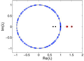
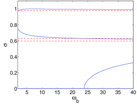
Figure 1: (Color online) Top panel: Floquet multiplier spectrum of the KMb for $L=5$ and $\omega_{\mathrm{b}}=15$; open (red) circles correspond to the unstable eigenvalues, theoretically predicted via the MI analysis. The unstable and neutral modes of the linearization are presented with (black) dots, while the neutrally stable ones on the unit circle are given by (blue) $\times$’s. Bottom panel: the dependence of the unstable eigenvalues $\sigma$ on the frequency $\omega_{b}$, for $L=5$. The solid line corresponds to the KMb numerically obtained multipliers, and dashed lines to the eigenvalues, once again theoretically predicted by the MI.

Apart from these modes, there are three pairs at $\lambda=1$: one of them corresponds to the translational mode, and another one to the phase mode (due to the conservation of the $L^{2}$ norm, i.e., the power in optics). The third pair stems, as is customary for breathers in Hamiltonian systems, from the time translational invariance. Finally, the remaining modes lie on the circle and correspond to background modes with a rather weak hybridization with the breather.

The top panel of Fig. 1 shows a summary of the above results, illustrating a typical example of the obtained FM spectrum and the instability eigenmodes, in the case $L=5$ and $\omega_{\mathrm{b}}=15$. This case leads to three double unstable multipliers for large $\omega_{\mathrm{b}}$ (as the domain expands, the number of unstable eigenmodes increases). One of these eigenvalues returns to the unit circle when $\omega_{\mathrm{b}}\approx 23.9$. The bottom panel depicts the dependence of the Floquet exponents $\sigma$ associated with the unstable modes, on the frequency of the breather. Notice that in the limit of large $\omega_{\mathrm{b}}$, the unstable Floquet exponents approach their asymptotic values predicted by the MI analysis above. On the other hand, for the FMs, $|\lambda|\rightarrow 1$, as $\omega_{b}\rightarrow\infty$. This limiting behavior of the FM modulus can be explained as follows: for $x\neq 0$, it follows from Eq. (2) that in the limit $\omega_{\mathrm{b}}\rightarrow\infty$, the solution $u_{\mbox{\tiny KM}}$ converges to $u_{\infty}=1$, of FM modulus $|\lambda|=1$. However, the convergence of $u_{\mbox{\tiny KM}}$ to the asymptotic state $u_{\infty}=1$ is not uniform. For $x=0$, in the limit $\omega_{b}\rightarrow\infty$, the solution $u_{\mbox{\tiny KM}}$ diverges. Hence, the KMb solution, being continuous itself as a function of the parameter $\omega_{\mathrm{b}}$, gives rise in the limit of large $\omega_{\mathrm{b}}$, via a slow, square-root rate divergence, to a “solitonic excitation” around $x=0$. This solitonic excitation is of finite localization width (for large, but finite $\omega_{\mathrm{b}}$) and of increasing (to infinity) amplitude. In accordance with Eq. (2), the limiting solitonic excitation on top of the unit background should consist of time-periodic peaks of vanishing period $T=2\pi/\omega_{\mathrm{b}}\rightarrow 0$, as $\omega_{\mathrm{b}}\rightarrow\infty$. This, however, does not affect the asymptotic behavior of the FM modulus $|\lambda|\rightarrow 1$.

Of particular importance is the opposite limit where the KMb approaches the PS. This is shown in the bottom panel of Fig. 1. It can be seen there that the lowest pair of the unstable modes returns to the unit circle, when $\omega_{\mathrm{b}}\approx 23.9$. However, there are also modes like the second (blue solid curve) mode in that panel whose growth rate monotonically increases as $\omega_{b}$ decreases. This is suggestive that the structure becomes progressively more unstable as the PS limit is approached –although it should be clarified that our computations are never able to precisely capture the limit; they can merely be characterized as strongly suggestive of the approach to it. There are also modes, like the one associated with the top-most (blue solid) curve in the panel, which may have a non-monotonic dependence on $\omega_{b}$, yet are still larger, for all values of the breather frequency, than their plane wave limit. Overall, this suggests that the presence of the KMb (and by virtue of the limiting process, the PS) enhances the instability of the background. Our results suggest that this conclusion extends towards the PS state which is approximated by the KMb as $\omega_{b}\rightarrow 0$.

To explore how our results depend on the size of the domain, we repeat the computationally expensive FM computation in the case of a domain twice as large, i.e., $L=10$ (and have confirmed the conclusions also by extending considerations even to $L=15$). In the case of $L=10$, we observe a similar scenario aside from the feature that there now exist six double unstable multipliers for high frequency. This is due to the fact that the increase of the domain size results in a “finer” quantization of wavenumbers which, in turn, means that more of the resulting wavenumbers find themselves in the unstable band of the MI spectrum.

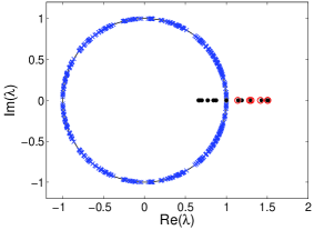
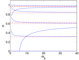
Figure 2: (Color online) Same as Fig. 1, but for $L=10$. It is clear that in this case the number of unstable modes is larger (in particularly, there are six, as can be counted in the bottom panel, shown by blue solid line, with their respective limiting values from the MI analysis given by red dashed line).

Figure 2 summarizes the aforementioned results for $L=10$, similarly to Fig. 1. A key feature becomes evident in both of the bottom panels of Figs. 1 and 2: there exist multiple unstable modes that have a stronger instability growth rate in the presence of the localized pattern (i.e., the KMb), rather than in its absence. This is true overall even though one pair of modes disappears into the unit circle for $\omega_{b}\approx 5.7$. Most of the rest of them (e.g., three clearly discernible examples in the bottom of Fig. 2) increase for decreasing $\omega_{b}$, while a couple may have non-monotonic or even decreasing dependence over $\omega_{b}$, although the overall growth rate is always higher in the presence of the KMb in comparison to the limit predicted by MI of the background state (dashed lines in the relevant panel). This is an interesting finding, indicating that the instability of the background is, in fact, overall enhanced by the presence of the KMb, and is strongly suggestive that this feature persists as the frequency is decreased towards the PS limit. On the other hand, that being said, it should be highlighted that there are no new unstable modes emerging solely due to the presence of the KMb: specifically, there is no point spectrum (no localized eigendirections) associated with the instability of the KMb.

In confirming these results for larger values of $L$, such as $L=15$, we have identified in the latter case 8 unstable pairs (say, for $\omega_{b}<2$). Among these, 5 pairs are found to show an increasing tendency, 2 to be decreasing, while 1 remains nearly invariant over our variation of $\omega_{b}$. Once again, no new unstable eigenmodes arise over the parametric scan –see Fig. 3.

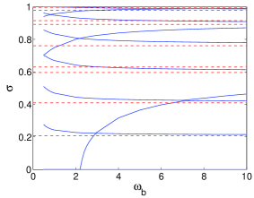
Figure 3: (Color online) Same as bottom panel of Fig. 2, but for $L=15$.

When $\omega_{b}$ is small, the Floquet exponents $\sigma$ approach finite values –see the bottom panel of Fig. 2– and we have checked that their unstable eigenmodes approach a limiting profile (data not shown). As computational power used for this problem is further enhanced, the Peregrine limit of $\omega_{b}\rightarrow 0$ of the KMb will become progressively more accessible. Nevertheless, it is important to appreciate that while going to lower frequencies, the periods of the breathers start growing to high values, and hence performance of the relevant computation becomes exceptionally demanding. This is not so much true at the level of the direct time integration, but most notably at that of the solution of the variational equations for the stability analysis which constitute a system of size $N^{2}\times N^{2}$ (where $N$ is the number of grid points used). While this is usually done for discrete breathers flach , typically the number of nodes can be restricted to $N\approx 100$ or so. However, in our case this being a continuum computation, the number of grid points to resolve the solution –even more notably so because of the space-time decay of a Peregrine soliton– is particularly large. More specifically, here we use $N=40L$ (typically $L=10$ is implemented), in accordance with the discretization parameter $\Delta x=0.05$ of the numerical integrator.

While we cannot fully extrapolate our results to the Peregrine limit, we do note that the trend of the instabilities observed is such that they only stem from the background and not from the localized core of the solution, a feature suggestive towards the relevant limit.

II.3 Direct Numerical Simulations

To elucidate the role of the above found instabilities on the dynamics, we have performed a series of direct numerical simulations for the NLS Eq. (1). The simulations concern the evolution of the KMb, being set as initial condition (at $t=0$, as $u_{\mbox{\tiny KM}}(x,t=0)$), perturbed along the direction of different unstable eigenmodes $\xi$; that is, the initial conditions used are of the form $u(x,t=0)=u_{\mbox{\tiny KM}}(x,0)+\delta\xi(x,0)$, with $\delta=10^{-3}$. Simulations have been performed for $L=10$ and $\omega_{b}=15$, although, for the sake of clarity, the figures only show the interval $[-5,5]$. Notice that for the value of $\omega_{\mathrm{b}}$ taken in the simulations, if $\delta=10^{-3}$ then $|u(\pm L,0)-1|\sim 10^{-5}$, so boundary effects are negligible.

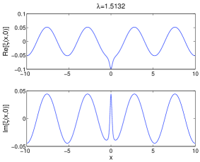
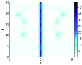
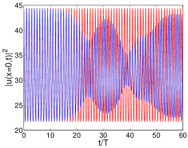
Figure 4: (Color online) KMb with $L=10$ and $\omega_{b}=15$. Top two panels: The spatial profiles, $\mathrm{Re}[\xi(x,0)]$ (first) and $\mathrm{Im}[\xi(x,0)]$ (second), of the unstable even eigenmode corresponding to $\lambda=1.5132$. Third panel: Contour plot of the evolution of the density $|u(x,t)|^{2}$, corresponding to a KMb initial condition (at $t=0$), perturbed along the direction of the unstable eigenmode portrayed in the top two panels. Bottom panel: comparison of the evolution of the center density (at $x=0$) of the breather [dark grey (blue) line], associated with the density evolution of the middle panel, against the respective evolution of the exact analytical KMb solution [light grey (red) line].

Before presenting our numerical findings, it is worth discussing at first the structure of the eigenmodes associated with the unstable and neutral eigenvalues. Generally, we have found that to each unstable eigenvalue corresponds a pair of degenerate, parity symmetric eigenmodes, with each one possessing even or odd symmetry. Both eigenmodes feature, asymptotically (for large $|x|$) an extended – periodic – structure, and are characterized by the presence of a localized peak (or dip) at the location of the KMb (at $x=0$); this peak is either even or odd for the respective even and odd eigenmode. Typical spatial profiles of the real and imaginary parts of even and odd eigenmodes, corresponding to $\lambda=1.5132$, are depicted in the two top panels of Figs. 4 and 5, respectively. For the limiting case of the neutral exponent with $\lambda=1$, the eigenmodes become localized in the vicinity of the KMb, tending asymptotically to zero.

We now proceed by investigating the effect of the above types of eigenmodes on the dynamics of the KMb. We observe that a perturbation along spatially even modes, such as the one pertinent to the unstable eigenvalue $\lambda=1.5132$ (cf. top two panels of Fig. 4), leads to the evolution depicted in the third and the bottom panels of Fig. 4, where a modulation of the breather, as well as a change of its frequency, are observed. Similar dynamics, although accompanied by a small-amplitude oscillation in the position of the breather, is also observed when the perturbation is along an odd mode eigendirection, such as the one corresponding to $\lambda=1.5132$ (cf. top two panels of Fig. 5). Notice that, in this case, the even KMb is perturbed by an odd eigenmode, which results in the emergence of this small-amplitude oscillation. The latter, is evident in the density evolution plot, shown in the third panel of Fig. 5.

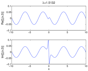
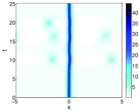
Figure 5: (Color online) Same as the three top panels of Fig. 4, but for the unstable odd eigenmode, corresponding to $\lambda=1.5132$. Here, it is observed that, due to the instability, the KMb performs a small-amplitude oscillation around its original location.

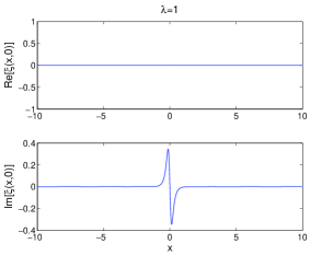
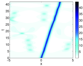
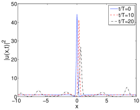
Figure 6: (Color online) Same as Fig. 5, but for the translational mode, corresponding to $\lambda=1$. The bottom panel shows the KMb profile at $t=0$ and when the breather has oscillated 10 and 20 periods. Notice the deformation of the background and the change of the maximum breather amplitude.

If the KMb is perturbed along the translational mode, it becomes mobile, as shown in Fig. 6. However, its evolution cannot be considered as following the typical traveling wave profile (4): the maximum amplitude of the breather changes in an oscillatory fashion when moving along the domain because of the interaction of the breather with the deformed background.

Notice that the dynamics of the KMb in all of the above cases takes place on top of the modulationally unstable background, as is evident in all space-time contour plots of Figs. 4, 5, and 6. Thus, while the KMb does not itself get destroyed, the underlying background gets distorted (as a result of the instability) during the evolution.

III Conclusions and Future Challenges

In the present work, we took a step towards exploring the spectral stability of rogue waves. In particular, we argued that given that these extreme events are limiting cases of other periodic (in the evolution variable) structures, it is possible to perform at first a Floquet stability analysis of the latter, and then try to a posteriori obtain suitable clues for the limiting case. This way, we focused on the spectral stability of the Kuznetsov-Ma breather (KMb), which –in the limit of infinite period– reduces to the Peregrine soliton (PS).

Our conclusions are two-fold. On the one hand, we discovered that the unstable modes commonly have a stronger instability growth rate in the presence of the KMb rather than in its absence, a conclusion which seems to be persisting as a trend as the frequency is decreasing towards the PS limit $\omega_{b}\approx 0$. In other words, this finding suggests that as the frequency decreases, the structure is more unstable than the background itself. This may be interpreted as stemming from the additional energy and the “seeding” of the instability of the background induced by the presence of the KMb. On the other hand, we observed the absence of any additional point spectrum (localized eigendirections), under the continuation of the KMb towards the Peregrine limit. This absence of point spectrum, intriguingly suggests the following: if some additional terms (linear/nonlinear) were incorporated in the original NLS model, such that a partial stabilization of the background was achieved, then the PS state would be more robust and, hence, more easily observable. Indeed, such a partial stabilization of the PS seems to to be the case in water waves, and similar experimentally tractable examples k2a -cap . Moreover, the perturbations that lead to dynamical instability, as shown in Figs.  4–6 may modify the frequency of the KMb or result in its mobility, but are not detrimental to the localized component of the structure per se. Based on the above arguments, we believe that, indeed, it is the above PS stabilization scenario which is relevant to the observability of the, otherwise unstable, rogue waves.

The present study, opens a number of paths for future exploration. Given the availability of the KMb in an explicit analytical form, while technically challenging, it is worthwhile to potentially ponder on the analytical tractability of the Floquet multiplier problem (especially in the light of the integrability of the 1D NLS model). Another interesting and relevant direction, is to explore the possibility of generalizing KMb solutions (and thereafter, their stability properties), to other models, such as extended NLS equations incorporating higher order effects devine ; themis . Finally, exploring whether Peregrine soliton solutions (and by extension, Kuznetsov-Ma breathers) may exist in higher-dimensional systems, is an intriguing topic in its own right, that merits further investigation. Some of these aspects are currently under consideration, and will be reported in future work.

Appendix A On the Floquet stability theory

In this Appendix, we provide brief information on the definition of the monodromy matrix $\mathcal{M}$ defined in Eq. (6), and its relevance to the stability problem of time-periodic solutions as the Kuznetsov-Ma breather (KMb) of Eq (1).

The linearized equation Eq. (5), can be written in the form of a system of first-order, linear evolution equations as follows:

$$\frac{d}{dt}V=\left[\begin{matrix}0&\mathcal{L}_{-}\\ -\mathcal{L}_{+}&0\end{matrix}\right]V=\mathcal{J}(t)V,$$ (9)

where $V=\left[\mathrm{Re}(\xi(x,t)),\mathrm{Im}(\xi(x,t))\right]^{T}$. The linear differential operators in the matrix $\mathcal{J}(t)$ of Eq. (9), are defined as $\mathcal{L}_{-}=-\frac{1}{2}\partial^{2}_{x}-2|u_{\mbox{\tiny KM}}|^{2}+1+u_{\mbox{\tiny KM}}^{2}$, and $\mathcal{L}_{+}=-\frac{1}{2}\partial^{2}_{x}-2|u_{\mbox{\tiny KM}}|^{2}+1-u_{\mbox{\tiny KM}}^{2}$. Due to the presence of the KMb solution $u_{\mbox{\tiny KM}}(x,t)$, the matrix $\mathcal{J}(t)$, is time-periodic with period $T=2\pi/\omega_{\mathrm{b}}$, i.e., $\mathcal{J}(t+T)=\mathcal{J}(t)$.

By numerical integration of (9) as described in Sec. II, we find its numerical (fundamental) solution $V(t)$, satisfying the relation

$$V(t+T)=V(t)V^{-1}(0)V(T).$$ (10)

Equivalently to Eq. (6), the monodromy matrix is defined by Eq. (10), as $\mathcal{M}=V^{-1}(0)V(T)$. On the other hand, Floquet’s theorem Pkh ; Li allows to reduce the fundamental solution of Eq. (9) in the form $V(t)=\Phi(t)\exp(tR)$, where $R$ is a constant matrix, and $\Phi(t)$ is periodic. Due to periodicity, it holds that

$$V(t+T) = \Phi(t+T)\exp[(t+T)R]$$ (11)

$$= V(t)\exp(TR).$$

Then, comparing Eq. (10) to Eq. (11), we may relate the monodromy matrix $\mathcal{M}$ with the matrix $R$, by the formula

$$\exp(TR)=V^{-1}(0)V(T)=\mathcal{M}.$$ (12)

It is evident from Eq. (12), that the eigenvalues of the monodromy matrix $\mathcal{M}$, the Floquet multipliers (FMs), determine the stability of the KMb (as they are associated through Eq. (12), to the eigenvalues of $R$, the corresponding Floquet exponents). The possibilities for FMs, and the induced instabilities, are as discussed in Sec. II.

Acknowledgments. P.G.K., D.J.F. and N.I.K. acknowledge that this work was made possible by NPRP grant # [8-764-160] from Qatar National Research Fund (a member of Qatar Foundation). The findings achieved herein are solely the responsibility of the authors. M.H. acknowledges the support of the ANR project BoND (ANR-13-BS01-0009-01) and the Labex ACTION program (ANR-11-LABX-01-01). J.C.-M. thanks financial support from MAT2016-79866-R project (AEI/FEDER, UE).

References

- (1) E. Pelinovsky and C. Kharif (eds.), Extreme Ocean Waves (Springer, NY, 2008).
- (2) C. Kharif, E. Pelinovsky, and A. Slunyaev, Rogue Waves in the Ocean (Springer, NY, 2009).
- (3) A. R. Osborne, Nonlinear Ocean Waves and the Inverse Scattering Transform (Academic Press, Amsterdam, 2010).
- (4) M. Onorato, S. Residori, F. Baronio, Rogue and Shock Waves in Nonlinear Dispersive Media, Springer-Verlag (Heidelberg, 2016).
- (5) A. Chabchoub, N. P. Hoffmann, and N. Akhmediev, Phys. Rev. Lett. 106, 204502 (2011).
- (6) A. Chabchoub, N. Hoffmann, M. Onorato, and N. Akhmediev, Phys. Rev. X 2, 011015 (2012).
- (7) A. Chabchoub and M. Fink, Phys. Rev. Lett. 112, 124101 (2014).
- (8) A. N. Ganshin, V. B. Efimov, G. V. Kolmakov, L. P. Mezhov-Deglin, and P. V. E. McClintock, Phys. Rev. Lett. 101, 065303 (2008).
- (9) D. R. Solli, C. Ropers, P. Koonath, and B. Jalali, Nature 450, 1054 (2007).
- (10) B. Kibler et al., Nature Phys. 6, 790 (2010).
- (11) B. Kibler et al., Sci. Rep. 2, 463 (2012).
- (12) J. M. Dudley, F. Dias, M. Erkintalo, and G. Genty, Nat. Photon. 8, 755 (2014).
- (13) B. Frisquet et al., Sci. Rep. 6, 20785 (2016).
- (14) C. Lecaplain, Ph. Grelu, J. M. Soto-Crespo, and N. Akhmediev, Phys. Rev. Lett. 108, 233901 (2012).
- (15) H. Bailung, S. K. Sharma, and Y. Nakamura, Phys. Rev. Lett. 107, 255005 (2011).
- (16) H. Xia, T. Maimbourg, H. Punzmann, and M. Shats, Phys. Rev. Lett. 109, 114502 (2012).
- (17) M. Shats, H. Punzmann, and H. Xia, Phys. Rev. Lett. 104, 104503 (2010).
- (18) D. H. Peregrine, J. Austral. Math. Soc. B 25, 16 (1983).
- (19) E. A. Kuznetsov, Sov. Phys.-Dokl. 22, 507 (1977).
- (20) Ya. C. Ma, Stud. Appl. Math. 60, 43 (1979).
- (21) N. N. Akhmediev, V. M. Eleonskii, and N. E. Kulagin, Theor. Math. Phys. 72, 809 (1987).
- (22) K. B. Dysthe and K. Trulsen, Phys. Scr. T82, 48 (1999).
- (23) Z. Yan, J. Phys. Conf. Ser. 400, 012084 (2012).
- (24) P. T. S. DeVore, D. R. Solli, D. Borlaug, C. Ropers, and B. Jalali, J. Opt. 15, 0640031 (2013).
- (25) M. Onorato, S. Residori, U. Bortolozzo, A. Montinad, and F. T. Arecchi, Phys. Rep. 528, 47 (2013).
- (26) N. Akhmediev, J.M. Soto-Crespo, A. Ankiewicz, Phys. Lett. A 373, 2137 (2009).
- (27) A. Ankiewicz, N. Devine, N. Akhmediev, Phys. Lett. A 373, 3997 (2009).
- (28) A. Calini and C. M. Schober, pp. 31–51 in Ref. k2a .
- (29) L. Gagnon, J. Opt. Soc. Am. B 10, 469 (1993).
- (30) J. Garnier and K. Kalimeris, J. Phys. A: Math. Theor. 45, 035202 (2012).
- (31) C. Klein and M. Haragus, arXiv:1507.0676, Ann. Math. Sci. Appl., to appear.
- (32) A. Calini and C. M. Schober, Nat. Hazards Earth Syst. Sci. 14, 1431 (2014).
- (33) A. Calini and C. M. Schober, Nonlinearity 25, R99 (2012).
- (34) K. Dysthe, Proc. R. Soc. Lond. A 369, 105 (1979).
- (35) R. A. Van Gorder, J. Phys. Soc. Jpn. 83, 054005 (2014).
- (36) U. Al Khawaja, H. Bahlouli, M. Asad-uz-zaman, S.M. Al-Marzoug, Commun. Nonlinear Sci. Numer. Simulat. 19, 2706 (2014).
- (37) U. Al Khawaja, S.M. Al-Marzoug, H. Bahlouli, M. Asad-uz-zaman, Commun. Nonlinear Sci. Numer. Simulat. 32, 1 (2016).
- (38) K. McQuighan and C.E. Wayne, arXiv:1601.05363.
- (39) See, e.g., https://www.youtube.com/watch?v=LHqYqiYBSE0.
- (40) C. Sulem and P.L. Sulem, The Nonlinear Schrödinger Equation, Springer-Verlag (New York, 1999).
- (41) M.J. Ablowitz, B. Prinari and A.D. Trubatch, Discrete and Continuous Nonlinear Schrödinger Systems, Cambridge University Press (Cambridge, 2004).
- (42) V.E. Zakharov, L.A. Ostrovsky, Phys. D 238, 540 (2009).
- (43) S. Flach and A. V. Gorbach, Phys. Rep. 467, 1 (2008).
- (44) A-K Kassam and LN Trefethen. SIAM J. Sci. Comput. 26, 1214 (2005).
- (45) S.M. Cox, P.C. Matthews, J. Comput. Phys. 176 430 (2002).
- (46) A.-K. Kassam, Solving reaction-diffusion equations 10 times faster, preprint (2003).
- (47) W. Cousins and T.P. Sapsis Phys. Rev. E 91, 063204 (2015).
- (48) P.A. Kuchment, Floquet Theory for Partial Differential Equations (Birkhäuser, Basel, 1993).
- (49) Y. Li and D. W. McLaughlin, Commun. Math. Phys. 162, 175 (1994).