On calculation of RKKY range function in one dimension

Abstract

The effect of strong singularity in the calculation of range function for the RKKY interaction in 1D electron gas is discussed. The method of handling this singularity is presented. A possible way of avoiding the singularity in the Ruderman-Kittel perturbation theory in 1D is described.

I Introduction

Some years after the discovery of Ruderman-Kittel-Kasuya-Yosida (RKKY) interaction between localized magnetic moments in three dimensions Ruderman1954 , Kittel considered an extension of this interaction to lower dimensional system Kittel1968 . In the late 1980’s and beginning of the 1990’s the RKKY interaction was recognized as one of the mechanisms of coupling between magnetic layers in metallic superlattices Bruno1992 , and the energy of RKKY interaction in quasi 1D systems was determined experimentally by Parkin and Mauri Parkin1991 . A review of these efforts is summarized in Ref. Yafet1994 . Later, the RKKY interaction in 1D or quasi-1D systems was investigated in many other works, see e.g. Imamura2004 , and this subject is of actuality until present days, see e.g. Nejati2017 . For this reason, all subtleties of this problem should be clarified.

In his work, Kittel calculated the energy of RKKY interaction in one dimension between two localized magnetic moments embedded in a free electron gas Kittel1968 . He calculated first the magnetic susceptibility $\chi(q)$ of the electron gas in the presence of magnetic moments and then the range function was obtained as the Fourier transform of $\chi(q)$. In the appearing integral Kittel changed the order of integration which lead to erroneous results predicting a finite interaction energy at infinite distance between localized moments. This error was corrected in the Erratum to Ref. Kittel1968 , and the correct result was obtained with a reverse order of integration. Some time later Yafet Yafet1987 showed that the problem reported by Kittel is caused by the presence of a strong singularity of the double integral at $k=q=0$ and, because of the singularity, it is not allowed to change the order of integration over $k$ and $q$ variables. To show this, Yafet calculated twice the range function taking different orders of integrations and obtained different results. Then he determined the correct order of integrations. Further subtleties of this problem were discussed by Guliani et al. Giuliani2005 . Litvinov and Dugaev Litvinov1998 showed that an application of Green’s function formalism allows one to avoid singularities at $k=q=0$.

There exists an alternative method to calculate the RKKY interaction proposed in the original approach of Ruderman and Kittel (RK) to the 3D case Ruderman1954 . This method is based on a direct calculation of the second order correction to the energy of free electron gas in the presence of two localized magnetic moments. In 3D one obtains a double integral over $|k^{\prime}|>k_{F}$ and $|k|\leq k_{F}$ domain, which does not contain the strong singularity. This integral is then replaced by a difference of two integrals. Applying this procedure to 1D gas one finds that, surprisingly, each of the two integrals contains a strong singularity at $k=k^{\prime}=0$. This singularity does not exists in 2D or 3D cases. But in the 1D case there appears a singularity which is analogous to that appearing in the calculation of the range function in one dimension with the use of susceptibility $\chi(q)$ discussed by Yafet Yafet1987 .

In the present note we analyze the effect of strong singularity at $k=k^{\prime}=0$ on the range function of the RKKY interaction in 1D calculated with the use of RK approach. Our results extend previous analyzes of singularities appearing in the calculations of the range function with use of susceptibility $\chi(q)$ in 1D, as described in Refs Kittel1968 ; Yafet1987 ; Giuliani2005 . Then we show the effect of the order of integration over the singular part of the integral in the 1D case and determine the correct order of integration. Finally we propose another way to calculate the range function using a domain that is free of strong singularities.

II Theory

Let us consider a one-dimensional free electron gas. Let the two spins $\hat{\bm{S}}_{i}$ be located at ${\bm{R}}_{i}$, where $i=1,2$. A coupling between the conduction electrons and the localized spins is assumed in the form of s-d interaction

$$\hat{H}_{sd}=\frac{J_{sd}}{N_{1D}}\sum_{i=1,2}\delta({\bm{R}}-{\bm{R}}_{i})\hat{\bm{S}}_{i}\hat{\bm{\sigma}},$$ (1)

where $\hat{\bm{\sigma}}$ is electron spin operator, $J_{sd}$ is the energy of s-d coupling, and $N_{1D}$ is the one-dimensional density of magnetic atoms. Note that $J_{sd}/N_{1D}$ has the dimensionality of [energy] $\times$ [length]. Following Ruderman and Kittel, the second order correction to the energy of electron gas perturbed by localized spins is Ruderman1954

$$\Delta E^{(2)}=\frac{J_{sd}^{2}}{(2\pi)^{2}N_{1D}^{2}}\frac{2m^{*}}{\hbar^{2}}\hat{\bm{S}}_{i}\hat{\bm{S}}_{j}F_{1D}(r)$$ (2)

where

$$F_{1D}(r)=\int_{-k_{F}}^{k_{F}}dk\left[\left(\int_{-\infty}^{-k_{F}}+\int_{k_{F}}^{\infty}\right)\frac{\cos(kr)\cos(k^{\prime}r)}{k^{\prime 2}-k^{2}}dk^{\prime}\right],\ \$$ (3)

in which $m^{*}$ is the electron effective mass, $k_{F}$ is the Fermi vector, $r=R_{i}-R_{j}$, and $F_{1D}(r)$ is the so-called range function. The order of integration in Eq. (3) follows from the method of calculation of $\Delta E^{(2)}$: first one selects the wave vector $k$, calculates the second order correction $\Delta E^{(2)}_{k}$ to the electron’s energy $E_{k}$ [square bracket in Eq. (3)], and then sums $\Delta E^{(2)}_{k}$ over $k$ within the 1D Fermi sphere. Considering Eq. (3) one concludes that, since the $k$ vectors are inside the 1D Fermi sphere and the $k^{\prime}$ vectors are outside the sphere, the denominators in Eq. (3) are always nonzero and no singularity occurs.

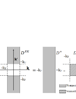
Figure 1: Schematic visualization of integration domain defined in (4)–(6). Left side of equation: domain of integration in Eq. (3) (grey), right side: two domains of integration proposed in Ref. Ruderman1954 , gray and dotted. Grey areas give nonzero contribution to the range function while integral over dotted areas vanishes due to symmetry.

The difficulty in Eq. (3) is that the integral over $dk^{\prime}$ can not be calculated analytically. To overcome this problem RK Ruderman1954 proposed to replace the integral in Eq. (3) over the domain

$${\cal D}^{RK}:(k,k^{\prime})\in[-k_{F},k_{F}]\times\mathbb{R}\setminus[-k_{F},k_{F}],$$ (4)

by the difference of two integrals over domains

$${\cal D}^{a} : (k,k^{\prime})\in[-k_{F},k_{F}]\times\mathbb{R},$$ (5)

$${\cal D}^{b} : (k,k^{\prime})\in[-k_{F},k_{F}]\times[-k_{F},k_{F}],$$ (6)

see Figure 1. In the above expressions we used the notation of the set theory. As an example, if $k$ is a member of set ${\cal A}$, the notation $k\in{\cal A}$ is used. Similarly, $\times$ denotes the cartesian product of two sets, ${\cal A}\setminus{\cal B}$ denotes difference between the two sets, and ${\cal A}\cup{\cal B}$ means the union of the two sets. For more detailed description of set notion see Ref. WikiSets .

From (4)–(6) we have

$$F_{1D}(r)=\int{\cal D}^{RK}=\int{\cal D}^{a}-\int{\cal D}^{b},$$ (7)

in which we use the notation

$$\int{\cal D}^{a}=\iint_{(k,k^{\prime})\in{\cal D}^{a}}\left(\frac{\cos(kr)\cos(k^{\prime}r)}{k^{\prime 2}-k^{2}}dk^{\prime}\right)dk,$$ (8)

and similarly for ${\cal D}^{b}$ and ${\cal D}^{RK}$. This method works correctly for 3D. However, doing so for 1D requires caution due to the presence of strong singularity at $k=k^{\prime}=0$ in Eq. (8) for the domains ${\cal D}^{a}$ and ${\cal D}^{b}$. We show below that this method may not be directly applied to the 1D case since the singularity at $k=k^{\prime}=0$ gives a nonzero contribution to the integrals.

Consider first $\int{\cal D}^{a}$, as given in Eqs. (5) and (8). The integral over $k^{\prime}$ is obtained with the use of formula 3.723.9 in GradshteinBook

$$\int_{-\infty}^{\infty}\frac{\cos(rk^{\prime})}{k^{2}-k^{\prime 2}}dk^{\prime}=\frac{\pi}{k}\sin(rk),$$ (9)

which is valid for $|r|,|k|>0$. Then

$$\int{\cal D}^{a}=-\pi\int_{-k_{F}}^{k_{F}}\frac{\cos(kr)\sin(kr)}{k}dk=-\pi{\rm Si}(2k_{F}r),$$ (10)

where ${\rm Si}(x)=\int_{0}^{x}(\sin(t)/t)dt$ is the sine-integral in the standard notation, see GradshteinBook .

The subtle point in the derivation of Eq. (10) is that the integral on the left hand side of Eq. (9) does not exist at $k=0$, since for $k=0$ and $|k^{\prime}|\rightarrow 0$ the integrand diverges as $1/k^{{}^{\prime}2}$. Therefore Eq. (9) in valid for all ${\cal D}^{a}$ except in the small domain

$${\cal D}^{\epsilon}:(k,k^{\prime})\in[-\epsilon,\epsilon]\times[-\epsilon,\epsilon],$$ (11)

with $\epsilon\rightarrow 0$, for which the identity (9) can not be used. To overcome this problem we isolate the domain ${\cal D}^{\epsilon}$ out of the integration domain: $\int{\cal D}^{a}=\int{\cal D}^{a\epsilon}+\int{\cal D}^{\epsilon}$, in which: ${\cal D}^{a\epsilon}={\cal D}^{a}\setminus{\cal D}^{\epsilon}$. The contribution to the range function coming from ${\cal D}^{\epsilon}$ has to be calculated separately.

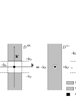
Figure 2: Schematic visualization of difference of the two domains shown in Eq. (12). Grey and dotted areas have the same meaning as in Figure 1. Black squares: strong singularity at $k=k^{\prime}=0$. Note that the two domains on the rhs still do not include strong singularity.

Turning to $\int{\cal D}^{b}$ we note that there is a similar problem with the singularity at $k=k^{\prime}=0$, so that we again isolate ${\cal D}^{\epsilon}$ out of the integration domain: $\int{\cal D}^{b}=\int{\cal D}^{b\epsilon}+\int{\cal D}^{\epsilon}$ in which: ${\cal D}^{b\epsilon}={\cal D}^{b}\setminus{\cal D}^{\epsilon}$. Let us assume that the integral ${\cal D}^{\epsilon}$ is finite, which is crucial for the calculations. Then from Eq. (7) we have (see Figure 2)

$$F_{1D}(r) = \int\left({\cal D}^{a\epsilon}\cup{\cal D}^{\epsilon}\right)-\int\left({\cal D}^{b\epsilon}\cup{\cal D}^{\epsilon}\right)$$ (12)

$$= \int{\cal D}^{a\epsilon}-\int{\cal D}^{b\epsilon}.$$

Thus, if the integral $\int{\cal D}^{\epsilon}$ is finite, the contribution arising from the two integrals $\int{\cal D}^{\epsilon}$ in Eq. (12) cancels out. However, in order to apply Eq. (10) one has to calculate the integral over the domain ${\cal D}^{a}$ instead of ${\cal D}^{a\epsilon}$. Assuming that $\int{\cal D}^{\epsilon}$ is finite we can rewrite Eq. (12) as

$$F_{1D}(r)=\int{\cal D}^{a}-\int{\cal D}^{b\epsilon}-\int{\cal D}^{\epsilon},$$ (13)

in which $\int{\cal D}^{a}$ is given in Eq. (10), see Figure 3.

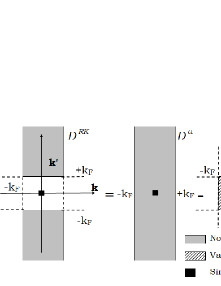
Figure 3: Schematic visualization of difference of the three domains shown in (13). Grey and dotted areas have the same meaning as in Figure 1. Note that on the rhs the strong singularity (black square) is added to ${\cal D}^{a}$ and explicitly subtracted. This is the main difference between the 3D case in which the strong singularity does not exist, see text.

This is the final result of our manipulations. Since there is no strong singularity in ${\cal D}^{b\epsilon}$, we may apply the method proposed in Ref. Ruderman1954 and show that $\int{\cal D}^{b\epsilon}=0$, see Appendix A. Comparing Eq. (13) with Eq. (4) we note the additional contribution in 1D from $\int{\cal D}^{\epsilon}$ to the range function, which does not exist in 3D, see Figures 1 and 3.

To calculate $\int{\cal D}^{\epsilon}$ we use a similar approach to that applied by Yafet Yafet1987 . We first approximate in Eq. (8): $\cos(kr)\simeq 1$ and $\cos(k^{\prime}r)\simeq 1$, which is valid for sufficiently small $|k|$ and $|k^{\prime}|$. Then we have

$$\int{\cal D}^{\epsilon}=\int_{-\epsilon}^{\epsilon}dk\int_{-\epsilon}^{\epsilon}\frac{dk^{\prime}}{k^{\prime 2}-k^{2}}.$$ (14)

Using the identity: $1/(k^{\prime 2}-k^{2})=(1/2k)[1/(k^{\prime}-k)-1/(k^{\prime}+k)]$ and integrating in Eq. (14) over $k^{\prime}$ we find that $\int{\cal D}^{\epsilon}$ is nonzero

$$\int{\cal D}^{\epsilon}=\int_{-\epsilon}^{\epsilon}\left(\frac{\ln|\epsilon-k|}{k}-\frac{\ln|\epsilon+k|}{k}\right)dk=$$

$$\int_{-1}^{1}\left(\frac{\ln|1-u|}{u}-\frac{\ln|1+u|}{u}\right)du=$$

$$=-2{\rm Li}_{2}(1)+2{\rm Li}_{2}(-1)=-\frac{\pi^{2}}{2}.$$ (15)

This is the peculiarity of 1D case, which does not appear in 2D and 3D, see Appendix B. In the above equation: ${\rm Li}_{2}(x)=-\int_{0}^{x}du\ln|1-u|/u$ is the dilogarithm function, see GradshteinBook ; Mitchell1949 ; LewinBook , and we have used: ${\rm Li}_{2}(1)=\pi^{2}/6$ and: ${\rm Li}_{2}(-1)=-\pi^{2}/12$, see GradshteinBook . Collecting the results from Eqs. (10), (13) and (II) we have

$$F_{1D}(r)=\pi\left[\frac{\pi}{2}-{\rm Si}(2k_{F}r)\right],$$ (16)

which agrees with the results reported in the literature Yafet1987 ; Giuliani2005 ; Litvinov1998 . The range function in Eq. (16) oscillates with the period: $T_{r}=\pi/k_{F}$ and decays to zero at large distances between spins. Note that neglecting the contribution from $\int{\cal D}^{\epsilon}$ one erroneously obtains: $F_{1D}(r)=\int{\cal D}^{a}\propto{\rm Si}(2k_{F}r)$, see Kittel1968 , which for large $r$ tends to a finite value.

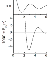
Figure 4: Upper panel: The range function $F_{1D}(r)$, as given in Eq. (16). Lower panel: The range function $F_{3D}(r)$, see text. Please note the difference in scales between two panels

In order to illustrate $F_{1D}(r)$ we plot this function in Figure 4a, and compare it with the widely-known range function in 3D: $F_{3D}(z)=[\sin(z)-z\cos(z)]/z^{4}$ with $z=2k_{F}r$, see Figure 4b. As seen in the Figures, both functions have the same oscillation period, and both vanish at $k_{F}r\rightarrow\infty$, but the function $F_{1D}(r)$ decays as $r^{-1}$, i.e. much slower than $F_{3D}(r)$.

In the calculation of $\int{\cal D}^{\epsilon}$ it is not allowed to change the order of integration over $k$ and $k^{\prime}$ variables. To show this we calculate an integral $\int{\cal D}^{\epsilon}_{R}$ in analogy to that in Eq. (14), but with the reversed order of integration over $k$ and $k^{\prime}$. Using the identity: $1/(k^{\prime 2}-k^{2})=(1/2k^{\prime})[1/(k^{\prime}-k)+1/(k^{\prime}+k)]$ one obtains

$$\int{\cal D}^{\epsilon}_{R}=\int_{-\epsilon}^{\epsilon}\left(\frac{-\ln|\epsilon-k^{\prime}|}{k^{\prime}}+\frac{\ln|\epsilon+k^{\prime}|}{k^{\prime}}\right)dk^{\prime}=$$

$$=2{\rm Li}_{2}(1)-2{\rm Li}_{2}(-1)=+\frac{\pi^{2}}{2}.$$ (17)

Thus $\int{\cal D}^{\epsilon}_{R}\neq\int{\cal D}^{\epsilon}$, so the change in the order of integration over $k$ and $k^{\prime}$ is not allowed.

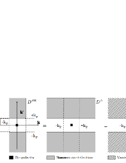
Figure 5: Schematic visualization of integration domain defined in (18). Grey and dotted areas have the same meaning as in Figure 1. Note that on the rhs the domains of integration do not include the strong singularity, so one can safely change the order of integration over $k$ and $k^{\prime}$, see Eq. (21).

In 1D one can avoid the problem with the strong singularity at $k=k^{\prime}=0$ by replacing the domain ${\cal D}^{RK}$ in Eq. (4) by another one, still free of the strong singularity. For example, one can choose domain ${\cal D}^{f}$ defined as

$${\cal D}^{f} : {\cal D}^{A}\setminus\left({\cal D}^{++}\cup{\cal D}^{+-}\cup{\cal D}^{-+}\cup{\cal D}\right),$$ (18)

$${\cal D}^{A} : (k,k^{\prime})\in\mathbb{R}\times\left([k_{F},\infty)\cup[k_{F},\infty)\right),$$ (19)

$${\cal D}^{++} : (k,k^{\prime})\in[k_{F},\infty)\times[k_{F},\infty).$$ (20)

The domain ${\cal D}^{++}$ describes the right upper corner of the $k\times k^{\prime}$ plane, while domains ${\cal D}^{+-}$, ${\cal D}^{-+}$ and ${\cal D}^{--}$ describe its three remaining corners, see Figure 5. Since there are no strong singularities in any of the above domains, in each domain of (18)–(20) it is allowed to change the order of integration over $k$ and $k^{\prime}$ vectors. Using similar arguments to those in Appendix A we obtain: $\int({\cal D}^{++}\cup{\cal D}^{+-}\cup{\cal D}^{-+}\cup{\cal D}^{--})=0$, and then: $\int{\cal D}^{f}=\int{\cal D}^{A}$. Changing the order of integration in ${\cal D}^{A}$ and calculating first the integral over $k$ with use of Eq. (9) we find

$$F_{1D}(r)=\pi\!\int_{k_{F}}^{\infty}\!\frac{\sin(2k^{\prime}r)}{k^{\prime}}dk^{\prime}=\pi\left(\frac{\pi}{2}-{\rm Si}(2k_{F}r)\right),$$ (21)

in which $\lim_{x\rightarrow\infty}{\rm Si}(x)=\pi/2$, see GradshteinBook . This agrees with Eq. (16). Note that for ${\cal D}^{A}$ there is always: $|k^{\prime}|>k_{F}>0$ and the integrand over $k$ on the left hand side of Eq. (9) exists for all $k^{\prime}$ in the domain ${\cal D}^{A}$.

Comparing Figures 1, 2 and 3 with Figure 5 we note that the transformed domains on the right-hand sides of Figures 1, 2 and 3 are ’vertical’ in the $k-k^{\prime}$ plane, while the corresponding domain in Figure 5 is ’horizontal’ one. This seemingly minor change allows one to avoid any singularity appearing for small values of both $k$ and $k^{\prime}$ vectors. Turning to the initial domain of integration, as indicated on the left-hand side of Figure 5, we see that this domain is limited to $|k|\leq k_{F}$ and $|k^{\prime}|>k_{F}$, i.e. it does not include strong singularity at $k=k^{\prime}=0$. For sufficiently large $k_{F}$ the existence or no-existence of the singularity at the origin should not alter the integration over the RK domain. Thus the singularity is only an artefact appearing in 1D case without an impact on the range function $F_{1D}(r)$. But in the arrangement proposed by RK, as seen in Figures 1, 2 and 3, one replaces the singularity-free domain by a combination of domains including the singularity, which requires strict mathematical rigor in handling the problem. In contrast, in the arrangement shown in Figure 5 one transforms the singularity-free domain by a combination of five singularity-free domains, and the correct results are obtained in a straightforward way, see Eq. (21).

III Discussion and summary

The problem arising in the calculation of interaction energy with the use of the perturbation expansion, as expressed in Eqs. (2) and (3), is to justify a truncation of the expansion to the second order terms. In general, the perturbation series is convergent if there exists a ’small parameter’ $\alpha\simeq V(r)/(E_{k}-E_{k^{\prime}})\ll 1$. Turning to Eq. (3) we may suspect that, possibly, the perturbation expansion may not converge for states $k^{\prime}$ lying close to the Fermi sphere $k_{F}$ since in this case $E_{k}^{\prime}\simeq E_{k}$, and the denominator in Eq. (3) is small.

To analyze this effect quantitatively we calculate a contribution of $\delta E^{(2)}$ to the interaction energy $\Delta E^{(2)}$ arising from states $k^{\prime}$ belonging to small slices close to the Fermi level: $k^{\prime}\in(k_{F},k_{F}+\delta k]\cup[-k_{F}-\delta k,-k_{F})$, with $\delta k_{F}\ll k_{F}$. We define the integration domain

$${\cal D}^{\delta k^{\prime}}:(k,k^{\prime})\in[-k_{F},k_{F}]\times\left((k_{F},k_{F}+\delta k]\cup[-k_{F}-\delta k,-k_{F})\right),$$ (22)

and calculate the range function $F_{1D}(r)$ on this domain. The calculations are analogous to those in Eqs. (18)–(21), but with the integration over $k^{\prime}$ limited to $\pm(k_{F}+\delta k)$ instead of $\pm\infty$, respectively. Then we obtain from Eq. (21)

$$\delta E^{(2)}\propto\pi\!\int_{k_{F}}^{k_{F}+\delta k}\!\frac{\sin(2k^{\prime}r)}{k^{\prime}}dk^{\prime}\simeq\pi\frac{\sin(2k_{F}r)}{k_{F}}\delta k.$$ (23)

The the Fermi vector $k_{F}=2\pi/\lambda_{F}$ entering into the RKKY range function in Eqs. (21) and (23) was first measured directly by Parkin and Mauri in Ni₈₀Co₂₀/Ru superlattices Parkin1991 . The authors reported $\lambda_{F}=11.5$ Å, which gives $k_{F}=0.55$Å^-1. Other values found in the literature are on the order of $k_{F}\simeq 0.5$ Å^-1–$1.2$ Å^-1, see Ref. Yafet1994 and references therein. For such values of $k_{F}$ the energy $\delta E^{(2)}$ in Eq. (23) does not diverge and the second order perturbation approach is justified.

A contribution of third-order terms to RKKY in 3D was calculated in Ref. Vertogen1966 and it turned out that these terms are divergent at the limit $k^{\prime}\rightarrow\infty$ of integration over excited states $k^{\prime}$. This may possibly occur also in 1D case. However, as shown in Bowen1968 , the motion of atoms due to phonons removes the divergence in the third-order energy. On the other hand, an approximation of the realistic energy bands by the parabolic dispersion is valid only up to a certain value of $k_{max}$, which may not exceed edges of the Brillouin zone: $k_{BZ}\simeq 2\pi/a_{latt}\simeq 2.5$ Å^-1 for typical values of lattice constants $a_{latt}$. Therefore, the divergence appearing for $k^{\prime}\rightarrow\infty$ is not physical. Introducing a reasonable cut-off in the $k^{\prime}$ integration, or taking more realistic (e.g. tight-binding like) energy dispersion, one obtains finite results for all dimensions. Thus introducing the cut-off in the calculation of third-order terms, a strong singularity at $k=k^{\prime}=0$ may also be removed by methods discussed in our paper. The resulting interaction would include higher powers of $\hat{\bm{S}}_{1}\hat{\bm{S}}_{2}$ operators, see e.g. Doman1969 .

In summary, we analyzed the effect of strong singularity in the calculation of range function for RKKY interaction in one dimension using the Ruderman-Kittel method. This approach is complementary to the more frequently used method based on the susceptibility of the free electron gas. It is pointed out that, in the RK method applied to the one-dimensional gas, the initial singularity-free integral is replaced by two integrals, each of them including strong singularity at $k=k^{\prime}=0$. The way of isolating the singular parts of the two integrals is derived and the method of handling the singularity is described. It is shown that the integral over the singularity depends on the order of integration over $k$ and $k^{\prime}$ vectors and the correct order of integration is determined. The reason for disappearance of the singularity in higher dimensions is explained. Importantly, a possible way of avoiding the singularity in one dimension is proposed, see Figure 5. Our analysis should help to avoid similar difficulties which may occur in other low-dimensional systems.

Appendix A

We show that $\int{\cal D}^{b\epsilon}=0$, see Eq. (II). Let $J^{b\epsilon}_{k^{\prime}k}=\int{\cal D}^{b\epsilon}$, where the lower indices define the order of calculation in the integrals. By changing variables: $(k,k^{\prime})\rightarrow(k^{\prime},k)$ we find: $J^{b\epsilon}_{k^{\prime}k}=-J^{b\epsilon}_{kk^{\prime}}$, because of the change of signs in the denominators, see Eq. (II). Since there is no strong singularity in ${\cal D}^{b\epsilon}$, the integral $\int{\cal D}^{b\epsilon}$ does not depend on the order of integration over $k$ and $k^{\prime}$ variables. Then we have: $J^{b\epsilon}_{k^{\prime}k}=J^{b\epsilon}_{kk^{\prime}}$ which gives the desired result: $J^{b\epsilon}_{kk^{\prime}}=-J^{b\epsilon}_{kk^{\prime}}\Leftrightarrow\int{\cal D}^{b\epsilon}=0$. This also occurs for integrals over any domain ${\cal D}^{s}$ symmetric within $k$ and $k^{\prime}$ variables. Using the same arguments one may show that $\int{\cal D}^{b\epsilon}=0$ and $\int{\cal D}^{++}+{\cal D}^{+-}+{\cal D}^{-+}+{\cal D}^{--}=0$, see Eq. (20) and Figure 5.

Appendix B

The problem with the integration over ${\cal D}^{\epsilon}$ does not exist in two and three dimensions since in these cases there is no strong singularity at $k=k^{\prime}=0$. In this Appendix we quote for completeness the corresponding calculations. In 3D, after integration over angular variables, one obtains for the range function (see Eq. (6) in Ruderman1954 ),

$$F_{3D}(r)=\int_{-k_{F}}^{k_{F}}\int_{-k_{F}}^{k_{F}}\frac{e^{ir(k+k^{\prime})}kk^{\prime}}{k^{{}^{\prime}2}-k^{2}}dk^{\prime}dk,$$ (24)

which has no contribution from the singularity at $k=k^{\prime}=0$ because of the $kk^{\prime}$ factor in the integrand. To show this we calculate the integral in Eq. (24) over domain ${\cal D}^{\epsilon}$, see Eq. (14). For small $|k|$ and $|k^{\prime}|$ there is: $e^{ir(k+k^{\prime})}\rightarrow 1$ and, instead of Eqs. (14)–(II), we have

$$\int{\cal D}^{\epsilon}_{3D}=\int_{-\epsilon}^{\epsilon}\int_{-\epsilon}^{\epsilon}\frac{kk^{\prime}}{k^{{}^{\prime}2}-k^{2}}dk^{\prime}dk=0,$$ (25)

Thus, there indeed is no contribution from the singularity at $k=k^{\prime}=0$. The same result is obtained for the reversed order of calculation in the integrals in Eq. (25), so that $\int{\cal D}^{\epsilon}_{3D}$ does not depend on the order of integration over $k$ and $k^{\prime}$. Similar arguments can be used for calculating the range function in 2D, in which also the volume element $kk^{\prime}\ dkdk^{\prime}$ appears.

References

- (1) M. A. Ruderman and C. Kittel, Phys. Rev. 96, 99 (1954).
- (2) C. Kittel, in Solid State Physics, edited by F. Seitz, D. Turnbull, and H. Ehrenreich (Academic, New York, 1968), Vol. 22, p. 1.
- (3) P. Bruno and C. Chappert, Phys. Rev. B 46, 261 (1992).
- (4) S. S. P. Parkin and D. Mauri, Phys. Rev. B 44, 7131 (1991).
- (5) Y. Yafet, in Magnetic Multilayers, edited by L. H. Bennett and R. E. Watson (World Scientific, Singapore, 1994), p.19
- (6) H. Imamura, P. Bruno, and Y. Utsumi, Phys. Rev. B 69, 121303(R) (2004).
- (7) A. Nejati and J. Kroha, J. Phys.: Conf. Series, 807, 082004 (2017).
- (8) Y. Yafet, Phys. Rev. B 36, 3948 (1987).
- (9) G. F. Giuliani, G. Vignale, and T. Datta, Phys. Rev. B 72, 033411 (2005).
- (10) V. I. Litvinov and V. K. Dugaev, Phys. Rev. B 58, 3584 (1998).
- (11) Set theory, URL https://en.wikipedia.org/wiki/Set_theory, (2017).
- (12) I. S. Gradshtein and I. M. Ryzhik in Table of Integrals, Series, and Products, 7th ed., edited by A. Jeffrey and D. Zwillinger (Academic Press, New York, 2007).
- (13) K. Mitchell, Philos. Mag. 40, 351 (1949).
- (14) L. Lewin Dilogarithms and associated functions (Macdonald, London, 1958).
- (15) G. Vertogen and W. J. Gaspers, Phys. Rev. Lett. 16, 904 (1966).
- (16) S. P. Bowen, Phys. Rev. Lett. 20, 726 (1968).
- (17) B. G. S. Doman, Phys. Lett. A 29, 349 (1969).