Greedy Structure Learning of Hierarchical Compositional Models
Abstract
In this work, we consider the problem of learning a hierarchical generative model of an object from a set of images which show examples of the object in the presence of variable background clutter. Existing approaches to this problem are limited by making strong a-priori assumptions about the object’s geometric structure and require segmented training data for learning. In this paper, we propose a novel framework for learning hierarchical compositional models (HCMs) which do not suffer from the mentioned limitations. We present a generalized formulation of HCMs and describe a greedy structure learning framework that consists of two phases: Bottom-up part learning and top-down model composition. Our framework integrates the foreground-background segmentation problem into the structure learning task via a background model. As a result, we can jointly optimize for the number of layers in the hierarchy, the number of parts per layer and a foreground-background segmentation based on class labels only. We show that the learned HCMs are semantically meaningful and achieve competitive results when compared to other generative object models at object classification on a standard transfer learning dataset.
1 Introduction
Object analysis in natural images requires generalization from limited observations to a potentially infinite amount of image patterns that are generated by variations of an objects geometry, appearance and background clutter. Generative object modeling [14, 40, 2] is a highly promising approach to object analysis as it naturally integrates different analysis tasks, such as detection, segmentation and classification, into a joint reasoning process. However, so far the learning of generative object models requires detailed human supervision during training, while posterior inference at test time is slow. Hierarchical compositional generative models [17, 9, 39] proposed to resolve these issues by enforcing a more efficient representation that allows for fast inference, feature sharing and contextual reasoning. Such hierarchical compositional models (HCMs) demonstrated impressive generalization capabilities for a diverse set of applications such as image classification [9], object parsing [39], domain adaptation [5] and one-shot learning [33]. However, so far HCMs can only be learned if their hierarchical structure is either known a-priori [5] (Figure 1b) or if the objects in the training data are segmented from the background [11, 21]. Therefore, a major open research question is:
How can the graph structure of hierarchical compositional models be learned from natural images without detailed human supervision?
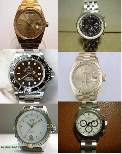
The major challenge when learning the structure of HCMs is that it requires the resolution of a fundamental chicken-and-egg problem: In order to learn the graph structure of an HCM the object must be segmented from the background, however, in order to segment the object from the background an object model is needed. Existing structure learning approaches resolve this problem by taking one of the following assumptions:
- A1
- A2
- A3
The assumptions A1 and A3 are unsatisfying as they require detailed human supervision during training. Assumption A2 does not hold in general for natural images because the appearance of objects is locally highly ambiguous [19]. When learning from natural images this leads to background structures becoming part of the object model, or object parts being missed in the representation [30].
The major contribution of this paper is a framework for learning the graph structure of hierarchical compositional models without relying on the assumptions A1-A3. In particular, we make the following contributions:
-
•
Generalized formulation of HCMs. We present a generalized formulation of hierarchical compositional models that allows for probabilistic modeling of objects with arbitrary numbers of parts.
-
•
Greedy structure learning framework. We propose a novel greedy learning framework for hierarchical compositional models. It consists of a bottom-up compositional clustering process that infers the number of parts per layer as well as the number of layers in a HCM. A subsequent top-down process composes the learned hierarchical parts into a holistic object model.
-
•
Background modeling in structure learning. We introduce a background model into the structure learning process and thus integrate the foreground-background segmentation task into the learning procedure. In this way, we can resolve the need for providing segmented training data.
-
•
Overcoming limitations of related work. Our qualitative results demonstrate that semantically meaningful HCMs are learned without relying on the assumptions A1-A3. Our quantitative experiments at transfer learning on the Four Domain dataset [12] show that our learned HCMs outperform other generative approaches in terms of classification accuracy.
2 Related Work
Deformable object models: Deformable object models explicitly represent an object in terms of a reference object and a model of how instances of the object can deform [14]. In their seminal work, Kaas et al. [18] proposed an approach for detecting deformable contours in images with a hand-designed deformation model. Cootes et al. [4] were the first to learn a statistical deformation model from data. Yuille et al. [36] proposed to relax the global dependence between different parts of the object by introducing a hierarchical model structure. In this way, the parts could move locally independently, while, a global energy term constrained the global structure of the model. Such tree-structured models can be optimized efficiently, and therefore gained significant momentum, leading to a body of work that has developed along this line of research [32, 7, 6, 17, 16, 27]. The Active Basis Model [34] is a deformable object model that is formulated within an elegant information-theoretic framework and, in addition to shape deformations, also models the object’s appearance. In this work, we use the hierarchical compositional generalization of the Active Basis Model [5] as object representation.
Hierarchical compositional models. Hierarchical compositional models have developed as a class of models which extend deformable templates into hierarchical graphs that explicitly allow for part sharing, and thus yield big gains in computational efficiency. Furthermore, they have proven to be highly robust under strong changes in the visual domain [37], while achieving state-of-the-art performance in several computer vision tasks [24, 38, 17, 31, 5, 29]. These approaches hand-specify the graph structures of the models and are restricted to learn the parameters only, whereas, in this work we propose to learn the graph structure from data.
Learning the structure of hierarchical compositional models. It is desirable to learn the structure of HCMs from data. A number of works [10, 9, 8, 20, 39] showed that exploiting the modularity of compositional models makes possible to learn HCMs one parent child clique at a time in a bottom-up manner by clustering contours. Recent work, on object recognition in changing visual environments [11, 21, kortylewski2017model] showed that HCMs are extremely data efficient while being highly adaptive to different visual domains. These methods, however, rely on segmented training data. In contrast, we propose to learn the structure and parameters of hierarchical compositional models from natural images without relying on detailed human supervision in terms of segmented training data or prior knowledge about the object’s geometry.
Background modeling for generative object models. When analyzing images with generative object models, the background is often not modeled explicitly but represented implicitly via detection thresholds or manually specified constraints on the range of model parameters [26]. In [34, 26] the authors propose to resolve such artificial constraints by letting an explicit background model compete with the generative object model (the foreground) in explaining a target image during inference. In this paper, we propose to integrate an explicit background model as competitor of the generative object model during learning. In this way, we integrate the foreground-background segmentation task into the learning process and thus overcome the need for detailed human supervision.
3 Theoretical background
In this section, we describe the theoretical details of our hierarchical compositional object model. We start by introducing the Active Basis Model (ABM, Section 3.1) and its compositional generalization (CABM, Section 3.2). Building on this theoretical background, we introduce the proposed generalized multi-layer CABM in Section 3.3.
3.1 Active Basis Model
ABMs [34] are probabilistic generative models that model an object’s variability in terms of shape and appearance. An ABM represents an image as a linear combination of basis filters :
| (1) |
The image is decomposed into a set of Gabor filters with fixed frequency band, coefficients and a residual image . The variable denotes the absolute position and orientation of a basis filter in the image frame. These parameters are encoded relative to the objects center such that . The superscripts of the parameters indicate the layer at which the variables are located in the graphical model of the ABM. This will become important when we discuss the hierarchical generalization of ABMs in the next section. The parameters of the filters can be learned with matching pursuit [23] from a set of training images as introduced in [34]. By inducing a probability distribution on the model parameters and a generative object model is defined:
| (2) |
The prior of the position and orientation of the object is simply uniformly distributed over all possible rotations and all positions in the image frame. The position of the individual filters varies locally according to a uniform distribution around the mean position of a filter with describing the possible spatial perturbation. The filter coefficients follow a statistical distribution in the form of an exponential family model:
| (3) |
where each filter coefficient is bounded with a sigmoid transform saturating at value , in order to prevent the overfitting of the model to strong edges. The natural parameter is learned from the training data via maximum-likelihood estimation and the normalizing constant can be estimated by integrating the numerator on a set of training images (more details on this process can be found in [34]). The core limitation of ABMs is that they assume statistical independence between individual basis filters (Eq. 2). Therefore they are limited in terms of their ability to model large object deformations and strong appearance changes [5]. In the next section, we introduce Compositional Active Basis Models [5] which overcome this limitation by introducing hierarchical relations between the basis filters.
3.2 Compositional Active Basis Model
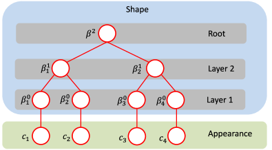
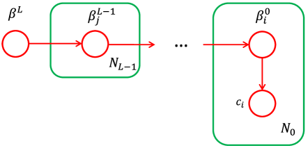
Figure 2a graphically illustrates the dependency structure of a two-layered Compositional Active Basis Model (CABM) as proposed by Dai et al. [5]. Note the tree-like dependency structure between the variables which enables a fast posterior inference via dynamic programming. The probabilistic image model of a two-layered CABM is defined as:
| (4) |
where the operator selects the set of children nodes. Compared to the original ABM (Equation 2), additional dependencies are introduced between group of the individual basis filters (). In this way, the object’s global structure is partitioned into multiple conditionally independent groups of basis filters. This allows for the modeling of long-range correlations in the object’s geometry which cannot be achieved with the standard ABM. The learning of CABMs was originally proposed in [5], however, the number of parts per layer was assumed to be known a-priori and the number of layers was fixed to 2 (see Figure 1b). In the next section, we present a generalization of the CABM which will enable us to overcome this assumption via a greedy structure learning framework in Section 4.
3.3 Proposed approach: Multi-Layer CABM
We can generalize the CABM model to an arbitrary numbers of hierarchical layers :
| (5) |
which corresponds to the graphical model shown in Figure 2b. Based on this multi-layer generalization the model becomes more expressive, and therefore can represent objects with very different geometry structure, such as e.g. long and thin objects as well as small but compact objects. In this way, we evade the need for specifying the dependency structure of the model a-priori, and thus overcome the main limitation of the original model [34] (compare Figures 1b and 1c with a specified and learned dependence structure, respectively). However, the additional model flexibility comes at the price of having to learn the full dependency structure of the probabilistic model, including the number of layers , the number of parts per layer and their hierarchical dependency structure. Note that Eq. (5) can be used to compute and compare posterior probabilities of models which are composed of different numbers of components. In the next section, we propose a greedy structure learning framework for estimating those parameters from data.
Input: Set of Gabor filters ;
. Set of training images
Output: Set of Hierarchical Compositional Part Models .
4 Greedy structure learning
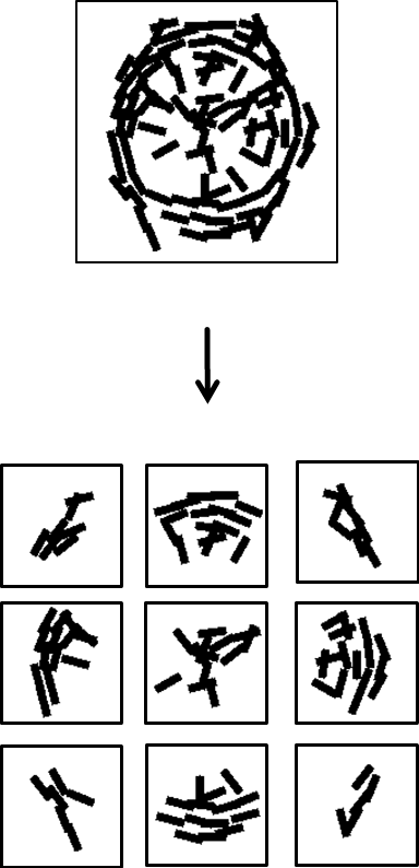
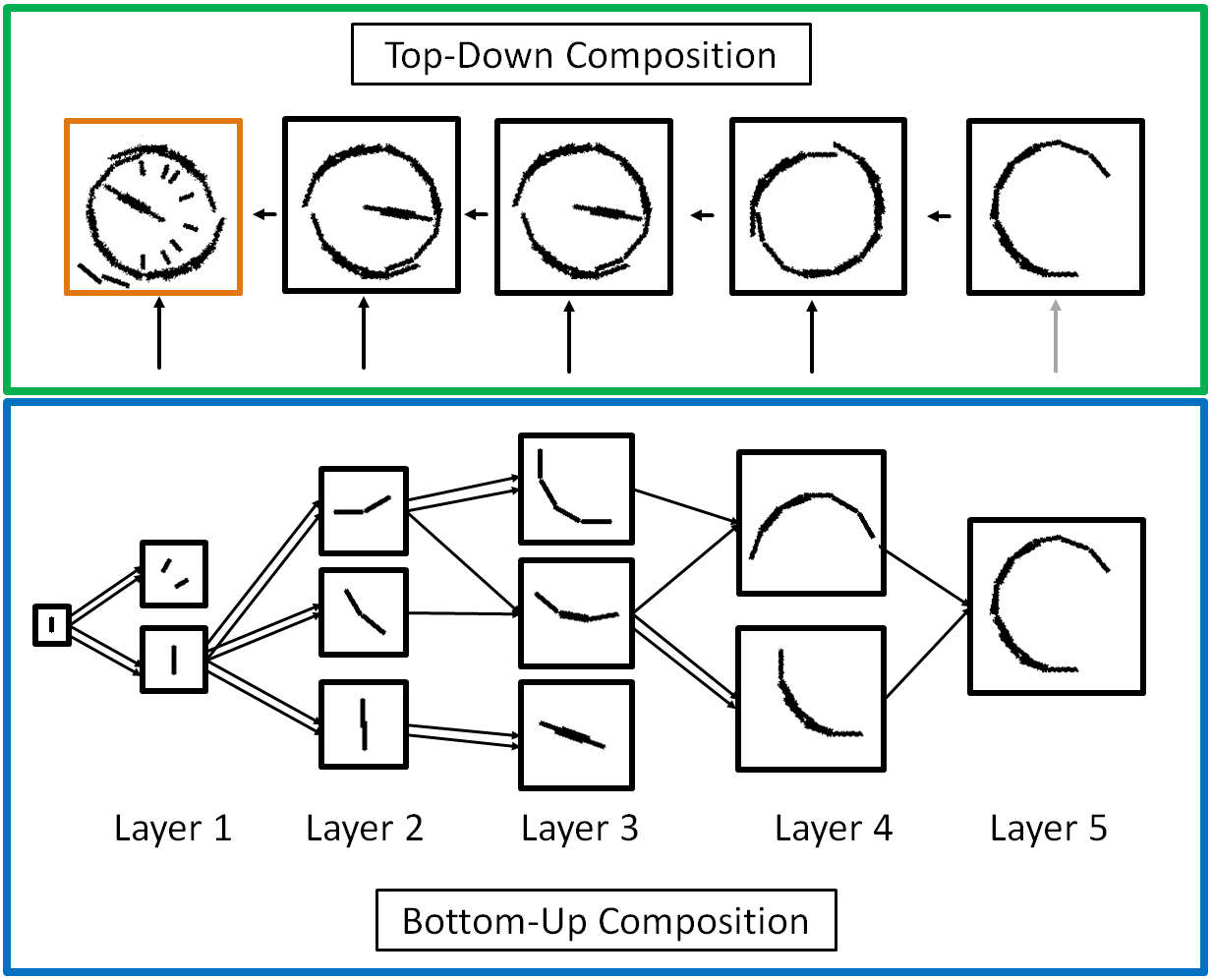
In this section, we describe a greedy structure learning algorithm that infers the full dependency structure of the multi-layer CABM from natural images. Figure 3 illustrates the two phases of this learning process: A bottom-up compositional clustering process (Figure 3 blue box) and a top-down model composition phase (Figure 3 green box). In the bottom-up process, the parts of lower layers in the hierarchy are learned first and subsequently composed into higher-order parts. The top-down process composes the (independent) hierarchical parts into a holistic object model. The following paragraphs describe both processes in detail.

4.1 Bottom-up compositional clustering
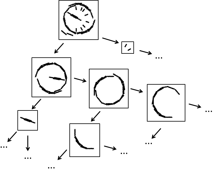
We propose to formulate the structure learning task as a compositional clustering process that is described in Algorithm 1. The dependence structure of our HCM is a tree-like Markov random field (Figure 2 & Equation 5). This enables us to learn the model in a bottom-up manner, i.e. we can learn the first-layer parts first, before proceeding to compose them into larger parts (Algorithm 1, lines ). At each layer of the hierarchy, the parts are learned according to a greedy EM-type learning scheme that infers the structure of each part as well as the number of part models from training images (Algorithm 1, line ).
Greedy EM-type learning. The general procedure of the proposed greedy learning scheme is described in (Algorithm 1, line ), while Figure 4a analogously illustrates a particular learning example. We first explain the algorithmic process and then comment on the visual illustration. The learning process is initialized with two part models () which are learned with matching pursuit [23] from image patches that are randomly sampled from the training data (Algorithm 1, line ). Subsequently an EM-type update scheme is performed (Algorithm 1, line ) as follows:
-
1.
Detection (E-step): Detect part models in the training images at different locations and orientations. Cut out patches at the detected positions which serve as new training data for the M-step (Algorithm 1, line ).
- 2.
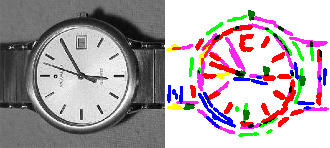
During the EM iterations we only update one part model () while the other model () stays fixed to its initial state and only participates in the detection phase. In doing so, it serves as a generic background model preventing from explaining image patches for which the normalized posterior is smaller than (analogous to Equation 5 and Figure 2b). This mechanism supports in specializing to a particular image structure (see e.g. the ticks of the watch in Figure 3) by explaining away irrelevant data (e.g. patches sampled from background clutter). After a fixed number of iterations and two new part models and are added to the model pool (Algorithm 1, line ). This time, however, the training patches are not sampled randomly, but inversely proportional to the marginal posterior . In this way, those regions which are well explained by the already learned model , are less likely to be sampled as training data for the new models. In the following iterations, is updated in the learning phase, while and serve as competitors, explaining away irrelevant training patches in the detection phase. The learning proceeds until iteration is converged. This greedy learning scheme repeats until a newly initialized model is not able to explain training patches better than any previously learned model or the background model (Algorithm 1, line ).
Figure 4a analogously illustrates the first iterations of such a greedy EM-type learning scheme. In the illustrated example, first-layer parts are learned to be composed of five Gabor filters (colored ellipses). We can observe that the learned models specialize to a particular local image structure, while the background models (dashed rectangles) have a rather random structure. Figure 4b illustrated an encoding of a training image with the final set of part models . Note how different models have specialized to different parts of the watch.
Bottom-up learning. After the parts of the first layer are learned, the structure induction process continues by composing the elements of into parts of the second layer . Thereby, we follow the same greedy EM-type learning process. This time, however, instead of composing single basis filter, the algorithm composes the elements of into higher order parts. We repeat the compositional learning iteratively layer by layer until the normalized model posterior does not increase anymore (Algorithm 1, line ), thus generating dictionaries of hierarchical part models at each layer of the hierarchy (Figure 3, blue box).
4.2 Top-down model building
After the bottom-up learning process, the learned part dictionaries must be composed into a holistic object model (Figure 3, green box). Note that different parts of an object can terminate at different layers of the hierarchy. For example, the hour markings on the dial of the watch in Figure 3 (orange box) are represented at the second layer, whereas, the circular shape of the watch is composed of more elements and is therefore represented at a higher layer. We suggest a top-down model building process for learn the dependency structure of the complete object, we introduce a top-down model building process.
The training images are first aligned, by detecting the part model of the highest layer in all training images followed by aligning the images such that the models are in a canonical orientation and position. After this alignment step, we proceed in a top-down manner (green box in Figure 3), adding parts from the highest layer to the object model with matching pursuit. We iteratively proceed layer-wise until the bottom layer of the hierarchy. At this point, we have learned a hierarchical compositional object model from natural images (orange box in Figure 3). Note that the number of layers , the number of parts per layer and the hierarchical dependency structure have been learned from natural images without restricting the object’s geometry or requiring segmented training data.
| Methods | C A | C D | A C | A W | W C | W A | D A | D W |
| KSVD [1] | 20.5 0.8 | 19.8 1.0 | 20.2 0.9 | 16.9 1.0 | 13.2 0.6 | 14.2 0.7 | 14.3 0.3 | 46.8 0.8 |
| SGF [13] | 36.8 0.5 | 32.6 0.7 | 35.3 0.5 | 31.0 0.7 | 21.7 0.4 | 27.5 0.5 | 32.0 0.4 | 66.0 0.5 |
| HABM [5] | 53.7 4.7 | 43.2 4.9 | 41.2 1.6 | 28.1 2.0 | 25.8 1.6 | 33.5 2.9 | 34.6 3.7 | 68.2 2.9 |
| OURS | 62.3 3.4 | 43.7 2.9 | 54.0 2.4 | 33.3 1.7 | 29.5 1.1 | 35.0 3.6 | 33.1 2.4 | 65.6 3.8 |
| Methods | C A | C D | A C | A W | W C | W A | D A | D W |
|---|---|---|---|---|---|---|---|---|
| Metric [25] | 33.7 0.8 | 35.0 1.1 | 27.3 0.7 | 36.0 1.0 | 21.7 0.5 | 32.3 0.8 | 30.3 0.8 | 55.6 0.7 |
| SGF [13] | 40.2 0.7 | 36.6 0.8 | 37.7 0.5 | 37.9 0.7 | 29.2 0.7 | 38.2 0.6 | 39.2 0.7 | 69.5 0.9 |
| FDDL [35] | 39.3 2.9 | 55.0 2.8 | 24.3 2.2 | 50.4 3.5 | 22.9 2.6 | 41.1 2.6 | 36.7 2.5 | 65.9 4.9 |
| HMP [3] | 67.7 2.3 | 70.2 5.1 | 51.7 4.3 | 70.0 4.2 | 46.8 2.1 | 61.5 3.8 | 64.7 2 | 76.0 4 |
| SDDL [28] | 49.5 2.6 | 76.7 3.9 | 27.4 2.4 | 72.0 4.8 | 29.7 1.9 | 49.4 2.1 | 48.9 3.8 | 72.6 2.1 |
| HABM [5] | 68.3 2.3 | 57.4 6.0 | 52.7 3.0 | 54.8 2.8 | 42.2 3.1 | 57.1 3.5 | 60.1 3.2 | 79.7 2.5 |
| OURS | 72.2 0.7 | 58.1 5.1 | 58.5 1.2 | 53.4 1.2 | 47.6 1.8 | 61.7 3.2 | 65.6 2.8 | 78.5 2.0 |
5 Results
We evaluate the proposed HCM learning scheme qualitatively by comparing it to the HABM approach proposed in [5]. Quantitative results are presented at the task of domain adaptation on the Four Domain Dataset [12] and compared to other generative approaches. Note that it is difficult to evaluate generative object models at object recognition tasks, as they are optimized via a data reconstruction criterion and thus naturally perform worse than methods which are directly optimized via a discriminative criterion. Furthermore, generative models provide a manifold of information in addition to the mere class label, such as e.g. the position of the object, detailed part annotations and a foreground-background segmentation.
Parameter settings. In our experiments, the images have a mean height of pixels while a Gabor filter has a quadratic size of pixels. The Gabor filters and higher layer parts are rotated in 10 degree steps. We found empirically that in the greedy learning scheme, a part model is converged to stable solution after learning iterations. The hierarchical graph structure is defined to compose two parts at each layer of the hierarchy. Changing the number of parts to be composed at each layer would have implications on the overall number of layers learned during training, however, we found that it has no particular impact on the overall performance in the quantitative experiments.


5.1 Visual Domain Adaptation
We follow the common evaluation protocol of using generative part-based models as feature extractors for discriminative methods. The rationale behind this setup is that generative models are highly adaptive to changes in the visual environment and thus are suited as feature extractors for domain adaptation tasks. We evaluate our approach on the Four Domain Dataset [12], which is composed of identical classes from the following datasets: Amazon with images downloaded from Amazon; DSLR with high-resolution images; Webcam with low-resolution images and images from Caltech256 [15]. In each dataset, the image resolution, lighting conditions, background, the object textures and positions in space vary significantly. We follow the standard evaluation protocol as introduced in [12]. We test two experimental setups: In the semi-supervised setting, the algorithm has access to a small amount of data from the target domain, whereas in the unsupervised setting the training images are only sampled from the source domain. As proposed in [5], we use the learned HCM as feature extractor for a spatial pyramid matching [22]. A multi-class SVM is trained on the extracted features and used for classification. The classification results in Tables 1 & 2 show that:
Our approach outperforms other generative methods at the task of unsupervised domain adaptation (Table 1). Note that our method uses exactly the same Gabor basis as the HABM. The performance increase can be attributed to the fact that we learn the hierarchical structure and do not specify it a-priori as in the HABM. Interestingly, our approach is outperformed by HABM when learning from the DSLR dataset, which has a strong intra-domain viewpoint variation. As we enforce the learning of a single holistic object model, our approach specializes to one of the viewpoints, whereas, in the HABM method multiple templates are learned. Note that our approach could in principle be extended to multi-object learning.
Our models achieve the best performance in most experiments in the semi-supervised setting (Table 2). Again we outperform the HABM approach in most experiments. Interestingly, the performance gap between our method and HABM when learning from DSLR is essentially closed in the semi-supervised setting. The reason is that the objects in the Amazon and Webcam class have significantly less variation in the viewpoint. Our learning scheme can leverage this and will specialize to the most common viewpoint in the data. Therefore, the advantage of having multiple templates in the HABM is reduced.
5.2 Qualitative Evaluation
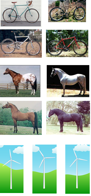
Our approach learns the structure of HCMs from natural images. The learning results of Figure 5b & 5c demonstrate that our approach is able to learn the hierarchical structure of HCMs from cluttered natural images. Importantly, our approach does not depend on detailed human supervision during learning. This is in contrast to prior work that relies on detailed object segmentations [11, 21] or a-priori knowledge about the hierarchical structure [5, 39].
Our HCMs are more efficient and semantically more meaningful compared to prior work. Learning the full hierarchical structure enables the reuse of parts within the hierarchy (e.g. the wheels of the bike in Figure 5c), which is not possible in the HABM approach [5] (Figure 5d). Therefore, our HCMs have semantically more meaningful parts that provide additional information about the internal semantics of the object. Furthermore, our learning process is more data efficient as the part models can leverage the redundancy within objects (e.g. if the same part occurs multiple times within the same object).
A limitation of our approach and any prior work, including HABM, is that so far it is not possible to learn HCMs of articulated objects (e.g. the windmill in Figure 5). Although the individual parts of the windmill are learned by our bottom-up process (Figure 5b), the top-down process cannot compose the parts into a holistic object model as our deformation model assumes that the relative orientation between parts of an object stays approximately the same.
6 Conclusion
In this work, we considered the challenging problem of learning a hierarchical generative model of an object from only a set of images which show examples of the object in the presence of variable background clutter. In this context, we made the following contributions:
Multi-layer Compositional Active Basis Models (CABMs). Building on related work, we proposed a generalized probabilistic formulation of CABMs with arbitrary numbers of layers and parts per layer. Our model is more flexible and enables the representation of objects with very different geometry structures. It also opens the possibility to learn hierarchical object representations which efficiently re-use parts and thus provide rich information about the objects internal structure (Fig. 1c & 5).
Structure learning from cluttered data. We introduced a framework for learning the structure of multi-layer CABMs from natural images based on class labels only. Notably, we were able to learn the full dependency structure, including the number of layers in the hierarchy and the number of parts per layer, despite complex variations in the images, in terms of highly variable background clutter and object appearance. Importantly, our framework overcomes the limitations of related works which either require segmented training data or make too strong assumptions about the object’s geometry. The learned models also outperformed other generative object models at object classification on a standard domain transfer dataset.
Acknowledgements: A.K. is supported by the Novartis University of Basel Excellence Scholarship for Life Sciences and the SNSF grant P2BSP2_181713. A.W., M.W., S.P. are partially supported by the NCCR MARVEL and SNSF grants CR32I2159682 and 51MRP0158328.
References
- [1] Aharon, M., Elad, M., Bruckstein, A.: K-svd: An algorithm for designing overcomplete dictionaries for sparse representation. Signal Processing, IEEE Transactions on 54(11), 4311–4322 (2006)
- [2] Blanz, V., Vetter, T.: A morphable model for the synthesis of 3d faces. In: Proceedings of the 26th annual conference on Computer graphics and interactive techniques, pp. 187–194. ACM Press/Addison-Wesley Publishing Co. (1999)
- [3] Bo, L., Ren, X., Fox, D.: Hierarchical matching pursuit for image classification: Architecture and fast algorithms. In: Advances in neural information processing systems, pp. 2115–2123 (2011)
- [4] Cootes, T.F., Taylor, C.J., Cooper, D.H., Graham, J.: Active shape models-their training and application. Computer vision and image understanding 61(1), 38–59 (1995)
- [5] Dai, J., Hong, Y., Hu, W., Zhu, S.C., Wu, Y.N.: Unsupervised learning of dictionaries of hierarchical compositional models. In: Computer Vision and Pattern Recognition (CVPR), 2014 IEEE Conference on, pp. 2505–2512. IEEE (2014)
- [6] Epshtein, B., Uliman, S.: Feature hierarchies for object classification. In: Computer Vision, 2005. ICCV 2005. Tenth IEEE International Conference on, vol. 1, pp. 220–227. IEEE (2005)
- [7] Felzenszwalb, P.F., Huttenlocher, D.P.: Pictorial structures for object recognition. International journal of computer vision 61(1), 55–79 (2005)
- [8] Ferrari, V., Jurie, F., Schmid, C.: From images to shape models for object detection. International journal of computer vision (2010)
- [9] Fidler, S., Boben, M., Leonardis, A.: Learning a hierarchical compositional shape vocabulary for multi-class object representation. arXiv preprint arXiv:1408.5516 (2014)
- [10] Fidler, S., Leonardis, A.: Towards scalable representations of object categories: Learning a hierarchy of parts. In: Computer Vision and Pattern Recognition, 2007. CVPR’07. IEEE Conference on, pp. 1–8. IEEE (2007)
- [11] George, D., Lehrach, W., Kansky, K., Lázaro-Gredilla, M., Laan, C., Marthi, B., Lou, X., Meng, Z., Liu, Y., Wang, H., et al.: A generative vision model that trains with high data efficiency and breaks text-based captchas. Science 358(6368), eaag2612 (2017)
- [12] Gong, B., Shi, Y., Sha, F., Grauman, K.: Geodesic flow kernel for unsupervised domain adaptation. In: Computer Vision and Pattern Recognition (CVPR), 2012 IEEE Conference on, pp. 2066–2073. IEEE (2012)
- [13] Gopalan, R., Li, R., Chellappa, R.: Domain adaptation for object recognition: An unsupervised approach. In: ICCV (2011)
- [14] Grenander, U.: Elements of pattern theory. JHU Press (1996)
- [15] Griffin, G., Holub, A., Perona, P.: Caltech-256 object category dataset (2007)
- [16] Hinton, G.E., Osindero, S., Teh, Y.W.: A fast learning algorithm for deep belief nets. Neural computation 18(7), 1527–1554 (2006)
- [17] Jin, Y., Geman, S.: Context and hierarchy in a probabilistic image model. In: Computer Vision and Pattern Recognition, 2006 IEEE Computer Society Conference on, vol. 2, pp. 2145–2152. IEEE (2006)
- [18] Kass, M., Witkin, A., Terzopoulos, D.: Snakes: Active contour models. International journal of computer vision 1(4), 321–331 (1988)
- [19] Kersten, D., Yuille, A.: Bayesian models of object perception. Current opinion in neurobiology 13(2), 150–158 (2003)
- [20] Kokkinos, I., Yuille, A.: Inference and learning with hierarchical shape models. International Journal of Computer Vision 93(2), 201–225 (2011)
- [21] Kortylewski, A., Vetter, T.: Probabilistic compositional active basis models for robust pattern recognition. In: BMVC (2016)
- [22] Lazebnik, S., Schmid, C., Ponce, J.: Beyond bags of features: Spatial pyramid matching for recognizing natural scene categories. In: Computer Vision and Pattern Recognition, 2006 IEEE Computer Society Conference on, vol. 2, pp. 2169–2178. IEEE (2006)
- [23] Mallat, S.G., Zhang, Z.: Matching pursuits with time-frequency dictionaries. Signal Processing, IEEE Transactions on 41(12), 3397–3415 (1993)
- [24] Ommer, B., Buhmann, J.M.: Learning the compositional nature of visual object categories for recognition. Pattern Analysis and Machine Intelligence, IEEE Transactions on 32(3), 501–516 (2010)
- [25] Saenko, K., Kulis, B., Fritz, M., Darrell, T.: Adapting visual category models to new domains. In: Computer Vision–ECCV 2010, pp. 213–226. Springer (2010)
- [26] Schönborn, S., Egger, B., Forster, A., Vetter, T.: Background modeling for generative image models. Computer Vision and Image Understanding 136, 117–127 (2015)
- [27] Serre, T., Wolf, L., Bileschi, S., Riesenhuber, M., Poggio, T.: Robust object recognition with cortex-like mechanisms. Pattern Analysis and Machine Intelligence, IEEE Transactions on 29(3), 411–426 (2007)
- [28] Shekhar, S., Patel, V., Nguyen, H., Chellappa, R.: Generalized domain-adaptive dictionaries. In: Proceedings of the IEEE Conference on Computer Vision and Pattern Recognition, pp. 361–368 (2013)
- [29] Si, Z., Zhu, S.C.: Learning and-or templates for object recognition and detection. Pattern Analysis and Machine Intelligence, IEEE Transactions on 35(9), 2189–2205 (2013)
- [30] Spehr, J.: On Hierarchical Models for Visual Recognition and Learning of Objects, Scenes, and Activities, vol. 11. Springer (2014)
- [31] Todorovic, S., Ahuja, N.: Unsupervised category modeling, recognition, and segmentation in images. Pattern Analysis and Machine Intelligence, IEEE Transactions on 30(12), 2158–2174 (2008)
- [32] Weber, M., Welling, M., Perona, P.: Unsupervised learning of models for recognition. In: European conference on computer vision, pp. 18–32. Springer (2000)
- [33] Wong, A., Yuille, A.: One shot learning via compositions of meaningful patches. In: ICCV (2015)
- [34] Wu, Y.N., Si, Z., Gong, H., Zhu, S.C.: Learning active basis model for object detection and recognition. International journal of computer vision 90(2), 198–235 (2010)
- [35] Yang, M., Zhang, L., Feng, X., Zhang, D.: Fisher discrimination dictionary learning for sparse representation. In: ICCV (2011)
- [36] Yuille, A.L., Hallinan, P.W., Cohen, D.S.: Feature extraction from faces using deformable templates. International journal of computer vision 8(2), 99–111 (1992)
- [37] Yuille, A.L., Liu, C.: Deep nets: What have they ever done for vision? arXiv preprint arXiv:1805.04025 (2018)
- [38] Zhu, L., Chen, Y., Yuille, A.: Learning a hierarchical deformable template for rapid deformable object parsing. Pattern Analysis and Machine Intelligence, IEEE Transactions on 32(6), 1029–1043 (2010)
- [39] Zhu, L.L., Lin, C., Huang, H., Chen, Y., Yuille, A.: Unsupervised structure learning: Hierarchical recursive composition, suspicious coincidence and competitive exclusion. In: Computer vision–eccv 2008, pp. 759–773. Springer (2008)
- [40] Zhu, S.C., Mumford, D., et al.: A stochastic grammar of images. Foundations and Trends® in Computer Graphics and Vision 2(4), 259–362 (2007)