Estimation of the shape of the density contours of star-shaped distributions

Abstract

Elliptically contoured distributions generalize the multivariate normal distributions in such a way that the density generators need not be exponential. However, as the name suggests, elliptically contoured distributions remain to be restricted in that the similar density contours ought to be elliptical. Kamiya, Takemura and Kuriki [Star-shaped distributions and their generalizations, Journal of Statistical Planning and Inference 138 (2008), 3429–3447] proposed star-shaped distributions, for which the density contours are allowed to be boundaries of arbitrary similar star-shaped sets. In the present paper, we propose a nonparametric estimator of the shape of the density contours of star-shaped distributions, and prove its strong consistency with respect to the Hausdorff distance. We illustrate our estimator by simulation.

Key words: density contour, direction, elliptically contoured distribution, Hausdorff distance, kernel density estimator, star-shaped distribution, strong consistency.

MSC2010: 62H12, 62H11, 62G07.

1 Introduction

Elliptically contoured distributions generalize the multivariate normal distributions in such a way that the density generators need not be exponential (Fang and Zhang [2]). In this way, the class of elliptically contoured distributions includes, for example, distributions whose tails are heavier than those of the multivariate normal distributions. However, as the name suggests, elliptically contoured distributions remain to be restricted in that the similar density contours ought to be elliptical. Hence, in particular, no skewed distributions are members of this class. Skew-elliptical distributions (Genton [4]) allow skewness by introducing an extra parameter into elliptically contoured distributions.

Kamiya, Takemura and Kuriki [7] proposed a flexible class of distributions called star-shaped distributions, for which the density contours are allowed to be boundaries of arbitrary similar star-shaped sets (see also [9], [6]). Essentially the same idea can be found in $v$-spherical distributions by Fernández, Osiewalski and Steel [3] and center-similar distributions by Yang and Kotz [10]. Skewness as well as heavy-tailedness is allowed in star-shaped distributions. Thus, besides (centrally, reflectively or in some other ways) symmetric distributions such as elliptically contoured distributions and $l_{q}$-spherical distributions, the class of star-shaped distributions also includes asymmetric distributions.

Kamiya, Takemura and Kuriki [7] studied distributional properties of star-shaped distributions, including independence of the “length” and the “direction,” and robustness of the distribution of the “direction.” However, they did not explore inferential aspects of star-shaped distributions. From the perspective of [7], the most important problem in the inference for star-shaped distributions is the estimation of the shape of the density contours.

In the present paper, we propose a nonparametric estimator of the shape of the density contours. The point is that the density of the usual direction under a star-shaped distribution is in one-to-one correspondence with a function which determines the shape of the density contours. Thus, by nonparametrically estimating the density of the direction, we can obtain a nonparametric estimator of the shape. We prove its strong consistency with respect to the Hausdorff distance.

In a recent paper, Liebscher and Richter [8] presented examples of parametric modeling and estimation concerning the shape of the density contours of two-dimensional star-shaped distributions (Section 2.2 as well as Sections 3.3 and 3.4 of [8]). They also investigated estimation about many other aspects of star-shaped distributions.

The organization of this paper is as follows. We describe a star-shaped distribution and define the shape of its density contours in Section 2. Next, we propose an estimator of the shape of the density contours of a star-shaped distribution in Section 3.1, and prove its strong consistency in Section 3.2. We illustrate our estimator by simulation in Section 4, and conclude with some remarks in Section 5.

2 Star-shaped distribution and the shape of its density contours

In this section, we describe a star-shaped distribution and define the shape of its density contours.

Suppose a random vector $x\in{\cal X}:={\mathbb{R}}^{p}\setminus\{{\bf 0}\},\ p\geq 2$, is distributed as

(1) $$x\sim h(r(x))dx,$$

where $r:{\cal X}\to{\mathbb{R}}_{>0}$ is continuous and equivariant under the action of the positive real numbers: $r(cx)=cr(x)$ for all $c\in{\mathbb{R}}_{>0}$. In (1), it is implicitly assumed that $h:{\mathbb{R}}_{>0}\to{\mathbb{R}}_{\geq 0}$ satisfies $0<\int_{0}^{\infty}h(r)r^{p-1}dr<\infty$. In the particular case that $r(x)=(x^{T}\Sigma^{-1}x)^{1/2}$ for a positive definite matrix $\Sigma$ ($x^{T}$ denotes the transpose of the column vector $x$) and that the density generator $h((-2(\,\cdot\,))^{1/2})$ is exponential: $h((-2(\,\cdot\,))^{1/2})\propto\exp(\,\cdot\,)$, we obtain the multivariate normal distribution $N_{p}({\bf 0},\Sigma)$.

Define

(2) $$Z:=\left\{x\in{\cal X}:r(x)=1\right\},$$

and write $cZ:=\{cz:z\in Z\}$ for $c\in{\mathbb{R}}_{\geq 0}$. Then the density $h(r(x))$ is constant on each of $cZ\subset{\cal X},\ c\in{\mathbb{R}}_{>0}$: $h(r(x))=h(c)$ for all $x\in cZ$. When $h:{\mathbb{R}}_{>0}\to{\mathbb{R}}_{\geq 0}$ is injective (e.g., strictly decreasing), each $cZ,\ c\in{\mathbb{R}}_{>0}$, is a contour of the density $h(r(x))$: $cZ=\{x\in{\cal X}:h(r(x))=h(c)\}$, but in general, a contour of the density is a union of some $cZ$’s: $\{x\in{\cal X}:h(r(x))=t\}=\bigcup_{c\in h^{-1}(\{t\})}cZ,\ t\in{\mathbb{R}}_{\geq 0}$.

Noticing that ${\cal Z}:=\bigcup_{0\leq c\leq 1}cZ\subset{\cal X}\cup\{{\bf 0}\}={\mathbb{R}}^{p}$ is a star-shaped set with respect to the origin, we say that $x$ in (1) has a star-shaped distribution. Also, we call $Z$ the shape of the density contours of this star-shaped distribution, including cases where $h$ is not injective. When $h$ is strictly decreasing, ${\cal Z}$ is a density level set: ${\cal Z}=\{x\in{\cal X}:h(r(x))\geq h(1)\}\cup\{{\bf 0}\}$.

The focus of this paper is the estimation of the shape $Z$ in (2). In the next section, we propose an estimator of the form

$$\left\{\hat{f}_{n}(u)^{\frac{1}{p}}u:u\in{\mathbb{S}}^{p-1}\right\},$$

where ${\mathbb{S}}^{p-1}$ is the unit sphere in ${\mathbb{R}}^{p}$ and $\hat{f}_{n}(u)$ is a directional density estimator based on the directions of a sample from (1).

3 Estimation of the shape

In this section, we propose an estimator of the shape of the density contours of a star-shaped distribution (Section 3.1), and prove its strong consistency (Section 3.2).

3.1 Proposed estimator

In this subsection, we propose an estimator of the shape $Z$.

Let $\|\cdot\|$ denote the Euclidean norm. Under (1), the direction $u:=x/\|x\|\in{\mathbb{S}}^{p-1}$ is distributed as

(3) $$u\sim f(u)du\text{ \quad with \ }f(u):=c_{0}r(u)^{-p},$$

where $du$ stands for the volume element of ${\mathbb{S}}^{p-1}$ and $c_{0}=1/\int_{{\mathbb{S}}^{p-1}}r(u)^{-p}du=\int_{0}^{\infty}h(r)r^{p-1}dr$ (Theorem 4.1 of [7]). Note the function $f:{\mathbb{S}}^{p-1}\to{\mathbb{R}}_{\geq 0}$ in (3) is continuous and satisfies $f(u)>0$ for all $u\in{\mathbb{S}}^{p-1}$. Throughout this section (Section 3), we assume $r(\,\cdot\,)$ is taken so that $\int_{{\mathbb{S}}^{p-1}}r(u)^{-p}du=1$ and hence $c_{0}=1$.

Now, we can write $r(u)=f(u)^{-1/p}$ for $u\in{\mathbb{S}}^{p-1}$. Thus, for $x\in{\cal X}$, the condition that $r(x)=1$ is equivalent to $\|x\|=1/r(x/\|x\|)=f(x/\|x\|)^{1/p}$. Hence $Z=\{x\in{\cal X}:r(x)=1\}=\{f(u)^{1/p}u:u\in{\mathbb{S}}^{p-1}\}$, and we can estimate $Z$ by estimating the density $f(u)$ of $u=x/\|x\|$.

Suppose we are given an i.i.d. sample $x_{1},\ldots,x_{n}$ from (1), and consider estimating $f(u)$ based on $u_{1},\ldots,u_{n}$, where $u_{i}:=x_{i}/\|x_{i}\|,\ i=1,\ldots,n$.

Let $\hat{f}_{n}(u)$ be an estimator of $f(u)$ such that $\hat{f}_{n}(u)\geq 0$ for all $u\in{\mathbb{S}}^{p-1}$. Define the estimator $\hat{Z}_{n}$ of $Z$ by

$$\hat{Z}_{n}:=\left\{\hat{f}_{n}(u)^{\frac{1}{p}}u:u\in{\mathbb{S}}^{p-1}\right\}.$$

Then $\hat{{\cal Z}}_{n}:=\bigcup_{0\leq c\leq 1}c\hat{Z}_{n}$ is also a star-shaped set with respect to the origin.

3.2 Strong consistency

In this subsection, we prove strong consistency of our estimator $\hat{Z}_{n}$.

Let $\delta_{H}(\hat{Z}_{n},Z)$ be the Hausdorff distance between $\hat{Z}_{n}$ and $Z$:

$$\delta_{H}(\hat{Z}_{n},Z):=\inf\left\{\delta>0:\hat{Z}_{n}\subset Z+B(\delta),\ Z\subset\hat{Z}_{n}+B(\delta)\right\},$$

where $B(\delta):=\{x\in{\mathbb{R}}^{p}:\|x\|\leq\delta\}$, and $+$ denotes the Minkowski sum. Similarly, let $\delta_{H}(\hat{{\cal Z}}_{n},{\cal Z})=\inf\{\delta>0:\hat{{\cal Z}}_{n}\subset{\cal Z}+B(\delta),\ {\cal Z}\subset\hat{{\cal Z}}_{n}+B(\delta)\}$ be the Hausdorff distance between $\hat{{\cal Z}}_{n}$ and ${\cal Z}$. We note that $\hat{Z}_{n}$ and $\hat{{\cal Z}}_{n}$ may not be compact. The purpose of this section is to show that, under some conditions, $\delta_{H}(\hat{Z}_{n},Z)$ and $\delta_{H}(\hat{{\cal Z}}_{n},{\cal Z})$ converge to zero almost surely.

We begin by proving that $\delta_{H}(\hat{Z}_{n},Z)$ and $\delta_{H}(\hat{{\cal Z}}_{n},{\cal Z})$ are bounded by $d_{n}:=\sup_{u\in{\mathbb{S}}^{p-1}}|\hat{f}_{n}(u)^{1/p}-f(u)^{1/p}|$:

(4) $$\delta_{H}(\hat{Z}_{n},Z)\leq d_{n},\qquad\delta_{H}(\hat{{\cal Z}}_{n},{\cal Z})\leq d_{n}.$$

Let $z_{0}=\tilde{c}_{0}f(u_{0})^{1/p}u_{0}$ $(0\leq\tilde{c}_{0}\leq 1,\ u_{0}\in{\mathbb{S}}^{p-1})$ be an arbitrary point of ${\cal Z}$. Take $z^{\prime}_{0}=\tilde{c}_{0}\hat{f}_{n}(u_{0})^{1/p}u_{0}\in\hat{{\cal Z}}_{n}$. Then $\|z^{\prime}_{0}-z_{0}\|=\tilde{c}_{0}|\hat{f}_{n}(u_{0})^{1/p}-f(u_{0})^{1/p}|\leq d_{n}$, and thus $z_{0}\in\hat{{\cal Z}}_{n}+B(d_{n})$. This argument implies that ${\cal Z}\subset\hat{{\cal Z}}_{n}+B(d_{n})$. Similarly, $\hat{{\cal Z}}_{n}\subset{\cal Z}+B(d_{n})$ holds true. Therefore, the second inequality in (4) is proved. The proof of the first inequality in (4) is similar.

Next we want to verify that $d_{n}\to 0$ almost surely for estimators $\hat{f}_{n}(u)$ having a certain property.

For each $u\in{\mathbb{S}}^{p-1}$ and each $n$, we can write

(5) $$\hat{f}_{n}(u)^{\frac{1}{p}}=f(u)^{\frac{1}{p}}+\frac{1}{p}f^{*}_{n}(u)^{\frac{1}{p}-1}\left(\hat{f}_{n}(u)-f(u)\right)$$

for some $f^{*}_{n}(u)$ between $\hat{f}_{n}(u)$ and $f(u)$.

Let $\epsilon_{n}:=\sup_{u\in{\mathbb{S}}^{p-1}}|\hat{f}_{n}(u)-f(u)|$. Then we have $f^{*}_{n}(u)\geq f(u)-\epsilon_{n}$ for all $u\in{\mathbb{S}}^{p-1}$ and all $n$, and thus

(6) $$\inf_{u\in{\mathbb{S}}^{p-1}}f^{*}_{n}(u)\geq\inf_{u\in{\mathbb{S}}^{p-1}}f(u)-\epsilon_{n}$$

for all $n$. Since $f:{\mathbb{S}}^{p-1}\to{\mathbb{R}}_{\geq 0}$ is continuous, ${\mathbb{S}}^{p-1}$ is compact and $f(u)>0$ for all $u\in{\mathbb{S}}^{p-1}$, we have $c_{f}:=\inf_{u\in{\mathbb{S}}^{p-1}}f(u)=\min_{u\in{\mathbb{S}}^{p-1}}f(u)>0$. Now, suppose the estimator $\hat{f}_{n}(u)$ satisfies

(7) $$\epsilon_{n}=\sup_{u\in{\mathbb{S}}^{p-1}}\left|\hat{f}_{n}(u)-f(u)\right|\to 0\quad{\rm a.s.}$$

Then, with probability one, we have $\epsilon_{n}<c_{f}/2$ for all sufficiently large $n$. Together with this fact, inequality (6) implies that, with probability one,

(8) $$\inf_{u\in{\mathbb{S}}^{p-1}}f^{*}_{n}(u)\geq c_{f}-\epsilon_{n}>\frac{c_{f}}{2}$$

for all sufficiently large $n$.

It follows from (5) and (8) that, with probability one,

$$d_{n}=\sup_{u\in{\mathbb{S}}^{p-1}}\left|\hat{f}_{n}(u)^{\frac{1}{p}}-f(u)^{\frac{1}{p}}\right| \leq \frac{1}{p}\left\{\inf_{u\in{\mathbb{S}}^{p-1}}f^{*}_{n}(u)\right\}^{\frac{1}{p}-1}\cdot\sup_{u\in{\mathbb{S}}^{p-1}}\left|\hat{f}_{n}(u)-f(u)\right|$$

$$\leq \frac{1}{p}\left(\frac{c_{f}}{2}\right)^{\frac{1}{p}-1}\epsilon_{n}$$

for all sufficiently large $n$. Therefore, by (7) we obtain $d_{n}\to 0\ {\rm a.s.}$, as was to be verified.

Now, for estimating a general density $f(u)$ on ${\mathbb{S}}^{p-1},\ p\geq 2$ (i.e., not necessarily $f(u)$ in (3)) based on an i.i.d. sample $u_{1},\ldots,u_{n}$ from $f(u)du$, we can use the following kernel density estimator (Hall, Watson and Cabrera [5], Bai, Rao and Zhao [1]):

(9) $$\hat{f}_{n}(u)=\frac{C(\eta)}{n\eta^{p-1}}\sum_{i=1}^{n}L\left(\frac{1-u^{T}u_{i}}{\eta^{2}}\right),\quad u\in{\mathbb{S}}^{p-1},$$

where $\eta=\eta_{n}>0$, $C(\eta):=\eta^{p-1}/\int_{{\mathbb{S}}^{p-1}}L((1-u^{T}y)/\eta^{2})du>0$ ($y\in{\mathbb{S}}^{p-1}$), and $L:{\mathbb{R}}_{\geq 0}\to{\mathbb{R}}_{\geq 0}$ satisfies $0<\int_{0}^{\infty}L(s)s^{(p-3)/2}ds<\infty$. Notice that $C(\eta)$ does not depend on $y$ and can be written as $C(\eta)=\eta^{p-1}/\{\omega_{p-1}\int_{-1}^{1}L((1-t)/\eta^{2})(1-t^{2})^{(p-3)/2}dt\}=1/\{\omega_{p-1}\int_{0}^{2/\eta^{2}}L(s)s^{(p-3)/2}(2-\eta^{2}s)^{(p-3)/2}ds\},\ \omega_{p-1}:=2\pi^{(p-1)/2}/\Gamma((p-1)/2)$ (equation (2$\cdot$2) of [5], equation (1.6) of [1]). Recall, in passing, that the class of kernel estimators of the form (9) virtually “contains asymptotically” the class of kernel estimators of the form $\tilde{f}_{n}(u)=(c_{0}(\kappa)/n)\sum_{i=1}^{n}K(\kappa u^{T}u_{i})$, $c_{0}(\kappa)=1/\int_{{\mathbb{S}}^{p-1}}K(\kappa u^{T}y)du\ (y\in{\mathbb{S}}^{p-1})$, for a kernel $K$ and a smoothing parameter $\kappa>0$ (see Hall, Watson and Cabrera [5]). The choice $L(s)=\exp(-s)$, $K(s)=\exp(s)$ is the von Mises kernel.

A sufficient condition for $\sup_{u\in{\mathbb{S}}^{p-1}}|\hat{f}_{n}(u)-f(u)|\to 0\ {\rm a.s.}$ for a general density $f(u)$ on ${\mathbb{S}}^{p-1}$, $p\geq 2$, and its kernel estimator $\hat{f}_{n}(u)$ in (9) was obtained by Bai, Rao and Zhao [1], Theorem 2: $\sup_{u\in{\mathbb{S}}^{p-1}}|\hat{f}_{n}(u)-f(u)|\to 0\ {\rm a.s.}$ holds true if the following conditions are satisfied: 1. $f:{\mathbb{S}}^{p-1}\to{\mathbb{R}}_{\geq 0}$ is continuous; 2. $L:{\mathbb{R}}_{\geq 0}\to{\mathbb{R}}_{\geq 0}$ is bounded; 3. $L:{\mathbb{R}}_{\geq 0}\to{\mathbb{R}}_{\geq 0}$ is Riemann integrable on any finite interval in ${\mathbb{R}}_{\geq 0}$ with $\int_{0}^{\infty}\sup_{t:\,|\sqrt{t}-\sqrt{s}|<1}L(t)\cdot s^{(p-3)/2}ds<\infty$; 4. $\eta_{n}\to 0$ as $n\to\infty$; 5. $n\eta_{n}^{p-1}/\log n\to\infty$ as $n\to\infty$.

Note that under the fourth condition $\eta_{n}\to 0\ (n\to\infty)$, we have $\lim_{n\to\infty}C(\eta_{n})=1/\{2^{(p-3)/2}\omega_{p-1}\int_{0}^{\infty}L(s)s^{(p-3)/2}ds\}$ (equation (1.7) of [1]).

The preceding arguments yield the following result:

Theorem 3.1.

Let $x_{1},\ldots,x_{n}\in{\cal X}={\mathbb{R}}^{p}\setminus\{{\bf 0}\},\ p\geq 2$, be an i.i.d. sample from a star-shaped distribution $h(r(x))dx$. Let $\hat{f}_{n}(u)=(C(\eta)/(n\eta^{p-1}))\sum_{i=1}^{n}L((1-u^{T}u_{i})/\eta^{2})$ be a kernel estimator of the density $f(u)$ of $u=x/\|x\|\in{\mathbb{S}}^{p-1},\ x\sim h(r(x))dx$, based on $u_{i}=x_{i}/\|x_{i}\|,\ i=1,\ldots,n$.

Assume the equivariant function $r:{\cal X}\to{\mathbb{R}}_{>0}$ under the action of the positive real numbers is continuous and normalized so that $\int_{{\mathbb{S}}^{p-1}}r(u)^{-p}du=1$, and that $L:{\mathbb{R}}_{\geq 0}\to{\mathbb{R}}_{\geq 0}$ is bounded and satisfies $\int_{0}^{\infty}\sup_{t:\,|\sqrt{t}-\sqrt{s}|<1}L(t)\cdot s^{(p-3)/2}ds<\infty$. Moreover, suppose $\eta=\eta_{n}>0$ is taken in such a way that $\eta_{n}\to 0$ and $n\eta_{n}^{p-1}/\log n\to\infty$ as $n\to\infty$.

Then, $\hat{Z}_{n}=\{\hat{f}_{n}(u)^{1/p}u:u\in{\mathbb{S}}^{p-1}\}$ is a strongly consistent estimator of the shape $Z=\{x\in{\cal X}:r(x)=1\}$ of the density contours of the star-shaped distribution $h(r(x))dx$ in the sense that the Hausdorff distance $\delta_{H}(\hat{Z}_{n},Z)$ between $\hat{Z}_{n}$ and $Z$ satisfies

$$\delta_{H}(\hat{Z}_{n},Z)\to 0\quad{\rm a.s.}$$

In addition, $\hat{{\cal Z}}_{n}=\bigcup_{0\leq c\leq 1}c\hat{Z}_{n}$ is a strongly consistent estimator of ${\cal Z}=\bigcup_{0\leq c\leq 1}cZ$: $\delta_{H}(\hat{{\cal Z}}_{n},{\cal Z})\to 0\ {\rm a.s.}$

It can easily be seen that $L(s)=e^{-s}$ and $L(s)=1(s<1)$ ($=1$ if $s<1$ and $0$ otherwise) satisfy $\int_{0}^{\infty}\sup_{t:\,|\sqrt{t}-\sqrt{s}|<1}L(t)\cdot s^{(p-3)/2}ds<\infty$ and the other conditions of Theorem 3.1.

4 Illustrations by simulation

In this section, we illustrate our estimator by simulation.

We consider star-shaped distributions in ${\mathbb{R}}^{2}$ and treat two shapes; one is the triangle in Examples 1.1 and 3.1 of Takemura and Kuriki [9] (Section 4.1), and the other is the unit $l_{1/2}$-sphere (Section 4.2).

In both cases, we use the von Mises kernel $L(s)=\exp(-s)$. We do not normalize $r(\,\cdot\,)$, so $c_{0}$ is not equal to one in general and our estimator of $Z=\{x\in{\cal X}:r(x)=1\}$ is $\hat{Z}_{n}=\{(\hat{f}_{n}(u)/c_{0})^{1/2}u:u\in{\mathbb{S}}^{1}\}$. We obtain the kernel estimator $\hat{f}_{n}(u)$ by making use of the R package circular. We select the bandwidth $1/\eta^{2}$ by simple trial and error. (If we did not know the true shape, we could use, e.g., cross-validation for minimizing the squared-error loss or the Kullback-Leibler loss in order to select the bandwidths ([5]).)

Although we employ specific functions for $h(\,\cdot\,)$ below, these choices do not affect the estimation of $f(u)$ (and hence of $Z$) based on $u_{1},\ldots,u_{n}$. This is because $u_{i}=x_{i}/\|x_{i}\|=z_{i}/\|z_{i}\|$ for $z_{i}:=x_{i}/r(x_{i})\in Z,\ i=1,\ldots,n$, and the distribution of $z_{i}$ does not depend on $h(\,\cdot\,)$ (Theorem 4.1 of [7]).

4.1 Triangular shape

As in Examples 1.1 and 3.1 of [9], we take $r(x)=\max\{-x(1),-x(2),x(1)+x(2)\}$ for $x=(x(1),x(2))$. Then the shape $Z$ is the triangle with vertices $P(2,-1)$, $Q(-1,2)$ and $R(-1,-1)$. As is calculated in Example 3.1 of [9], we have $c_{0}=1/\int_{0}^{2\pi}r(\cos\theta,\sin\theta)^{-2}d\theta=1/9$.

Essentially as in Example 3.1 of [9], we choose $h(r)\propto\exp(-r^{2}/2)$, which necessarily implies $h(r)=c_{0}\exp(-r^{2}/2)=(1/9)\exp(-r^{2}/2)$ because of $c_{0}=\int_{0}^{\infty}h(r)rdr$ and $\int_{0}^{\infty}\exp(-r^{2}/2)rdr=1$. Hence, our star-shaped distribution is $(1/9)\exp\{-r(x)^{2}/2\}dx$.

We can generate $x\sim(1/9)\exp\{-r(x)^{2}/2\}dx$ by $x=rz$, where $r\in{\mathbb{R}}_{>0}$ is distributed as the Rayleigh distribution with scale parameter 1 (i.e., $r^{2}\sim\chi^{2}(2)$), $z\in Z$ has density (with respect to the line element) $1/(9\sqrt{2}),1/9,1/9$ on sides $PQ,QR,RP$, respectively (Example 3.1 of [9]), and $r$ and $z$ are independently distributed.

Our estimator of $Z$ is $\hat{Z}_{n}=\{(\hat{f}_{n}(u)/(1/9))^{1/2}u:u\in{\mathbb{S}}^{1}\}=\{3\hat{f}_{n}(u)^{1/2}u:u\in{\mathbb{S}}^{1}\}$.

The true shape $Z$ (blue, dashed line) and its estimator $\hat{Z}_{n}$ (red, solid line) for $n=100,1000,10000,100000$ are shown in Figure 1.

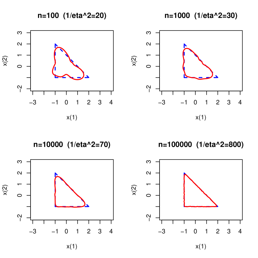
Figure 1: Estimation of triangular shape.

4.2 $l_{1/2}$-spherical shape

We take $r(x)=(|x(1)|^{1/2}+|x(2)|^{1/2})^{2}$, $x=(x(1),x(2))$. Then $Z=\{(x(1),x(2)):|x(1)|^{1/2}+|x(2)|^{1/2}=1\}$ is the unit $l_{1/2}$-sphere. We can calculate $1/c_{0}=\int_{{\mathbb{S}}^{1}}r(u)^{-2}du=4\int_{0}^{\pi/2}\{(\cos\theta)^{1/2}+(\sin\theta)^{1/2}\}^{-4}d\theta=4/3$.

We choose $h(r)\propto\exp(-2r^{1/2})$, so $h(r)=c_{1}\exp(-2r^{1/2})$, say. Then $c_{0}=\int_{0}^{\infty}h(r)rdr=c_{1}\int_{0}^{\infty}\exp(-2r^{1/2})rdr=(3/4)c_{1}$ and hence $c_{1}=(4/3)c_{0}=1$. Thus, our star-shaped distribution is $\exp\{-2r(x)^{1/2}\}dx$.

This star-shaped distribution $\exp\{-2r(x)^{1/2}\}dx$ is obtained as the distribution of $x=(x(1),x(2))$ with $x(1)$ and $x(2)$ being independently distributed according to the $p$-generalized normal distribution with $p=1/2$ (this $p$ does not indicate the dimension of ${\cal X}={\mathbb{R}}^{p}\setminus\{{\bf 0}\}$): $x(j)\sim\exp(-2|x(j)|^{1/2}),\ j=1,2$. We generate $x(j),\ j=1,2$, by using the R package pgnorm.

Our estimator of $Z$ is $\hat{Z}_{n}=\{(2/\sqrt{3})\hat{f}_{n}(u)^{1/2}u:u\in{\mathbb{S}}^{1}\}$.

For visibility, we enlarge the shape and its estimator, and display $10Z$ (blue, dashed line) and $10\hat{Z}_{n}$ (red, solid line) for $n=100,1000,10000,100000$ in Figure 2.

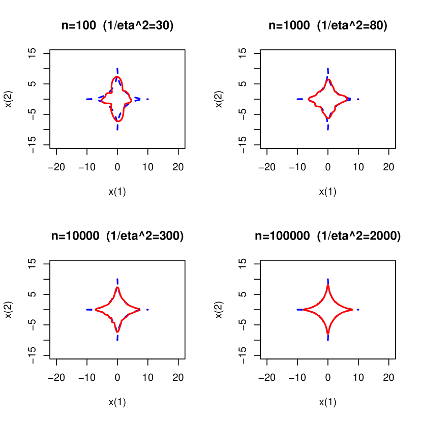
Figure 2: Estimation of $l_{1/2}$-spherical shape.

5 Concluding remarks

In this paper, we proposed a nonparametric estimator of the shape of the density contours of star-shaped distributions, and proved its strong consistency with respect to the Hausdorff distance.

We can introduce the location parameter and consider a star-shaped distribution whose density contours are (unions of) boundaries of star-shaped sets with respect to the location. In that case, one possibility for estimating the shape is to plug in an estimator of the location and use our proposed nonparametric estimator of the shape. We might be able to estimate the location by characterizing it in some way. For example, if the star-shaped distribution may be assumed to be centrally symmetric about the location and have a finite first moment, the location can be characterized as the mean and may be estimated by, e.g., the sample mean. If, instead, $h$ in (1) is strictly decreasing, the location can be regarded as the mode and be estimated by means of various methods for estimating the multivariate mode.

References

- [1] Z. D. Bai, C. R. Rao and L. C. Zhao, Kernel estimators of density function of directional data, Journal of Multivariate Analysis 27 (1988), 24–39.
- [2] K.-T. Fang and Y.-T. Zhang, Generalized Multivariate Analysis, Science Press, Beijing and Springer-Verlag, Berlin, 1990.
- [3] C. Fernández, J. Osiewalski and M. F. J. Steel, Modeling and inference with -spherical distributions, Journal of the American Statistical Association 90 (1995), 1331–1340.
- [4] M. G. Genton (ed.), Skew-Elliptical Distributions and Their Applications: A Journey Beyond Normality, Chapman & Hall/CRC, Boca Raton, 2004.
- [5] P. Hall, G. S. Watson and J. Cabrera, Kernel density estimation with spherical data, Biometrika 74 (1987), 751–762.
- [6] H. Kamiya and A. Takemura, Hierarchical orbital decompositions and extended decomposable distributions, Journal of Multivariate Analysis 99 (2008), 339–357.
- [7] H. Kamiya, A. Takemura and S. Kuriki, Star-shaped distributions and their generalizations, Journal of Statistical Planning and Inference 138 (2008), 3429–3447.
- [8] E. Liebscher and W.-D. Richter, Estimation of star-shaped distributions, Risks 4 (2016), 4: 1–37.
- [9] A. Takemura and S. Kuriki, Theory of cross sectionally contoured distributions and its applications, Discussion Paper Series 96-F-15, July 1996, Faculty of Economics, The University of Tokyo.
- [10] Z. Yang and S. Kotz, Center-similar distributions with applications in multivariate analysis, Statistics Probability Letters 64 (2003), 335–345.