Learning Policies for Markov Decision Processes from Data ††thanks: Submitted for publication. Research partially supported by the NSF under grants CNS-1239021, CCF-1527292, and IIS-1237022, and by the ARO under grants W911NF-11-1-0227 and W911NF-12-1-0390. Hao Liu has been supported by the Lin Guangzhao & the Hu Guozan Graduate Education International Exchange Fund.
Abstract
We consider the problem of learning a policy for a Markov decision process consistent with data captured on the state-actions pairs followed by the policy. We assume that the policy belongs to a class of parameterized policies which are defined using features associated with the state-action pairs. The features are known a priori, however, only an unknown subset of them could be relevant. The policy parameters that correspond to an observed target policy are recovered using -regularized logistic regression that best fits the observed state-action samples. We establish bounds on the difference between the average reward of the estimated and the original policy (regret) in terms of the generalization error and the ergodic coefficient of the underlying Markov chain. To that end, we combine sample complexity theory and sensitivity analysis of the stationary distribution of Markov chains. Our analysis suggests that to achieve regret within order , it suffices to use training sample size on the order of , where is the number of the features. We demonstrate the effectiveness of our method on a synthetic robot navigation example.
1 Introduction
Markov Decision Processes (MDPs) offer a framework for many dynamic optimization problems under uncertainty [1, 2]. When the state-action space is not large and transition probabilities for all state-action pairs are known, standard techniques such as policy iteration and value iteration can compute an optimal policy. More often than not, however, problem instances of realistic size have very large state-action spaces and it becomes impractical to know the transition probabilities everywhere and compute an optimal policy using these off-line methods.
For such large problems, one resorts to approximate methods, collectively referred to as Approximate Dynamic Programming (ADP) [3, 4]. ADP methods approximate either the value function and/or the policy and optimize with respect to the parameters, as for instance is done in actor-critic methods [5, 6, 7]. The optimization of approximation parameters requires the learner to have access to the system and be able to observe the effect of applied control actions.
In this paper, we adopt a different perspective and assume that the learner has no direct access to the system but only has samples of the actions applied in various states of the system. These actions applied in various states are generated according to a policy that is fixed but unknown. As an example, the actions could be followed by an expert player who plays an optimal policy. Our goal is to learn a policy consistent with the observed states-actions, which we will call demonstrations.
Learning from an expert is a problem that has been studied in the literature and referred to as apprenticeship learning [8, 9], imitation learning [10] or learning from demonstrations [11]. While there are many settings where it could be useful, the main application driver has been robotics [12, 13, 14]. Additional interesting application examples include: learning from an experienced human pilot/driver to navigate vehicles autonomously, learning from animals to develop bio-inspired policies, and learning from expert players of a game to train a computer player. In all these examples, and given the size of the state-action space, we will not observe the actions of the expert in all states, or more broadly “scenarios” corresponding to parts of the state space leading to similar actions. Still, our goal is to learn a policy that generalizes well beyond the scenarios that have been observed and is able to select appropriate actions even at unobserved parts of the state space.
A plausible way to obtain such a policy is to learn a mapping of the states-actions to a lower dimensional space. Borrowing from ADP methods, we can obtain a lower-dimensional representation of the state-action space through the use of features that are functions of the state and the action taken at that state. In particular, we will consider policies that combine various features through a weight vector and reduce the problem of learning the policy to learning this weight/parameter vector. Essentially, we will be learning a parsimonious parametrization of the policy used by the expert.
The related work in the literature on learning through demonstrations can be broadly classified into direct and indirect methods [13]. In the direct methods, supervised learning techniques are used to obtain a best estimate of the expert’s behavior; specifically, a best fit to the expert’s behavior is obtained by minimizing an appropriately defined loss function. A key limitation of this method is that the estimated policy is not well adapted to the parts of the state space not visited often by the expert, thus resulting in poor action selection if the system enters these states. Furthermore, the loss function can be non-convex in the policy, rendering the corresponding problem hard to solve.
Indirect methods, on the other hand, evaluate a policy by learning the full description of the MDP. In particular, one solves a so called inverse reinforcement learning problem which assumes that the dynamics of the environment are known but the one-step reward function is unknown. Then, one estimates the reward function that the expert is aiming to maximize through the demonstrations, and obtains the policy simply by solving the MDP. A policy obtained in this fashion tends to generalize better to the states visited infrequently by the expert, compared to policies obtained by direct methods. The main drawback of inverse reinforcement learning is that at each iteration it requires to solve an MDP which is computationally expensive. In addition, the assumption that the dynamics of the environment are known for all states and actions is unrealistic for problems with very large state-action spaces.
In this work, we exploit the benefits of both direct and indirect methods by assuming that the expert is using a Randomized Stationary Policy (RSP). As we alluded to earlier, an RSP is characterized in terms of a vector of features associated with state-action pairs and a parameter weighing the various elements of the feature vector. We consider the case where we have many features, but only relatively few of them are sufficient to approximate the target policy well. However, we do not know in advance which features are relevant; learning them and the associated weights (elements of ) is part of the learning problem.
We will use supervised learning to obtain the best estimate of the expert’s policy. As in actor-critic methods, we use an RSP which is a parameterized “Boltzmann” policy and rely on an -regularized maximum likelihood estimator of the policy parameter vector. An -norm regularization induces sparse estimates and this is useful in obtaining an RSP which uses only the relevant features. In [15], it is shown that the sample complexity of -penalized logistic regression grows as , where is the number of features. As a result, we can learn the parameter vector of the target RSP with relatively few samples, and the RSP we learn generalizes well across states that are not included in the demonstrations of the expert. Furthermore, -regularized logistic regression is a convex optimization problem which can be solved efficiently.
1.1 Related Work
There is substantial work in the literature on learning MDP policies by observing experts; see [13] for a survey. We next discuss papers that are more closely related to our work.
In the context of indirect methods, [16] develops techniques for estimating a reward function from demonstrations under varying degrees of generality on the availability of an explicit model. [8] introduces an inverse reinforcement learning algorithm that obtains a policy from observed MDP trajectories followed by an expert. The policy is guaranteed to perform as well as that of the expert’s policy, even though the algorithm does not necessarily recover the expert’s reward function. In [9], the authors combine supervised learning and inverse reinforcement learning by fitting a policy to empirical estimates of the expert demonstrations over a space of policies that are optimal for a set of parameterized reward functions. [9] shows that the policy obtained generalizes well over the entire state space. [11] uses a supervised learning method to learn an optimal policy by leveraging the structure of the MDP, utilizing a kernel-based approach. Finally, [10] develops the DAGGER (Dataset Aggregation) algorithm that trains a deterministic policy which achieves good performance guarantees under its induced distribution of states.
Our work is different in that we focus on a parameterized set of policies rather than parameterized rewards. In this regard, our work is similar to approximate DP methods which parameterize the policy, e.g., expressing the policy as a linear functional in a lower dimensional parameter space. This lower-dimensional representation is critical in overcoming the well known “curse of dimensionality.”
1.2 Contributions
We adopt the -regularized logistic regression to estimate a target RSP that generates a given collection of state-action samples. We evaluate the performance of the estimated policy and derive a bound on the difference between the average reward of the estimated RSP and the target RSP, typically referred to as regret. We show that a good estimation of the parameter of the target RSP also implies a good bound on the regret. To that end, we generalize a sample complexity result on the log-loss of the maximum likelihood estimates [15] from the case of two actions available at each state to the multi-action case. Using this result, we establish a sample complexity result on the regret.
Our analysis is based on the novel idea of separating the loss in average reward into two parts. The first part is due to the error in the policy estimation (training error) and the second part is due to the perturbation in the stationary distribution of the Markov chain caused by using the estimated policy instead of the true target policy (perturbation error). We bound the first part by relating the result on the log-loss error to the Kulback-Leibler divergence [17] between the estimated and the target RSPs. The second part is bounded using the ergodic coefficient of the induced Markov chain. Finally, we evaluate the performance of our method on a synthetic example.
The paper is organized as follows. In Section 2, we introduce some of our notation and state the problem. In Section 3, we describe the supervised learning algorithm used to train the policy. In Section 4, we establish a result on the (log-loss) error in policy estimation. In Section 5, we establish our main result which is a bound on the regret of the estimated policy. In Section 7, we introduce a robot navigation example and present our numerical results. We end with concluding remarks in Section 8.
Notational conventions. Bold letters are used to denote vectors and matrices; typically vectors are lower case and matrices upper case. Vectors are column vectors, unless explicitly stated otherwise. Prime denotes transpose. For the column vector we write for economy of space, while denotes its -norm. Vectors or matrices with all zeroes are written as , the identity matrix as , and is the vector with all entries set to . For any set , denotes its cardinality. We use to denote the natural logarithm and a subscript to denote different bases, e.g., denotes logarithm with base .
2 Problem Formulation
Let denote a Markov Decision Process (MDP) with a finite set of states and a finite set of actions . For a state-action pair , let denote the probability of transitioning to state after taking action in state . The function denotes the one-step reward function.
Let us now define a class of Randomized Stationary Policies (RSPs) parameterized by vectors . Let denote the set of RSPs we are considering. For a given parameter and a state , denotes the probability of taking action at state . Specifically, we consider the Boltzmann-type RSPs of the form
| (1) |
where is a vector of features associated with each state-action pair . (Features are normalized to take values in .) Henceforth, we identify an RSP by its parameter . We assume that the policy is sparse, that is, the vector has only non-zero components and each is bounded by , i.e., for all . Given an RSP , the resulting transition probability matrix on the Markov chain is denoted by , whose element is for all state pairs .
Notice that for any RSP , the sequence of states and the sequence of state-action pairs form a Markov chain with state space and , respectively. We assume that for every , the Markov chains and are irreducible and aperiodic with stationary probabilities and , respectively.
The average reward function associated with an RSP is a function defined as
| (2) |
Let now fix a target RSP . As we assumed above, is sparse having at most non-zero components , each satisfying . This is simply the policy used by an expert (not necessarily optimal) which we wish to learn. We let denote a set of state-action samples generated by playing policy . The state samples are independent and identically distributed (i.i.d.) drawn from the stationary distribution and is the action taken in state according to the policy . It follows that the samples in are i.i.d. according to the distribution .
We assume we have access only to the demonstrations while the transition probability matrix and the target RSP are unknown. The goal is to learn the target policy and characterize the average reward obtained when the learned RSP is applied to the Markov process. In particular, we are interested in estimating the target parameter from the samples efficiently and evaluate the performance of the estimated RSP with respect to the target RSP, i.e., bound the regret defined as
where is the estimated RSP from the samples .
3 Estimating the policy
Next we discuss how to estimate the target RSP from the i.i.d. state-action training samples in . Given the Boltzmann structure of the RSP we have assumed, we fit a logistic regression function using a regularized maximum likelihood estimator as follows:
| (3) |
where is a parameter that adjusts the trade-off between fitting the training data “well” and obtaining a sparse RSP that generalizes well on a test sample.
We can evaluate how well the maximum likelihood function fits the samples in the logistic function using a log-loss metric, defined as the expected negative of the likelihood over the (random) test data. Formally, for any parameter , log-loss is given by
| (4) |
where the expectation is taken over state-action pairs drawn from the distribution ; recall that we defined to be the stationary distribution of the state-action pairs induced by the policy . Since the expectation is taken with respect to new data not included in the training set , we can think of as an out-of-sample metric of how well the RSP approximates the actions taken by the target RSP .
We also define a sample-average version of log-loss: given any set of state-action pairs, define
| (5) |
We will use the term empirical log-loss to refer to log-loss over the training set and use the notation
| (6) |
To estimate an RSP, say , from the training set, we adopt the logistic regression with regularization introduced in [15]. The specific steps are shown in Algorithm 1.
4 Log-loss performance
In this section we establish a sample complexity result indicating that relatively few training samples (logarithmic in the dimension of the RSP parameter ) are needed to guarantee that the estimated RSP has out-of-sample log-loss close to the target RSP . We will use the line of analysis in [15] but generalize the result from the case where only two actions are available for every state to the general multi-action setting.
We start by relating the difference of the log-loss function associated with RSP and its estimate to the relative entropy, or Kullback-Leibler (KL) divergence, between the corresponding RSPs. For a given , we denote the KL-divergence between RSPs, and as , where denotes the probability distribution induced by RSP on in state , and is given as follows:
We also define the average KL-divergence, denoted by , as the average of over states visited according to the stationary distribution of the Markov chain induced by policy . Specifically, we define
Lemma 4.1
Let be an estimate of RSP . Then,
Proof:
∎
For the case of a binary action at every state, [15] showed the following result. To state the theorem, let denote a function which is polynomial in its arguments and recall that is the number of state-action pairs in the training set used to learn .
Theorem 4.2 ([15], Thm. 3.1)
Suppose action set contains only two actions, i.e. . Let and . In order to guarantee that, with probability at least , produced by the algorithm performs as well as , i.e.,
it suffices that .
We will generalize the result to the case when more than two actions are available at each state. We assume that , that is, at most actions are available at each state. By introducing in (1) features that get activated at specific states, it is possible to accommodate MDPs where some of the actions are not available at these states.
Theorem 4.3
Let and . In order to guarantee that, with probability at least , produced by Algorithm 1 performs as well as , i.e.,
| (7) |
it suffices that
Furthermore, in terms of only , .
The remainder of this section is devoted to proving Theorem 4.3. The proof is similar to the proof of Theorem 4.2 (Theorem 3.1 in [15]) but with key differences to accommodate the multiple actions per state. We start by introducing some notations and stating necessary lemmata.
Denote by a class of functions over some domain and range . Let , which is the valuation of the class of functions at a certain collection of points . It is said that a set of vectors in -covers in the -norm, if for every point there exists some , , such that . Let also denote the size of the smallest set that -covers in the -norm. Finally, let
To simplify the representation of log-loss of the general logistic function in (1), we use the following notations. For each , denotes feature vectors associated with each action. For any , define the -likelihood function as
Note . Further, let be the class of functions . We can then rewrite using as .
Lemma 4.5 ([19])
Suppose and the input has a norm-bound such that , where . Then
| (8) |
Lemma 4.7
Let be a class of functions from to some bounded set in . Consider as a class of functions from to some bounded set in , with the following form:
| (9) |
If is Lipschitz with Lipschitz constant in the -norm for every , then we have
Proof: Let . It is sufficient to show for every inputs
we can find points in that -cover . Fix some set of points . From the definition of , for each ,
Let 111One may find less than points, but we consider the worst case scenario. be a set of points in that -covers . We use notation to denote the th element of vector . Then, for any and , there exists a such that
| (10) |
Now consider points with the following form
where .
Given a and , let be as defined above and consider
where we used the Lipschitz property of the function in the first inequality and the last inequality follows from (4). Thus, the points -cover in -norm. Finally, notice that the set of points is arbitrary, which concludes the proof. ∎
We now continue with the proof of Theorem 4.3. Recall Algorithm 1 and let be the smallest integer in that is greater or equal to . Notice that in Algorithm 1 one can use a larger but we select the smallest possible to obtain a tighter bound. For such a , it follows that . Define a class of functions with domain as
The partial derivatives of the log-loss function are
and it can be seen that
Hence, the Lipschitz constant for is for any .
We next find the range of class . To begin with, the range of class is
Since is Lipschitz in -norm with Lipschitz constant and (by the fact ), then
which implies
| (12) |
Finally, let , which is the size of training set in Algorithm 1. From Lemma 4.4, Eq. (12) and Eq. (11), we have
| (13) |
Treat as a constant. To upper bound the right hand side of the above equation by , it suffices to have
| (14) |
The rest of the proof follows closely the proof of Theorem 3.1 in [15]. We outline the key steps for the sake of completeness. Suppose satisfies (14); then, with probability at least , for all
Thus, using our definition of in (9), for any with and with probability at least , we have
Therefore, for all with and with probability at least , it holds
where is the training set from Algorithm 1.
Essentially, we have shown that for large enough the empirical log-loss function is a good estimate of the log-loss function . According to Step 2 of Algorithm 1, . By Lemma 4.6, we have
| (15) |
where is the target policy and the last inequality follows simply from the fact that .
Eq. 15 indicates that the training step of Algorithm 1, finds at least one parameter vector whose performance is nearly as good as that of . At the validation step, we select one of the found during training. It can be shown ([20]) that with a validation set of the same order of magnitude as the training set (and independent of ), we can ensure that with probability at least , the selected parameter vector will have performance at most worse than that of the best performing vector discovered in the training step. Hence, with probability at least , the output of our algorithm satisfies
| (16) |
Finally, replacing with and with everywhere in the proof, establishes Theorem 4.3.
5 Bounds on Regret
Theorem 4.3 provides a sufficient condition on the number of samples required to learn a policy whose log-loss performance is close to the target policy. In this section we study the regret of the estimated policy, defined in Sec. 2 as the difference between the average reward of the target policy and the estimated policy. Given that we use a number of samples in the training set proportional to the expression provided in Theorem 4.3, we establish explicit bounds on the regret.
We will bound the regret of the estimated policy by separating the effect of the error in estimating the policy function (which is characterized by Theorem 4.3) and the effect the estimated policy function introduces in the stationary distribution of the Markov chain governing how states are visited. To bound the regret due to the perturbation of the stationary distribution, we will use results from the sensitivity analysis of Markov chains. In Section 5.1 we provide some standard definitions for Markov chains and state our result on the regret, while in Section 6 we provide a proof of this result.
5.1 Main Result
We start by defining the fundamental matrix of a Markov chain.
Definition 1
The fundamental matrix of a Markov chain with state transition probability matrix induced by RSP is
where denotes the vector of all ’s, and denotes the stationary distribution associated with . Also, the group inverse of denoted as is the unique matrix satisfying
Most of the properties of a Markov chain can be expressed in terms of the fundamental matrix . For example, if is the stationary probability distribution associated with a Markov chain whose transition probability matrix is and if for some perturbation matrix , then the stationary probability distribution of the Markov chain with transition probability matrix satisfies the relation
| (17) |
where is the fundamental matrix associated with .
Definition 2
The ergodic coefficient of a matrix with equal row sums is
| (18) |
The ergodic coefficient of a Markov chain indicates sensitivity of its stationary distribution. For any stochastic matrix , .
We now have all the ingredients to state our main result bounding regret.
Theorem 5.1
Given and , suppose
i.i.d. samples are used by Algorithm 1 to produce an estimate the unknown target RSP policy parameter . Then with probability at least , we have
where
and is a constant that depends on the RSP and can be any of the following:
-
•
,
-
•
,
-
•
,
-
•
.
The constant is referred to as condition number. The regret is thus governed by the condition number of the estimated RSP; the smaller the condition number of the trained policy, the smaller is the regret.
6 Proof of the Main Result
In this section we analyze the average reward obtained by the MDP when we apply the estimated RSP , and prove the regret bound in Theorem 5.1. First, we bound the regret as the sum of two parts.
| (19) | |||||
Note that the first absolute sum above has terms for all that are related to the estimation error from fitting the RSP policy to . The second part has terms that are related to the perturbation of the stationary distribution of the Markov chain by applying the fitted RSP instead of the original . In the following, we bound each term separately. We begin with the first term.
| (20) | |||||
where denotes the probability distribution (a vector) on the action space induced by the RSP at state .
The bound in (20) is related to the difference in the log-loss between the RSPs and . To see this, we need the following result that connects the distance between two distributions with their KL-divergence. Let and denote two probability vectors on . From the variation distance characterization of and we have the following lemma.
Lemma 6.1
([17, Lemma 11.6.1])
| (21) |
Continuing the chain of inequalities from (20), we obtain
| (22) | |||||
In the first inequality, we applied Lemma 6.1 by setting and for each . In second inequality, we applied Jensen’s inequality. We can now use Theorem 4.3 to bound (22).
We next bound the second term in (19) using techniques from perturbation analysis of eigenvalues of a matrix. We have
| (23) | |||||
where we used the definition of in the 2nd inequality and the last equality follows by noting that for all . To further bound the difference in stationary distributions in (23), we use a relation between a measure of perturbation of the stationary distribution and the condition number of Markov chains. We recall the following result that is useful to bound the difference between the stationary distribution induced by the optimal RSP and that induced by the estimated RSP in terms of the condition number of the Markov chains.
Lemma 6.2 ([21, 22])
Let and be the unique stationary distributions of the stochastic matrices and , respectively. Let . Then,
| (24) |
where is a constant that can take the following values
-
•
,
-
•
,
-
•
,
-
•
.
Proof: The proof follows by setting and in (17) and using the relation
The other relations follow similarly from Sec. 3 of [22]. ∎
Continuing the chain of inequalities in (23) and applying Lemma 6.2 by setting and , we obtain
| (25) |
where, with some overloading of notation, is now as specified in the expressions provided in the statement of Theorem 5.1.
The th component of the vector is given by
where, in the last equality, we applied the definition of the transition probability associated with RSP .
It follows
| (26) |
where the last inequality follows by noting that for all .
7 A robot navigation example
In this section, we discuss the experimental setup to simulate an MDP and validate the effectiveness of our proposed learning algorithm. We consider the problem of learning the policy used by an agent (a robot) as it moves on a 2-dimensional grid. After simulating the movement of the robot and recording its actions in various states, we use these states-action samples to learn the policy of the robot and evaluate its performance.
7.1 Environment and Agent Settings
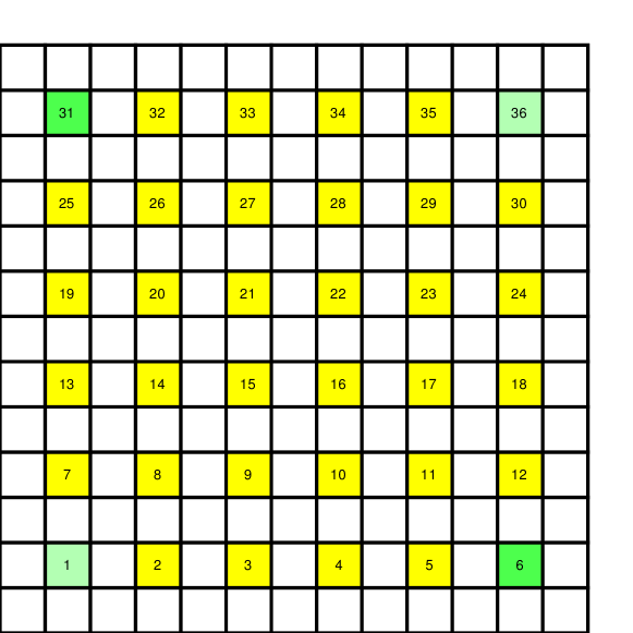
Consider an agent moving in a grid, shown in Fig. 1. The agent’s position is specified by a two-tuple state , representing its coordinates in the grid. We assume is at the southwest corner of the grid and we make the convention that coordinates on the grid identify the square defined by the four points , , , and . For example, when we say that the agent is at we mean that the agent can be anywhere in the above square.
At each time instance, the agent can take actions: North, East, West, and South. Without loss of generality, we assume that the agent can only move to a neighboring grid point. The destination of the agent is based on its current position and the action. We assume that the agent movements are subject to uncertainty, which can cause the agent’s intended next position to shift to a point adjacent to that position. For example, the agent in state taking action North will enter state with probability (the intended next position), but can enter states or with probability , respectively. At the boundary points of the grid, the agent bounces against the “wall” in the opposite direction with its position unchanged.
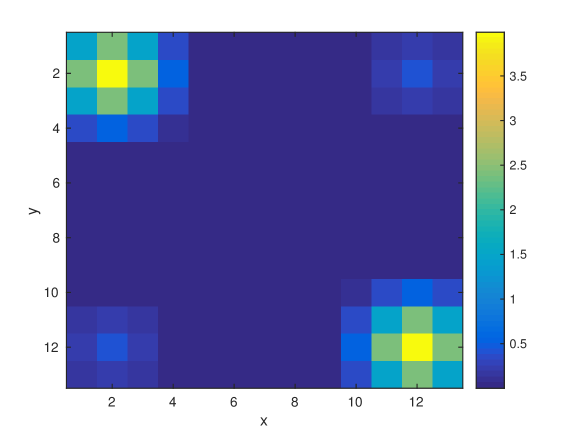
The environment contains points with associated rewards. Specifically, as showed in Fig. 1, squares (waypoints) labeled and have associated reward equal to and squares (waypoints) labeled and have associated reward equal to . The reward of a waypoint “spreads” on the grid according to a Gaussian function. Specifically, the immediate reward at point due to the reward waypoint is given by
and is constant for all actions. Summing over all reward waypoints , the immediate reward at some point is given by
| (28) |
where we assume that a point with no associated reward satisfies . The one step reward function induced by the four reward waypoints of Fig. 1 is shown in Fig. 2.
The agent (robot) entering some state (position) collects reward equal to the immediate reward . The objective of the agent is to navigate on the grid so as to maximize the long-term average reward collected.
The key step of efficient learning is to define appropriate features we will use to represent the agent’s policy. The way of selecting features in this paper is inspired by spline interpolation [23]. We define waypoints on the grid, shown in Fig. 1. For a state-action pair , we set to be the intended next state and define the features
where is as defined as
and is the location of the th waypoint.
7.2 Simulation and Learning Performance
For the MDP we have introduced, we use value iteration [2] to find the best policy. We generate independent state-action samples according to this policy. Then, we estimate the policy using the above samples according to the logistic regression algorithm discussed in Section 3. We largely follow the style of [15] in presenting our numerical results. We compare average rewards from different policies with respect to the number of features and the number of samples as follows:
-
1.
Target policy: We choose the policy obtained by the value iteration algorithm [2] as the target policy. It is used to generate samples for learning.
-
2.
-regularized policy: The RSP trained using the Algorithm in Section 3.
- 3.
-
4.
Greedy policy: The agent takes the action with the largest expected next step reward, i.e., the local reward feature is the only consideration. This policy is used as a baseline.
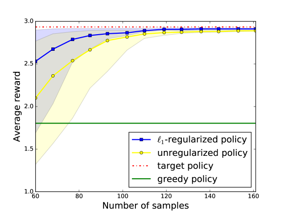
We randomly sample the state-action pairs generated by the optimal policy and use these samples to form a training set to be used in learning an RSP (as in Section 3). This process is repeated times. The average rewards of all policies we considered as a function of the number of samples used for training are displayed in Fig. 3. As shown in Fig. 3, the -regularized policy performs closely to the target policy, even with a very small number of training samples. Not surprisingly, both the -regularized and the unregularized policy perform almost as well as the optimal policy when the number of training samples grows large. For most runs, the policies we learn (both regularized and unregularized) perform better than the greedy policy.
It is interesting that when the number of samples is small, the regularized policy performs better. This is because the unregularized policy tends to overfit to the training samples while the regularized policy seeks to learn fewer parameters and thus ends up learning them better, in a way that generalizes well out-of-sample. In sum, this simulation example supports the effectiveness of our algorithm.
.
8 Conclusion
We considered the problem of learning a policy in a Markov decision process using the state-action samples associated with the policy. We focused on a Boltzmann-type policy that is characterized by feature vectors associated with each state-action pair and a parameter that is sparse.
To learn the policy, we used -regularized logistic regression and showed that a good generalization error bound also guarantees a good bound on the regret, defined as the difference between the average reward of the estimated policy and the target policy. Our results suggest that one can estimate an effective policy using a training set of size proportional to the logarithm of the number of features used to represent the policy.
References
- [1] M. Puterman, Markov Decision Processes: Discrete Stochastic Dynamic Programming. John Wiley & Sons, Inc. New York, NY, USA, 1994.
- [2] D. P. Bertsekas, Dynamic Programming and Optimal Control. Belmont, MA: Athena Scientific, 1995, vol. I and II.
- [3] D. Bertsekas and J. Tsitsiklis, Neuro-Dynamic Programming. Belmont, MA: Athena Scientific, 1996.
- [4] W. Powell, Approximate Dynamic Programming. John Wiley and Sons, 2007.
- [5] V. R. Konda and J. N. Tsitsiklis, “Actor-critic algorithms,” SIAM Journal on Control and Optimization, vol. 42, no. 4, pp. 1143–1166, 2003.
- [6] J. Wang and I. C. Paschalidis, “An actor-critic algorithm with second-order actor and critic,” IEEE Trans. Automat. Contr., 2016, in print.
- [7] R. Moazzez-Estanjini, K. Li, and I. C. Paschalidis, “A least squares temporal difference actor-critic algorithm with applications to warehouse management,” Naval Research Logistics, vol. 59, no. 3, pp. 197–211, 2012.
- [8] P. Abbeel and A. Y. Ng, “Apprenticeship learning vis inverse reinforcement leaning,” in Proceedings of the International Conference on Machine Learning (ICML), 2004.
- [9] G. Neu and S. Szepesvari, “Apprenticeship learning using inverse reinforcement learning and gradient methods,” in Proceedings of the Uncertainty in Artificial Intelligence (UAI), 2007.
- [10] S. Ross, G. J. Gordon, and J. A. Bagnell, “A reduction of imitation learning and structured prediction to no-regret online learning,” in Proceedings of the Artificial Intelligence and Statistics (AISTATS), 2011.
- [11] F. S. Melo and M. Lopes, “Learning from demonstration using MDP induced matrics,” in Proceedings of the European Conference on Machine Learning (ECML), 2010.
- [12] S. Schaal, “Is imitation learning the route to humanoid robots?” in In Trends in Cognitive Sciences, 1999.
- [13] B. Argall, S. Chernova, and M. Veloso, “A survey of robot learning from demonstrations,” Robotics and Autonomous System, vol. 57, no. 5, 2009.
- [14] W. Erlhagen, A. Mukovskiy, E. Bicho, G. Panin, C. Kiss, A. Knoll, H. Van Schie, and H. Bekkering, “Goal-directed imitation for robots: A bio-inspired approach to action understanding and skill learning,” Robotics and autonomous systems, vol. 54, no. 5, pp. 353–360, 2006.
- [15] A. Y. Ng, “Feature selection, vs. regularization, and rotational invariance,” in Proceedings of the International Conference on Machine Learning (ICML), June 2004.
- [16] A. Y. Ng and S. Russell, “Algorithms for inverse reinforcement learning,” in Proceedings of the International Conference on Machine Learning (ICML), 2000.
- [17] T. A. Cover and J. A. Thomas, Elements of Information Theory. John Wiley & Sons, 2006.
- [18] D. Pollard, Convergence of stochastic processes. Springer-Verlag, 1984.
- [19] T. Zhang, “Covering Number Bounds of Certain Regularized Linear Function Classes,” Journal of Machine Learning Research, vol. 2, pp. 527–550, 2002.
- [20] M. Anthony and P. L. Bartlett, Neural network learning: Theoretical foundations. Cambridge University Press, 2009.
- [21] E. Seneta, “Perturbation of the stationary distribution measured by ergodicity coefficients,” Advances in Applied Probability, vol. 20, no. 1, 1998.
- [22] G. E. Cho and C. Meyer, “Comparison of perturbation bounds for the stationary distributions of a Markov chain,” Elsevier journal of Linear Algebra and Its Application, vol. 335, pp. 137–150, 2001.
- [23] C. De Boor, A practical guide to splines. Springer, 1978, vol. 27.