The biglasso Package: A Memory- and Computation-Efficient Solver for Lasso Model Fitting with Big Data in R

Yaohui Zeng, Patrick Breheny biglasso Package biglasso: A Memory- and Computation-Efficient R package for Lasso Penalized regression models such as the lasso have been extensively applied to analyzing high-dimensional data sets. However, due to memory limitations, existing R packages like glmnet and ncvreg are not capable of fitting lasso-type models for ultrahigh-dimensional, multi-gigabyte data sets that are increasingly seen in many areas such as genetics, genomics, biomedical imaging, and high-frequency finance. In this research, we implement an R package called biglasso that tackles this challenge. biglasso utilizes memory-mapped files to store the massive data on the disk, only reading data into memory when necessary during model fitting, and is thus able to handle out-of-core computation seamlessly. Moreover, it’s equipped with newly proposed, more efficient feature screening rules, which substantially accelerate the computation. Benchmarking experiments show that our biglasso package, as compared to existing popular ones like glmnet, is much more memory- and computation-efficient. We further analyze a 31 GB real data set on a laptop with only 16 GB RAM to demonstrate the out-of-core computation capability of biglasso in analyzing massive data sets that cannot be accommodated by existing R packages. lasso, big data, memory-mapping, out-of-core, feature screening, parallel computing, OpenMP, C++ lasso, big data, memory-mapping, out-of-core, hybrid safe-strong rules, parallel computing, C++ Yaohui Zeng
Department of Biostatistics
University of Iowa
N301 CPHB 145 North Riverside Drive
Iowa City, IA 52242, United States of America
Email:
Patrick Breheny
Department of Biostatistics
University of Iowa
N336 CPHB 145 North Riverside Drive
Iowa City, IA 52242, United States of America
E-mail:
URL: http://myweb.uiowa.edu/pbreheny/index.html

1 Introduction

The lasso model proposed by Tibshirani (1996) has fundamentally reshaped the landscape of high-dimensional statistical research. Since its original proposal, the lasso has attracted extensive studies with a wide range of applications to many areas, such as signal processing (Angelosante and Giannakis, 2009), gene expression data analysis (Huang and Pan, 2003), face recognition (Wright et al., 2009), text mining (Li et al., 2015) and so on. The great success of the lasso has made it one of the most popular tools in statistical and machine-learning practice.

Recent years have seen the evolving era of Big Data where ultrahigh-dimensional, large-scale data sets are increasingly seen in many areas such as genetics, genomics, biomedical imaging, social media analysis, and high-frequency finance (Fan et al., 2014). Such data sets pose a challenge to solving the lasso efficiently in general, and for R specifically, since R is not naturally well-suited for analyzing large-scale data sets (Kane et al., 2013). Thus, there is a clear need for scalable software for fitting lasso-type models designed to meet the needs of big data.

In this project, we develop an R package, biglasso (Zeng and Breheny, 2016), to extend lasso model fitting to Big Data in R. Specifically, sparse linear and logistic regression models with lasso and elastic net penalties are implemented. The most notable features of biglasso include:

• It utilizes memory-mapped files to store the massive data on the disk, only loading data into memory when necessary during model fitting. Consequently, it’s able to seamlessly handle out-of-core computation.

• It is built upon pathwise coordinate descent algorithm and “warm start” strategy, which has been proven to be one of fastest approaches to solving the lasso (Friedman et al., 2010).

• We develop new, hybrid feature screening rules that outperform state-of-the-art screening rules such as the sequential strong rule (SSR) (Tibshirani et al., 2012), and the sequential EDPP rule (SEDPP) (Wang et al., 2015) with additional 1.5x to 4x speedup.

• The implementation is designed to be as memory-efficient as possible by eliminating extra copies of the data created by other R packages, making biglasso at least 2x more memory-efficient than glmnet.

• The underlying computation is implemented in C++, and parallel computing with OpenMP is also supported.

The methodological innovation and well-designed implementation have made biglasso a much more memory- and computation-efficient and highly scalable lasso solver, as compared to existing popular R packages like glmnet (Friedman et al., 2010), ncvreg (Breheny and Huang, 2011), and picasso (Ge et al., 2015). More importantly, to the best of our knowledge, biglasso is the first R package that enables the user to fit lasso models with data sets that are larger than available RAM, thus allowing for powerful big data analysis on an ordinary laptop.

The rest of the paper is organized as follows. In Section 2, we describe the memory-mapping technique for out-of-core computation as well as our newly developed hybrid safe-strong rule for feature screening. In Section 3, we discuss some important implementation techniques as well as parallel computation that make biglasso memory- and computation-efficient. Section 4 presents benchmarking experiments with both simulated and real data sets. Section 5 provides a brief, reproducible demonstration illustrating how to use biglasso, while 6 demonstrates the out-of-core computation capability of biglasso through its application to a large-scale genome-wide association study. We conclude the paper with some final discussions in Section 7.

2 Method

2.1 Memory mapping

Memory mapping (Bovet and Cesati, 2005) is a technique that maps a data file into the virtual memory space so that the data on the disk can be accessed as if they were in the main memory. Technically, when the program starts, the operating system (OS) will cache the data into RAM. Once the data are in RAM, the computation is at the standard in-memory speed. If the program requests more data after the memory is fully occupied, which is inevitable in the data-larger-than-RAM case, the OS will move data that is not currently needed out of RAM to create space for loading in new data. This is called the page-in-page-out procedure, and is automatically handled by the OS.

The memory mapping technique is commonly used in modern operating systems such as Windows and Unix-like systems due to several advantages:

1. it provides faster file read/write than traditional I/O methods since data-copy from kernel to user buffer is not needed due to page caches;

2. it allows random access to the data as if it were in the main memory even though it physically resides on the disk;

3. it supports concurrent sharing in that multiple processes can access the same memory-mapped data file simultaneously, making parallel computing easy to implement in data-larger-than-RAM cases;

4. it enables out-of-core computing thanks to the automatic page-in-page-out procedure.

We refer the readers to Rao et al. (2010), Lin et al. (2014), and Bovet and Cesati (2005) for detailed techniques and some successful applications of memory mapping.

To take advantage of memory mapping, biglasso creates memory-mapped big matrix objects based upon the R package bigmemory (Kane et al., 2013), which uses the Boost C++ library and implements memory-mapped big matrix objects that can be directly used in R. Then at the C++ level, biglasso uses the C++ library of bigmemory for underlying computation and model fitting.

2.2 Efficient feature screening

Another important contribution of biglasso is our newly developed hybrid safe-strong rule, named SSR-BEDPP, which substantially outperforms existing state-of-the-art ones in terms of the overall computing time of obtaining the lasso solution path. Here, we describe the main idea of hybrid rules; for the technical details, see Zeng et al. (2017).

Feature screening aims to identify and discard inactive features (i.e., those with zero coefficients) from the lasso optimization. It often leads to dramatic dimension reduction and hence significant computation savings. However, these savings will be negated if the screening rule itself is too complicated to execute. Therefore, an efficient screening rule needs to be powerful enough to discard a large portion of features and also relatively simple to compute.

Existing screening rules for the lasso can be divided into two types: (1) heuristic rules, such as the sequential strong rule (SSR) (Tibshirani et al., 2012), and (2) safe rules, such as the basic and the sequential EDPP rules (Wang et al., 2015), denoted here as BEDPP and SEDPP respectively. Safe rules, unlike heuristic ones, are guaranteed to never incorrectly screen a feature with a nonzero coefficient. Figure 1 compares the power of the three rules in discarding features. SSR, though most powerful among the three, requires a cumbersome post-convergence check to verify that it has not incorrectly discarded an active feature. The SEDPP rule is both safe and powerful, but is inherently complicated and time-consuming to evaluate. Finally, BEDPP is the least powerful, and discards virtually no features when $\lambda$ is smaller than 0.45 (in this case), but is both safe and involves minimal computational burden.

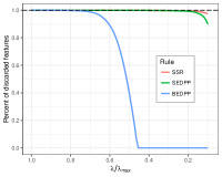
Figure 1: Percent of features discarded.

The rule employed by biglasso, SSR-BEDPP, as its name indicates, combines SSR with the simple yet safe BEDPP rule. The rationale is to alleviate the burden of post-convergence checking for strong rules by not checking features that can be safely eliminated using BEDPP. This hybrid approach leverages the advantages of each rule, and offers substantial gains in efficiency, especially when solving the lasso for large values of $\lambda$.

Table 1 summarizes the complexities of the four rules when applied to solving the lasso along a path of $K$ values of $\lambda$ for a data set with $n$ instances and $p$ features. SSR-BEDPP can be substantially faster than the other three rules when BEDPP is effective. Furthermore, it is important to note that SSR (with post-convergence checking) and SEDPP have to scan the entire feature matrix at every value of $\lambda$, while SSR-BEDPP only needs to scan the features not discarded by BEDPP. This advantage of SSR-BEDPP is particularly appealing in out-of-core computing, where fully scanning the feature matrix requires disk access and therefore becomes the computational bottleneck of the procedure.

Rule	Complexity
SSR	$O(npK)$
SEDPP	$O(npK)$
BEDPP	$O(np)$
SSR-BEDPP	$O(n\sum_{k}^{K}|\mathcal{S}_{k}|))$

Table 1: Complexity of computing screening rules along the entire path of $K$ values of $\lambda$. $|\mathcal{S}_{k}|$ denotes the cardinality of $\mathcal{S}_{k}$, the safe set of features not discarded by BEDPP screening.

The hybrid screening idea is straightforward to extend to other lasso-type problems provided that a corresponding safe rule exists. For the biglasso package, we also implemented a hybrid screening rule, SSR-Slores, for lasso-penalized logistic regression by combining SSR with the so-called Slores rule (Wang et al., 2014), a safe screening rule developed for sparse logistic regression.

3 Implementation

3.1 Memory-efficient design

In penalized regression models, the feature matrix $\mathbf{X}\in\mathbb{R}^{n\times p}$ is typically standardized to ensure that the penalty is applied uniformly across features with different scales of measurement. In addition, standardization contributes to faster convergence of the optimization algorithm. In existing R packages such as glmnet, ncvreg, and picasso, a standardized feature matrix $\widetilde{\mathbf{X}}$ is calculated and stored, effectively doubling memory usage. This problem is compounded by cross-validation, where these packages also calculate and store additional standardized and unstandardized copies of $\mathbf{X}$ for each fold. This approach does not scale up well for big data.

To make the memory usage more efficient, biglasso doesn’t store $\widetilde{\mathbf{X}}$. Instead, it saves only the means and standard deviations of the columns of $\mathbf{X}$ as two vectors, denoted as $\mathbf{c}$ and $\mathbf{s}$. Then wherever $\widetilde{x}_{ij}$ is needed, it is retrieved by “cell-wise standardization”, i.e., $\widetilde{x}_{ij}=(x_{ij}-c_{j})/s_{j}$. Additionally, the estimated coefficient matrix is sparse-coded in C++ and R to save memory space.

3.1.1 Simplification of computations

Cell-wise standardization saves a great deal of memory space, but at the expense of computational efficiency. To minimize this, biglasso uses a number of computational strategies to eliminate redundant calculations.

We first note that the computations related to $\widetilde{\mathbf{X}}$ during whole model fitting process are mainly of three types, and all can be simplified so that naïve cell-wise standardization can be avoided:

1. $\widetilde{\mathbf{x}}_{j}^{T}\widetilde{\mathbf{x}}_{*}=\sum_{i}\frac{x_{ij}-c_{j}}{s_{j}}\frac{x_{i*}-c_{*}}{s_{*}}=\frac{1}{s_{j}s_{*}}\big{(}\sum_{i}x_{ij}x_{i*}-nc_{j}c_{*}\big{)}$;

2. $\widetilde{\mathbf{x}}_{i}^{T}\mathbf{y}=\sum_{i}\frac{x_{ij}-c_{j}}{s_{j}}y_{i}=\frac{1}{s_{j}}\big{(}\sum_{i}x_{ij}y_{i}-c_{j}\sum_{i}y_{i}\big{)}$;

3. $\widetilde{\mathbf{x}}_{j}^{T}\mathbf{r}=\sum_{i}\frac{x_{ij}-c_{j}}{s_{j}}r_{i}=\frac{1}{s_{j}}\big{(}\sum_{i}x_{ij}r_{i}-c_{j}\sum_{i}r_{i}\big{)}$;

where $\widetilde{\mathbf{x}}_{j}$ is the $j$th column of $\widetilde{\mathbf{X}}$, $\widetilde{\mathbf{x}}_{*}$ is the column corresponding to $\lambda_{\max}$, $\mathbf{y}$ is the response vector, and $\mathbf{r}\in\mathbb{R}^{n}$ is current residual vector.

Type (1) and (2) are used only for initial feature screening, and require only one-time execution. Type (3) occurs in both the coordinate descent algorithm and the post-convergence checking. Since the coordinate descent algorithm is fast to converge and only iterates over features in the active set $\mathcal{A}$ of nonzero coefficients, whose size is much smaller than $p$, the number of additional computations this introduces is small. Moreover, we pre-compute and store $\sum_{i}r_{i}$, which saves a great deal of computation during post-convergence checking since $\mathbf{r}$ does not change during this step. As a result, our implementation of cell-wise standardization requires only $O(p)$ additional operations compared to storing the entire standardized matrix.

3.1.2 Scalable cross-validation

Cross-validation is integral to lasso modeling in practice, as it is by far the most common approach to choosing $\lambda$. It requires splitting the data matrix $\mathbf{X}$ into training and test sub matrices, and fitting the lasso model multiple times. This procedure is also memory-intensive, especially if performed in parallel.

Existing lasso-fitting R packages split $\mathbf{X}$ using the “slicing operator” directly in R (e.g., X[1:1000, ]). This introduces a great deal of overhead and hence is quite slow when $\mathbf{X}$ is large. Worse, the training and test sub-matrices must be saved into memory, as well as their standardized versions, all of which result in considerable memory consumption.

In contrast, biglasso implements a much more memory-efficient cross-validation procedure that avoids the above issues. The key design is that the main model-fitting R function allows a subset of $\mathbf{X}$, indicated by the row indices, as input. To cope with this design, all underlying C++ functions are enabled to operate on a subset of $\mathbf{X}$ given a row-index vector is provided.

Consequently, instead of creating and storing sub-matrices, only the indices of the training/test sets and the descriptor of $\mathbf{X}$ (essentially, an external pointer to $\mathbf{X}$) are needed for parallel cross validation thanks to the concurrency of memory-mapping. The net effect is that only one memory-mapped data matrix $\mathbf{X}$ is needed for $K$-fold parallel cross-validation, whereas other packages need (roughly) $2K$ copies of $\mathbf{X}$, a copy and a standardized copy for each fold.

3.2 Parallel computation

Another important feature of biglasso is its parallel computation capability. There are two types of parallel computation implemented in biglasso.

At the C++ level, single model fitting (as opposed to cross validation) is parallelized with OpenMP. Though the pathwise coordinate descent algorithm is inherently sequential and thus does not lend itself to parallelization, several components of the algorithm (computing $\mathbf{c}$ and $\mathbf{s}$, matrix-vector multiplication, post-convergence checking, feature screening, etc.) do, and are parallel-enabled in biglasso.

Parallelization can also be implemented at the R level to run cross-validation in parallel. This implementation is straightforward and also implemented by ncvreg and glmnet. However, as mentioned earlier, the parallel implementation of biglasso is much more memory- and computation-efficient by avoiding extra copies and the overhead associated with copying data to parallel workers. Note that when cross-validation is run in parallel in R, parallel computing at C++ level for single model-fitting is disabled to avoid nested parallelization.

4 Benchmarking experiments

In this section, we demonstrate that our package biglasso (1.2-3) is considerably more efficient at solving for lasso estimates than existing popular R packages glmnet (2.0-5), ncvreg (3.9-0), and picasso (0.5-4). Here we focus on solving lasso-penalized linear and logistic regression, respectively, over the entire path of 100 $\lambda$ values which are equally spaced on the scale of $\lambda/\lambda_{\max}$ from 0.1 to 1. To ensure a fair comparison, we set the convergence thresholds to be equivalent across all four packages. All experiments are conducted with 20 replications, and the average computing times (in seconds) are reported. The benchmarking platform is a MacBook Pro with Intel Core i7 @ 2.3 GHz and 16 GB RAM.

4.1 Memory efficiency

To demonstrate the improved memory efficiency of biglasso compared to existing packages, we simulate a feature matrix with dimensions $1,000\times 100,000$. The raw data is 0.75 GB, and stored on the hard drive as an R data file and a memory-mapped file. We used Syrupy to measure the memory used in RAM (i.e. the resident set size, RSS) every 1 second during lasso-penalized linear regression model fitting by each of the packages.

The maximum RSS during the model fitting is reported in Table 2. In the single fit case, biglasso consumes 0.84 GB memory in RAM, 50% of that used by glmnet and 22% of that used by picasso. Note that the memory consumed by glmnet, ncvreg, and picasso are respectively 2.2x, 2.1x, and 5.1x larger than the size of the raw data.

More strikingly, biglasso does not require additional memory to perform cross-validation, unlike other packages. For serial 10-fold cross-validation, biglasso requires just 27% of the memory used by glmnet and 23% of that used by ncvreg, making it 3.6x and 4.3x more memory-efficient than glmnet and ncvreg, respectively.

The memory savings offered by biglasso would be even more significant if cross-validation were conducted in parallel. However, measuring memory usage across parallel processes is not straightforward and not implemented in Syrupy.

Package	picasso*	ncvreg	glmnet	biglasso
Single fit	3.84	1.60	1.67	0.84
10-fold CV (1 core)	-	3.74	3.18	0.87

• Cross-validation is not implemented in picasso.

Table 2: The maximum RSS (in GB) for a single fit and 10 fold cross-validation (CV) with the raw data of 0.75 GB.

4.2 Computational efficiency: Linear regression

4.2.1 Simulated data

We now show with simulated data that biglasso is more scalable in both $n$ and $p$ (i.e., number of instances and features). We adopt the same model in Wang et al. (2015) to simulate data: $\mathbf{y}=\mathbf{X}\bm{\beta}+0.1\bm{\epsilon}$, where $\mathbf{X}$ and $\bm{\epsilon}$ are i.i.d. sampled from $N(0,1)$. We consider two different cases: (1) Case 1: varying $p$. We set $n=1,000$ and vary $p$ from 1,000 to 20,000. We randomly select 20 true features, and sample their coefficients from Unif[-1, 1]. After simulating $\mathbf{X}$ and $\bm{\beta}$, we then generate $\mathbf{y}$ according to the true model; (2) Case 2: varying $n$. We set $p=10,000$ and vary $n$ from 200 to 20,000. $\bm{\beta}$ and $\mathbf{y}$ are generated in the same way as in Case 1.

Figure 2 compares the mean computing time of solving the lasso over a sequence of 100 $\lambda$ values by the four packages. In all the settings, biglasso (1 core) is uniformly 2x faster than glmnet and ncvreg, and 2.5x faster than picasso. Moreover, the computing time of biglasso can be further reduced by half via parallel-computation of 4 cores. Using 8 cores doesn’t help due to the increased overhead of communication between cores.

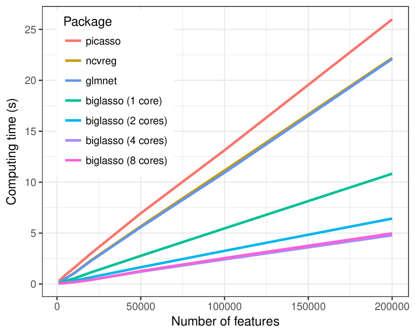
(a) Varying $p$, $n=1,000$.

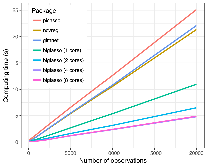
(b) Varying $n$, $p=10,000$.

Figure 2: Mean computing time (in seconds) of solving the lasso over a sequence 100 $\lambda$ values as a function of $p$ (Left) and $n$ (Right).

4.2.2 Real data

In this section, we compare the performance of the packages using diverse real data sets: (1) Breast cancer gene expression data (GENE); (2) MNIST handwritten image data (MNIST); (3) Cardiac fibrosis genome-wide association study data (GWAS); and (4) Subset of New York Times bag-of-words data (NYT). Note that for data sets MNIST and NYT, a different response vector is randomly sampled from a test set at each replication.

The size of the feature matrices and the average computing times are summarized in Table 3. In all four settings, biglasso was fastest at obtaining solutions, providing 2x to 3.8x speedup compared to glmnet and ncvreg, and 2x to 4.6x speedup compared to picasso.

Package	GENE	MNIST	GWAS	NYT
	$n=536$	$n=784$	$n=313$	$n=5,000$
	$p=17,322$	$p=60,000$	$p=660,495$	$p=55,000$
picasso	1.50 (0.01)	6.86 (0.06)	34.00 (0.47)	44.24 (0.46)
ncvreg	1.14 (0.02)	5.60 (0.06)	31.55 (0.18)	32.78 (0.10)
glmnet	1.02 (0.01)	5.63 (0.05)	23.23 (0.19)	33.38 (0.08)
biglasso	0.54 (0.01)	1.48 (0.10)	17.17 (0.11)	14.35 (1.29)

Table 3: Mean (SE) computing time (seconds) for solving the lasso along a sequence of 100 $\lambda$ values.

4.3 Computational efficiency: Logistic regression

4.3.1 Simulated data

Similar to Section 4.2, here we first illustrate that biglasso is faster than other packages in fitting the logistic regression model with simulated data. The true data-generating model is: $y_{i}\sim Bin(1,prob);\textrm{logit}(prob)=\mathbf{x}_{i}\bm{\beta}$, where each entry of $\mathbf{x}_{i}$ is i.i.d. sampled from standard Gaussian distribution. Again, two cases – varying $p$ and varying $n$ – are considered. 20 true features are randomly chosen and their coefficients are sampled from Unif[-1, 1].

Figure 3 summarizes the mean computing times of solving the lasso-penalized logistic regression over a sequence of 100 values of $\lambda$ by the four packages. In all the settings, biglasso (1 core) is around 1.5x faster than glmnet and ncvreg, and more than 3x faster than picasso. Parallel computing with 4 cores using biglasso reduces the computing time by half.

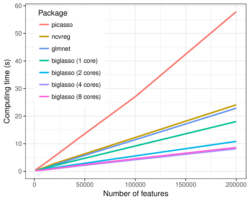
(a) Varying $p$, $n=1,000$.

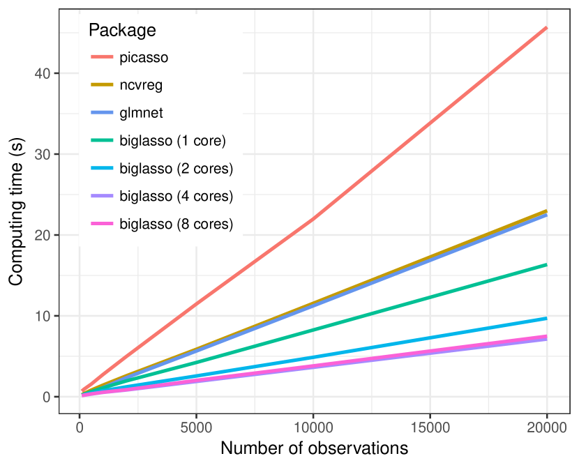
(b) Varying $n$, $p=10,000$.

Figure 3: Mean computing time (in seconds) of solving the lasso-penalized logistic regression over a sequence 100 $\lambda$ values as a function of $p$ (Left) and $n$ (Right).

4.3.2 Real data

We also compare the computing time of biglasso with other packages for fitting lasso-penalized logistic regression based on four real data sets: (1) Subset of Gisette data set; (2) P53 mutants data set; (3) Subset of NEWS20 data set; (4) Subset of RCV1 text categorization data set. The P53 data set can be found on the UCI Machine Learning Repository website (Lichman, 2013). The other three data sets are obtained from the LIBSVM data repository site.

Table 4 presents the dimensions of the data sets and the mean computing times. Again, biglasso outperforms all other packages in terms of computing time in all the real data cases. In particular, It’s significantly faster than picasso with the speedup ranging from 2 to 5.5 times (for P53 data and RCV1 data, respectively). On the other hand, compared to glmnet or ncvreg, biglasso doesn’t provide as much improvement in speed as in the linear regression case. The main reason is that safe rules for logistic regression do not work as well – they are more computationally expensive and less powerful in discarding inactive features – as safe rules for linear regression.

	Gisette	P53	NEWS20	RCV1
Package	$n=5,000$	$n=16,592$	$n=2,500$	$n=5,000$
	$p=5,000$	$p=5,408$	$p=96,202$	$p=47,236$
picasso	6.15 (0.03)	19.49 (0.06)	68.92 (8.17)	53.23 (0.13)
ncvreg	5.50 (0.03)	10.22 (0.02)	38.92 (0.56)	19.68 (0.07)
glmnet	3.10 (0.02)	10.39 (0.01)	25.00 (0.16)	14.51 (0.04)
biglasso	2.02 (0.01)	9.47 (0.02)	18.84 (0.22)	9.72 (0.04)

Table 4: Mean (SE) computing time (in seconds) for solving the lasso-penalized logistic regression along a sequence of 100 $\lambda$ values on real data sets.

4.4 Validation

To validate the numerical accuracy of our implementation, we contrast the model fitting results from biglasso to those from glmnet based on the following relative difference criterion:

$$RD(\lambda)=\frac{\hat{Q}(\hat{\bm{\beta}}^{B};\lambda)-\hat{Q}(\hat{\bm{\beta}}^{G};\lambda)}{\hat{Q}(\hat{\bm{\beta}}^{G};\lambda)},$$

where $\hat{\bm{\beta}}^{B}$ and $\hat{\bm{\beta}}^{G}$ denote the biglasso and glmnet solutions, respectively. Four real data sets are considered, including MNIST and GWAS for linear regression, and P53 and NEWS20 for logistic regression. For the GWAS and P53 data sets, we obtain 100 $RD$ values, one of each value of $\lambda$ along the regularization path. For the MNIST and NEWS20 data sets, we obtained solutions for 20 different response vectors, each with a path of 100 $\lambda$ values, resulting in 2,000 $RD$ values.

Table 5 presents the summary statistics of $RD(\lambda)$ for the 4 real data sets. For both linear and logistic regression cases, all values of $RD(\lambda)$ values are extremely close to zero, demonstrating that biglasso and glmnet converge to solutions with virtually identical values of the objective function.

Statistic	Linear regression		Logistic regression
	MNIST	GWAS	P53	NEWS20
Minimum	-7.7e-3	-3.9e-4	-6.4e-3	-1.6e-3
$1^{st}$ Quantile	-1.6e-3	-2.7e-5	1.7e-5	-2.2e-4
Median	-9.5e-4	1.6e-4	2.0e-4	-1.1e-4
Mean	-1.1e-3	8.3e-4	2.2e-4	-1.2e-4
$3^{rd}$ Quantile	-1.3e-4	1.3e-3	7.7e-4	1.0e-10
Maximum	4.2e-3	4.2e-3	2.0e-4	2.2e-3

Table 5: Summary statistics of $RD(\lambda)$ based on real data sets.

5 Data analysis example

In this section, we illustrate the usage of biglasso with a real data set colon included in biglasso. The colon data contains contains expression measurements of 2,000 genes for 62 samples from patients who underwent a biopsy for colon cancer. There are 40 samples from positive biopsies (tumor samples) and 22 from negative biopsies (normal samples). The goal is to identify genes that are predictive of colon cancer.

biglasso package has two main model-fitting R functions as below. Detailed syntax of the two functions can be found in the package reference manual.

• biglasso: used for a single model fitting.

• cv.biglasso: used for performing cross-validation and selecting parameter $\lambda$.

We first load the data: X is the 62-by-2000 raw data matrix, and y is the response vector with 1 indicating tumor sample and 0 indicating normal sample.

library(biglasso) data(colon) X <- colon$Xy<-colon$y dim(X) X[1:5, 1:5] y

The output of the R snippet above is as follows. > dim(X) [1] 62 2000 > X[1:5, 1:5] Hsa.3004 Hsa.13491 Hsa.13491.1 Hsa.37254 Hsa.541 t 8589.42 5468.24 4263.41 4064.94 1997.89 n 9164.25 6719.53 4883.45 3718.16 2015.22 t 3825.71 6970.36 5369.97 4705.65 1166.55 n 6246.45 7823.53 5955.84 3975.56 2002.61 t 3230.33 3694.45 3400.74 3463.59 2181.42 > y [1] 1 0 1 0 1 0 1 0 1 0 1 0 1 0 1 0 1 0 1 0 1 0 1 0 1 1 1 1 1 1 1 1 1 1 1 1 1 [38] 1 0 1 1 0 0 1 1 1 1 0 1 0 0 1 1 0 0 1 1 1 1 0 1 0

5.1 Set up the design matrix

It’s important to note that biglasso requires that the design matrix X must be a big.matrix object - an external pointer to the data. This can be done in two ways:

• If the size of X is small, as in this case, a big.matrix object can be created via: X.bm <- as.big.matrix(X) X.bm is a pointer to the data matrix, as shown in the following output. > str(X.bm) Formal class ’big.matrix’ [package "bigmemory"] with 1 slot ..@ address:<externalptr> > dim(X.bm) [1] 62 2000 > X.bm[1:5, 1:5] Hsa.3004 Hsa.13491 Hsa.13491.1 Hsa.37254 Hsa.541 t 8589.42 5468.24 4263.41 4064.94 1997.89 n 9164.25 6719.53 4883.45 3718.16 2015.22 t 3825.71 6970.36 5369.97 4705.65 1166.55 n 6246.45 7823.53 5955.84 3975.56 2002.61 t 3230.33 3694.45 3400.74 3463.59 2181.42

• If the size of the data is large, the user must create a file-backed big.matrix object via the utility function setupX in biglasso. Specifically, setupX reads the massive data stored on disk, and creates memory-mapped files for that data set. Section 6 demonstrates this case. A detailed example can also be found in the package vignettes.

5.2 Single fit and cross-validation

After the setup, we can now fit a lasso-penalized logistic regression model. fit <- biglasso(X.bm, y, family = "binomial") By default, our proposed screening rule “SSR-Slores” is used to accelerate the model fitting.

The output object fit is a list of model fitting results, including the sparse matrix beta. Each column of beta corresponds to the estimated coefficient vector at one of the 100 values of $\lambda$.

In practice, cross-validation is typically conducted to select $\lambda$ and hence the model with the best prediction accuracy. The following code snippet conducts a 10-fold (default) cross-validation using parallel computing with 4 cores. cvfit <- cv.biglasso(X.bm, y, family = "binomial", seed = 1234, ncores = 4) par(mfrow = c(2, 2), mar = c(3.5, 3.5, 3, 1), mgp = c(2.5, 0.5, 0)) plot(cvfit, type = "all")

Figure 4 displays the cross-validation curves with standard error bars. The vertical, dahsed, red line indicates the $\lambda$ value corresponding to the minimum cross-validation error.

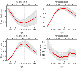
Figure 4: The cross-validation curves with standard error bars.

Similar to glmnet and other packages, biglasso provides coef, predict, and plot methods for both biglasso and cv.biglasso objects. Furthermore, cv.biglasso objects contain the biglasso fit to the full data set, so one can extract the fitted coefficients, make predictions using it, etc., without ever calling biglasso directly. For example, the following code displays the full lasso solution path, with a red dashed line indicating the selected $\lambda$ (Figure 5).

plot(cvfit$fit)abline(v=log(cvfit$lambda.min), col = 2, lty = 2)

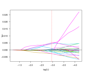
Figure 5: The solution path of lasso-penalized logistic regression model for the colon data.

The coefficient estimates at the selected $\lambda$ can be extracted via: coef: coefs <- as.matrix(coef(cvfit)) Here we output only nonzero coefficients: > coefs[coefs != 0, ] (Intercept) Hsa.8147 Hsa.36689 Hsa.42949 Hsa.22762 7.556421e-01 -6.722901e-05 -2.670110e-03 -3.722229e-04 1.698915e-05 Hsa.692.2 Hsa.31801 Hsa.3016 Hsa.5392 Hsa.1832 -1.142052e-03 4.491547e-04 2.265276e-04 4.518250e-03 -1.993107e-04 Hsa.12241 Hsa.44244 Hsa.2928 Hsa.41159 Hsa.33268 -8.824701e-04 -1.565108e-03 9.760147e-04 7.131923e-04 -2.622034e-03 Hsa.6814 Hsa.1660 4.426423e-03 5.156006e-03

The predict method, in addition to providing predictions for a feature matrix X, has several options to extract different quantities from the fitted model, such as the number and identity of the nonzero coefficients: > as.vector(predict(cvfit, X = X.bm, type = "class")) [1] 1 0 1 0 1 0 1 0 1 0 1 0 1 0 1 0 1 0 1 0 1 0 1 0 1 1 1 1 1 1 1 1 1 [34] 1 1 1 1 1 0 1 1 0 0 1 1 1 1 0 1 0 1 1 1 0 1 0 1 1 1 0 1 0 > predict(cvfit, type = "nvars") 0.0522 16 > predict(cvfit, type = "vars") Hsa.8147 Hsa.36689 Hsa.42949 Hsa.22762 Hsa.692.2 Hsa.31801 Hsa.3016 249 377 617 639 765 1024 1325 Hsa.5392 Hsa.1832 Hsa.12241 Hsa.44244 Hsa.2928 Hsa.41159 Hsa.33268 1346 1423 1482 1504 1582 1641 1644 Hsa.6814 Hsa.1660 1772 1870

In addition, the summary method can be applied to a cv.biglasso object to extract useful cross-validation results: > summary(cvfit) lasso-penalized logistic regression with n=62, p=2000 At minimum cross-validation error (lambda=0.0522): ————————————————- Nonzero coefficients: 16 Cross-validation error (deviance): 0.77 R-squared: 0.41 Signal-to-noise ratio: 0.70 Prediction error: 0.177

6 Application: Big Data case

Perhaps the most important feature of biglasso is its capability of out-of-core computing. To demonstrate this, we use it to analyze data from a genome-wide association study of 2898 infants (1911 controls and 987 premature cases). The goal is to identify genetic risk factors for premature birth. After preprocessing, 1,339,511 SNP (single-nucleotide polymorphism) measurements are used as features. The size of the resulting feature matrix is over 31 GB data, which is nearly 2x larger than the installed 16 GB RAM.

In this Big Data case, the data is stored in an external file on the disk. To use biglasso, memory-mapped files are first created via the following command.

X <- setupX(filename = "gwas_data.raw")

This command creates two files in the current working directory: (1) a memory-mapped file cache of the data, gwas_data.bin; and (2) a descriptor file, gwas_data.desc, that contains the backingfile description.

Note that this setup process takes a while if the data file is large (approximately 30 minutes in this case). However, this only needs to be done once, during data processing. Once the cache and descriptor files are generated, all future analyses using biglasso can use the X object. In particular, should one close R and open a new R session at a later date, X can be seamlessly retrieved by attaching its descriptor file as if it were already loaded into the main memory:

X <- attach.big.matrix("gwas_data.desc")

The object X returned from setupX or attach.big.matrix is a big.matrix object that is ready to be used for model fitting. Details about big.matrix and its related functions such as attach.big.matrix can be found in the reference manual of bigmemory package.

Note that the object X that we have created is a big.matrix object and is therefore stored on disk, not in RAM, but can be accessed as if it were a regular R object: > str(X) Formal class ’big.matrix’ [package "bigmemory"] with 1 slot ..@ address:<externalptr> > dim(X) [1] 2898 1339511 > X[1:10, 1:10] [,1] [,2] [,3] [,4] [,5] [,6] [,7] [,8] [,9] [,10] [1,] 1 1 0 0 1 1 1 0 1 1 [2,] 1 0 1 1 1 1 0 0 1 1 [3,] 1 0 1 1 1 1 0 0 1 1 [4,] 1 1 1 0 1 1 0 1 1 1 [5,] 1 1 0 1 1 1 0 1 1 1 [6,] 1 2 0 1 1 0 1 2 0 0 [7,] 1 2 0 0 1 0 1 2 1 0 [8,] 1 1 0 0 1 1 1 1 0 1 [9,] 1 0 1 1 1 1 0 0 0 1 [10,] 1 1 1 0 1 1 1 1 0 1 > table(y)

0 1 1911 987

Here we fit both sparse linear and logistic regression models with the lasso penalty over the entire path of 100 $\lambda$ values equally spaced on the scale of $\lambda/\lambda_{\max}$. The ratio of $\lambda_{\min}/\lambda_{\max}$ is set to be 0.1 for both models. Parallel computation with 4 cores is applied:

fit <- biglasso(X, y, ncores = 4) fit <- biglasso(X, y, family = "binomial", ncores = 4)

The above code, which solves the full lasso path for a 31 GB feature matrix, required 94 minutes for the linear regression fit and 146 minutes for the logistic regression fit on an ordinary laptop with 16 GB RAM installed. Figure 6 depicts the lasso solution path for the sparse linear regression model. The following code extracts the nonzero coefficient estimates and the number of selected variables of the lasso model when $\lambda=0.06$:

> coefs <- as.matrix(coef(fit, lambda = 0.06)) > coefs[coefs != 0, ] (Intercept) V78255 V289696 V602992 V602997 V602999 1.510095538 -0.004741494 -0.014724867 0.119765071 -0.093618971 0.020834021 V603003 V603034 V603042 V603065 V603067 V646528 -0.109134982 -0.046235902 -0.035036718 -0.042304267 -0.002034167 -0.019205575 V646544 V773260 V785150 V806320 V828475 V828488 -0.009025915 -0.012615210 -0.055444964 -0.011623245 0.075476347 0.021059097 V877563 V877564 V877624 V1000488 V1001897 V1136725 -0.044588035 -0.001164987 -0.020683459 -0.020375492 0.038315644 -0.021952476 > predict(fit, lambda = 0.06, type = "nvars") 0.06 23

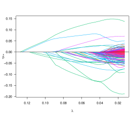
Figure 6: The solution path of the sparse linear regression model for the 31 GB GWAS data.

7 Conclusion

We developed a memory- and computation-efficient R package biglasso to extend lasso model fitting to Big Data. The package provides functions for fitting regularized linear and logistic regression models with both lasso and elastic net penalties. Equipped with the memory-mapping technique and more efficient screening rules, biglasso is not only is 1.5x to 4x times faster than existing packages, but consumes far less memory and, critically, enables users to fit lasso models involving data sets that are too large to be loaded into memory.

Appendix

Using the big data set in Section 6, we also conduct experiments to investigate the time savings by our newly proposed rule, SSR-BEDPP, compared to SSR.

Here we solve lasso-penalized linear regression over the entire path of 100 $\lambda$ values equally spaced on the scale of $\lambda/\lambda_{\max}$. We consider two cases in terms of $\lambda_{\min}$: (1) $\lambda_{\min}=0.1\lambda_{\max}$ as before; and (2) $\lambda_{\min}=0.5\lambda_{\max}$, as in practice there is typically less interest in lower values of $\lambda$ for very high-dimensional data such as this.

Since other packages cannot handle this data-larger-than-RAM case, we compare the performance of screening rules SSR and SSR-BEDPP based on biglasso. Table 6 summarizes the total computing time with the two rules under two cases with and without parallel computing. Clearly our proposed rule SSR-BEDPP is much more efficient in both cases. In particular, SSR-BEDPP is nearly 2.8x faster than SSR in Case 2.

Rule	$\lambda_{\min}/\lambda_{\max}=0.1$		$\lambda_{\min}/\lambda_{\max}=0.5$
	1 core	4 cores	1 core	4 cores
SSR	285	143	286	141
SSR-BEDPP	189	94	103	51

Table 6: The total computing time (in minutes) of solving the lasso-penalized linear regression along a sequence of 100 $\lambda$ values for 31 GB data on a laptop with 16 GB RAM.

References

- Angelosante and Giannakis (2009) Angelosante D, Giannakis GB (2009). “RLS-weighted Lasso for adaptive estimation of sparse signals.” In IEEE International Conference on Acoustics, Speech and Signal Processing, pp. 3245–3248.
- Bovet and Cesati (2005) Bovet DP, Cesati M (2005). Understanding the Linux kernel. O’Reilly.
- Breheny and Huang (2011) Breheny P, Huang J (2011). “Coordinate descent algorithms for nonconvex penalized regression, with applications to biological feature selection.” Annals of Applied Statistics, 5(1), 232–253.
- Fan et al. (2014) Fan J, Han F, Liu H (2014). “Challenges of big data analysis.” National Science Review, 1(2), 293–314.
- Friedman et al. (2010) Friedman J, Hastie T, Tibshirani R (2010). “Regularization paths for generalized linear models via coordinate descent.” Journal of Statistical Software, 33(1), 1.
- Ge et al. (2015) Ge J, Li X, Wang M, Zhang T, Liu H, Zhao T (2015). \pkgpicasso: Pathwise Calibrated Sparse Shooting Algorithm. \proglangR package version 0.5-4, URL https://CRAN.R-project.org/package=picasso.
- Huang and Pan (2003) Huang X, Pan W (2003). “Linear regression and two-class classification with gene expression data.” Bioinformatics, 19(16), 2072–2078.
- Kane et al. (2013) Kane MJ, Emerson J, Weston S (2013). “Scalable strategies for computing with massive data.” Journal of Statistical Software, 55(14), 1–19.
- Li et al. (2015) Li Y, Algarni A, Albathan M, Shen Y, Bijaksana MA (2015). “Relevance feature discovery for text mining.” IEEE Transactions on Knowledge and Data Engineering, 27(6), 1656–1669.
- Lichman (2013) Lichman M (2013). “UCI Machine Learning Repository.” URL http://archive.ics.uci.edu/ml.
- Lin et al. (2014) Lin Z, Kahng M, Sabrin KM, Chau DHP, Lee H, Kang U (2014). “Mmap: Fast billion-scale graph computation on a pc via memory mapping.” In IEEE International Conference on Big Data, pp. 159–164.
- Rao et al. (2010) Rao ST, Prasad E, Venkateswarlu N (2010). “A critical performance study of memory mapping on multi-core processors: An experiment with k-means algorithm with large data mining data sets.” International Journal of Computers and Applications, 1(9), 90–98.
- Tibshirani (1996) Tibshirani R (1996). “Regression Shrinkage and Selection via the Lasso.” Journal of the Royal Statistical Society Series B, 58(1), 267–288. ISSN 00359246.
- Tibshirani et al. (2012) Tibshirani R, Bien J, Friedman J, Hastie T, Simon N, Taylor J, Tibshirani RJ (2012). “Strong rules for discarding predictors in lasso-type problems.” Journal of the Royal Statistical Society Series B, 74(2), 245–266.
- Wang et al. (2015) Wang J, Wonka P, Ye J (2015). “Lasso Screening Rules via Dual Polytope Projection.” Journal of Machine Learning Research, 16, 1063–1101.
- Wang et al. (2014) Wang J, Zhou J, Liu J, Wonka P, Ye J (2014). “A safe screening rule for sparse logistic regression.” In Advances in Neural Information Processing Systems, pp. 1053–1061.
- Wright et al. (2009) Wright J, Yang AY, Ganesh A, Sastry SS, Ma Y (2009). “Robust face recognition via sparse representation.” IEEE Transactions on Pattern Analysis and Machine Intelligence, 31(2), 210–227.
- Zeng and Breheny (2016) Zeng Y, Breheny P (2016). \pkgbiglasso: Extending Lasso Model Fitting to Big Data. \proglangR package version 1.3-1, URL https://CRAN.R-project.org/package=biglasso.
- Zeng et al. (2017) Zeng Y, Yang T, Breheny P (2017). “Efficient Feature Screening for Lasso-Type Problems via Hybrid Safe-Strong Rules.” arXiv preprint arXiv:1704.08742.