Baryonic impact on the dark matter orbital properties of Milky Way-sized haloes

Abstract

We study the orbital properties of dark matter haloes by combining a spectral method and cosmological simulations of Milky Way-sized galaxies. We compare the dynamics and orbits of individual dark matter particles from both hydrodynamic and $N$-body simulations, and find that the fraction of box, tube and resonant orbits of the dark matter halo decreases significantly due to the effects of baryons. In particular, the central region of the dark matter halo in the hydrodynamic simulation is dominated by regular, short-axis tube orbits, in contrast to the chaotic, box and thin orbits dominant in the $N$-body run. This leads to a more spherical dark matter halo in the hydrodynamic run compared to a prolate one as commonly seen in the $N$-body simulations. Furthermore, by using a kernel based density estimator, we compare the coarse-grained phase-space densities of dark matter haloes in both simulations and find that it is lower by $\sim 0.5$ dex in the hydrodynamic run due to changes in the angular momentum distribution, which indicates that the baryonic process that affects the dark matter is irreversible. Our results imply that baryons play an important role in determining the shape, kinematics and phase-space density of dark matter haloes in galaxies.

1 Introduction

Within the cold dark matter (CDM) cosmology framework, it has been long known that collapsed haloes show a cuspy density distribution called Navarro-Frenk-White (NFW) profile (Navarro et al., 1997), as well as strongly triaxial shapes (Jing & Suto, 2002). For a self-gravitating system, there is no equilibrium in a thermodynamic sense (Lynden-Bell, 1967) that the system can rest on (Binney & Tremaine, 2008). The present-day properties of DM haloes depend on their evolutionary paths starting from cosmological initial conditions (see the example given by Arad & Lynden-Bell 2005). In the hierarchical growth picture, triaxial haloes naturally arise from halo mergers with the remnant shape closely connected to the orbits of the progenitors. Moore et al. (2004) found that mergers on radial orbits produce prolate systems while circular orbits result in oblate ones. However, the steep density slope in the centre as in the NFW profile (Navarro et al., 1997) does not necessarily originate from mergers. It was suggested from 1-D studies that a single mode gravitational collapse naturally produces a power-law density profile in the centre (e.g., Binney, 2004; Schulz et al., 2013; Colombi & Touma, 2014), although the central density slopes derived from these studies differ from each other. Steep cusps, on the other hand, are persistent during mergers (Dehnen, 2005) which possibly leads to an attractor (Syer & White, 1998; Loeb & Peebles, 2003), as suggested by numerical simulations (Angulo et al., 2016).

While recent works by Vogelsberger et al. (2008) and Abel et al. (2012) made progress in the study of DM using fine-grained phase-space density, our knowledge of the halo properties are mostly based upon collisionless $N-$body simulations. It has been suggested that baryons have a profound effect on the distribution of dark matter (Navarro et al., 1996; Lackner & Ostriker, 2010). The intrinsic shape of DM haloes is closely linked with the orbital properties of its constituents (e.g. Schwarzschild, 1979; Barnes & Hernquist, 1996; Holley-Bockelmann et al., 2001; Jesseit et al., 2005; Hoffman et al., 2010). In a 3-D non-spherical system such that the potential is not fully integrable, only energy is conserved. Orbits in such potentials are usually not closed and several major orbital families have been long recognized (e.g. Schwarzschild, 1979; Statler, 1987). Among these orbit families, box orbits, which are the backbone of triaxial systems, can pass quite close to the potential centre and be deflected by a supermassive black hole (Gerhard & Binney, 1985). From this effect, over time, an original triaxial system can be shaped into a more spherical one. In galaxy mergers with gas cooling and star formation included, orbital families are also found to be sensitively dependent on the gas content (Barnes & Hernquist, 1996; Hoffman et al., 2010).

Recently, we studied the baryonic effects on DM properties by comparing a cosmological hydrodynamic simulation (C-4) of a Milky Way-sized galaxy with its dark matter only (DMO) counterpart (Zhu et al., 2016). We found the shape of the DM halo in the hydrodynamic simulation appears to be nearly spherical, in contrast to the oblate shape in the DMO run. The more spherical DM halo in the hydrodynamic simulation agrees with other studies using different numerical techniques and models. Some of the previous studies (e.g. Maccio’ et al., 2007; Debattista et al., 2008; Valluri et al., 2010; Bryan et al., 2012) have focused on the orbital properties of the halo using spectral techniques (Binney & Spergel, 1982; Laskar, 1993). While these studies agreed that a significant fraction of box orbits are replaced by short axis tube orbits when a baryonic disk is present, whether or not such a process is reversible remains under debate.

Using a controlled experiment including a growing and evaporating disk potential, Valluri et al. (2010) concluded that the change induced by baryons on the DM particle orbits critically depends on the radial distribution of baryons. More centrally concentrated baryons introduce changes in a more irreversible fashion. Thanks to the rapid developments within the past few years (e.g. Guedes et al., 2011; Agertz et al., 2011; Aumer et al., 2013; Marinacci et al., 2014), we can now study DM haloes from cosmological hydrodynamic simulations to better understand the impact of baryons on the DM distribution.

In this study, we apply an automatic orbit classification code called smile (Vasiliev, 2013), which uses a spectral method, to analyze the DM particle orbits of the Milky Way-sized halo studied in Zhu et al. (2016). Compared with previous studies, we use a more accurate representation of the potential field based on our cosmological simulations and a high order integration scheme which greatly improves the accuracy of indications of chaos. Moreover, the classification of orbits in our study further distinguishes resonant and thin orbits (Merritt & Valluri, 1999) from a broad box orbit family. Furthermore, the cosmological hydrodynamic simulation makes it possible to follow the build-up of the baryonic disk in detail, which itself has a manifestly complex angular momentum evolution (e.g. Grand et al., 2016). Possible coupling between the angular momentum of the baryonic disk and the DM halo is a critical process that determines whether or not the impact induced by baryons on the DM is reversible. Such a process, however, was not properly modeled in previous studies using a rigid body potential (Debattista et al., 2008; Valluri et al., 2010).

This paper is organized as follows. We describe our methods in Section 2 and present the main results in Section 3. We discuss resolution effects and the triaxial symmetry assumption on the orbital properties in Section 4, and summarize our findings in Section 5.

Figure 1: Orbital families considered in this study. From top left to bottom right: a SAT, an inner LAT, an outer LAT, a (2:$*$:3)-resonant orbit, a thin orbit and a regular box orbit.

Figure 2: A comparison of dark matter halo shape between the hydrodynamic and DMO simulations of the Aq-C halo. Top panel: the projected DM density maps of Aq-C haloes in the $x-z$ plane. Bottom panel: the corresponding halo shape parameters in terms of axial ratios ($b/a$ and $c/a$), and triaxiality parameter ($T\equiv(a^{2}-b^{2})/(a^{2}-c^{2})$) as a function of galactocentric distance $r$.

Figure 3: Frequency maps in the plane of $\Omega_{x}/\Omega_{z}$ and $\Omega_{x}/\Omega_{z}$ for the Aq-C-4 halo from both hydrodynamic (left column) and DMO (right column) simulations, respectively. The top panels show a larger range than the bottom ones. The dots indicate individual orbits color-coded by their binding energy $E_{\rm binding}=\Phi(r)+\mathbf{v}^{2}/2$. The three gray solid lines denote the locations for SAT, IAT and LAT orbits, which satisfy $\Omega_{x}\approx\Omega_{y}$, $\Omega_{x}\approx\Omega_{z}$ and $\Omega_{y}\approx\Omega_{z}$, respectively. The lower panels show zoom-in regions of the frequency maps shown in the top panel. For the DMO simulation, numerous thin and resonant orbits are visible in this region. For comparison, the orbits in the hydrodynamic simulation are sparsely populated in the same region.

2 Methods

2.1 Cosmological simulations

In this study, we use both hydrodynamical and dark matter only (DMO) cosmological simulations of the Milky Way-sized halo Aq-C-4 from Zhu et al. (2016) (referred to as the C-4 simulation hereafter). Both simulations have a mass resolution of $3.0\times 10^{5}\,\rm M_{\odot}$ for the DM component, while the hydrodynamic one has a mass resolution of $5.0\times 10^{4}\,\rm M_{\odot}$ for gas and stars, and it includes a comprehensive list of baryonic processes, such as metal cooling, star formation, feedback from both supernovae and active galactic nuclei, and stellar evolution. We have also included a set of simulations with a mass resolution 8 times lower than that of the C-4 runs (referred to as C-5 hereafter) to study the effects of resolution on the DM properties.

2.2 Orbit classification

We start from the snapshots at $z=0$ from the cosmological simulations to build a smooth potential model that we then use to follow the orbits of individual DM particles. We first locate the potential minimum and reorient the entire system to the principle axes determined by the mass distribution within 20 kpc of the potential minimum. For the hydrodynamic simulation, the stellar and gaseous components are included. The new $z$-direction in the C-4 simulation aligns almost perfectly with the orientation of its stellar disc.

We use the spherical-harmonic expansion method in smile using terms up to $n_{\rm rad}=12$ in the radial direction and $l_{\rm max}=6$, which are suitable for the total particle numbers in the halo. We further assume triaxial symmetry which leaves the coefficient of $Y^{m}_{l}(\theta,\phi)$ nonzero for even $l$ and $m$ terms. The above procedure closely follows the self-consistent field (SCF) method of Hernquist & Ostriker (1992) with the radial functional form replaced by a non-parametric density estimator using splines, which increases the accuracy of the approximations to the underlying potential/force field. In total, $\sim 8,700,000$ DM particles together with $\sim 3,800,000$ gas particles and $\sim 2,300,000$ star particles are evolved for C-4 simulation. We then use the position and velocity information of the DM particles selected from the snapshots as “tracers". In total, we select all the $\sim 300,000$ DM particles within $500$ kpc from the galaxy center for C-4 simulation (both hydrodynamic and DMO) and $\sim 35,000$ particles for C-5 simulation (which is about one eighth of the number in C-4 simulation). With the default eighth order Runga-Kutta algorithm and adaptive step sizes, we integrate each particle with 150 full orbits and the fractional error in energy conservation for the entire duration is below $10^{-5}$. The conservation of energy is a crucial step for the classification of different orbit families.

Following Binney & Spergel (1982), the coordinates of each orbit are analyzed as a function of time using Fourier spectra,

$$\\ x(t)=\sum_{k}A_{k}\exp(i\omega_{k}t).$$ (1)

The smile code employs the automatic method proposed by Carpintero & Aguilar (1998) to identify the location of peaks and extracts their amplitude in the discrete Fourier transform of the coordinates . For regular orbits, at most three frequencies are linearly independent while the frequency of all the other spectral lines can be expressed as the combination of the three fundamental frequencies $\Omega_{x}$, $\Omega_{y}$ and $\Omega_{z}$ as $\omega_{k}=l\Omega_{x}+m\Omega_{y}+n\Omega_{z}$, where $(l,m,n)$ are integer triplets.

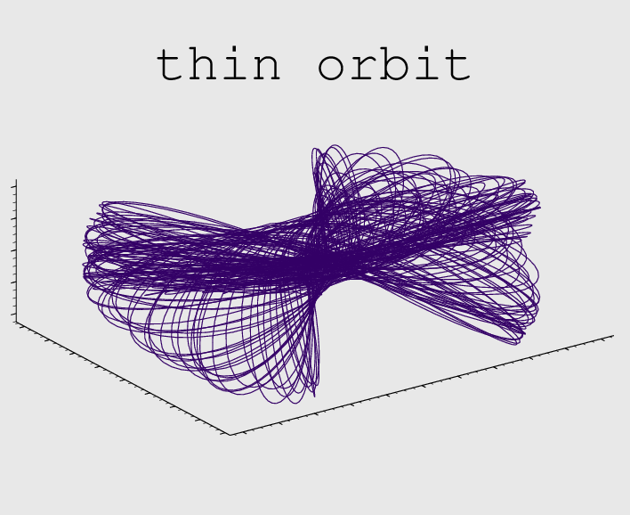
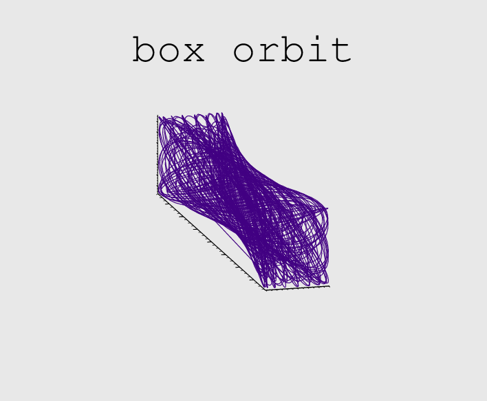
Subsequently, the classification of orbits is based on whether or not $\Omega_{x}$, $\Omega_{y}$ and $\Omega_{z}$ are commensurable. If the frequencies are not related through integer triplets, we have box orbits. On the other hand, they are called ($l,m,n$) thin orbits if the three fundamental frequencies satisfy the following resonant condition:

$$\\ l\Omega_{x}+m\Omega_{y}+n\Omega_{z}=0,$$ (2)

as they are confined on a membrane in configuration space (Merritt & Valluri, 1999).

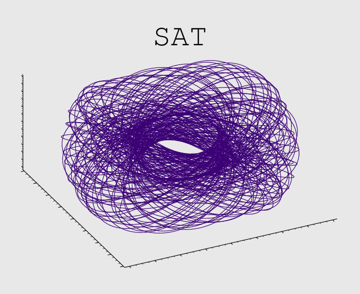
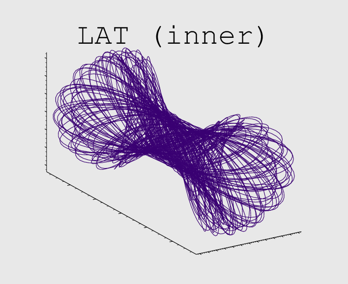
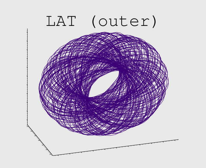
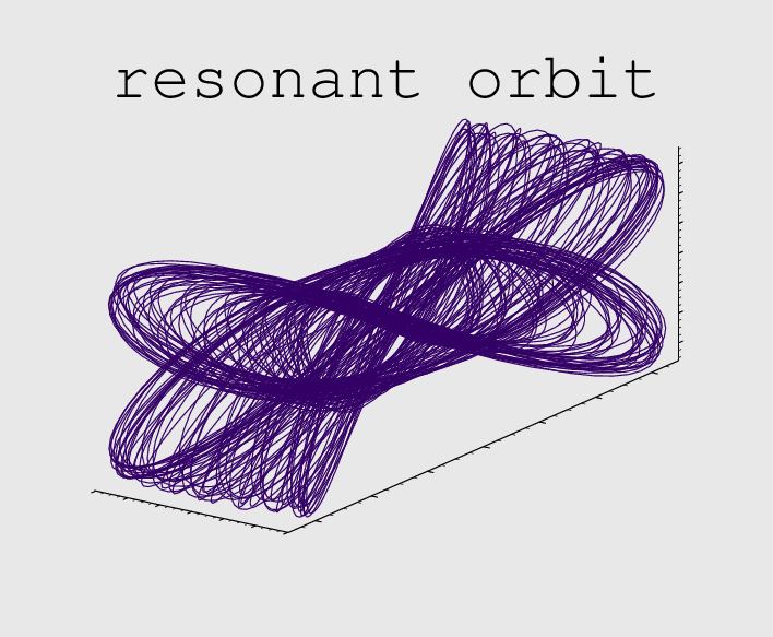
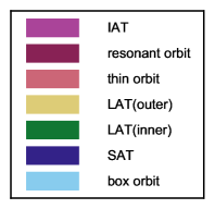
Among thin orbits we have “resonant orbits" where either $l$, $m$ or $n$ is 0. The most common subclass of resonant orbits is known as ‘tube orbits’ which correspond to a 1:1 resonance. We refer to the orbits with $\Omega_{x}\approx\Omega_{y}$ as short axis tubes (SAT, or Z-tubes) and those with $\Omega_{y}\approx\Omega_{z}$ as long axis tubes (LAT, or X-tubes). SAT and LAT orbits conserve the sign of the $z$ and $x$ components of angular momentum and hence they contribute net rotation around the $z$ and $x$ axes. Loop orbits around the intermediate axis (IAT) in perfect ellipsoidal potentials are unstable. Long axis tubes are further classified as inner and outer long-axis tubes (Statler, 1987; Binney & Tremaine, 2008). In this study, we consider the following most common orbital families: (1) SAT, (2) inner LAT, (3) outer LAT, (4) resonant orbits, (5) thin orbits, and (6) boxes, as illustrated in Figure 1.

If the spectral lines cannot be expressed as the linear combination of at most three fundamental frequencies, they should be labelled as chaotic according to Carpintero & Aguilar (1998). Since smile doest not have a separate ‘chaotic’ orbital family, these orbits are often classified under the ‘box’ category and sometimes can be under ‘resonant’ or ‘thin’ with additional ‘chaotic’ attribute. The latter happens if the spectra lines are under the tolerance parameter $\epsilon$ for detecting the resonant condition:

$$\\ |n_{b}*\Omega_{a}-n_{a}*\Omega_{b}|\leq\epsilon,$$ (3)

where $\max{(n_{a},n_{b})}\leq 10$. To further study the chaotic properties of the orbits, smile computes the frequency diffusion rate $\Delta\Omega$ as the change of frequencies between the first and second halves of the interval ($\Omega_{k,1},\Omega_{k,2}$):

$$\\ \Delta\Omega=\frac{1}{3}\sum_{k}\frac{|\Omega_{k,1}-\Omega_{k,2}|}{(\Omega_{k,1}+\Omega_{k,2})/2}.$$ (4)

In addition, the Lyapunov exponent $\Lambda$ using a nearby orbit is employed to provide a more secure measurement of chaos. All of the above procedures, potential reconstruction, orbital integration and classification, are included in the smile code where the classification is automatic.

The following pseudocode describes the overall procedure of orbit classification:

1. Perform FFT of the spatial coordinates and identify spectral lines;

2. Find the leading frequencies: $\Omega_{x}$, $\Omega_{y}$ and $\Omega_{z}$ in each coordiantes;

3. Test the binary commensurable relation in Equation (3) between each pair of the leading frequencies;

   1. If no resonant relation in any pairs of the leading frequencies is detected, smile tests Equation (2) to determine whether or not the orbit is a ‘box’ or a ‘thin’ orbit;

   2. If there are resonant relations detected in the pairs of the leading frequencies, the orbit is labeled as ‘resonant’.

4. Test whether $L_{x}$, $L_{y}$, and $L_{z}$ switch from positive(negative) values to opposite sign during the course of the integration to determine the orbit is a ‘tube’ orbit or not.

5. Finally, smile tests the relations between the leading frequencies and the rest of the spectral lines in each coordinates to determine whether or not the additional ‘chaotic’ attribute should be added to the orbit classification.

For a thorough description of orbit analysis, we refer the reader to Vasiliev (2013).

2.3 Phase-space density estimation

Several assumptions are made in the above approach with the most important one being that the potential is frozen. It has been suggested that gas cooling and star formation can change box orbits into SAT (Barnes & Hernquist, 1996; Hoffman et al., 2010). It is not clear whether such changes can be reversed. With a complementary approach, we compute a numerical estimate of phase-space density $f(\mathbf{x},\mathbf{v})$ using the EnBiD code (Sharma & Steinmetz, 2006) for DM particles. An SPH-like kernel smoothing is applied to compute the phase-space density along an adaptive metric with an anisotropic kernel. Vass et al. (2009) have shown that this approach is able to reveal more detailed structures in DM halos in phase-space, which are related to the subhaloes and newly formed tidal streams from disrupted subhaloes, rather than using the spherically averaged quantity $Q$($\equiv\rho/\sigma^{3})$. As mixing (from phase mixing, chaotic mixing, as well as violent relaxation) occurs, the coarse-grained phase density $f$ decreases with time (Dehnen, 2005; Vass et al., 2009).

Figure 4: The orbital families and their radial distributions for the Aq-C-4 halo from both hydrodynamic (middle panel) and DMO (bottom panel) simulations, respectively. The color pie in the (top panel) represents the color scheme used to illustrate different orbital family.

Figure 5: Histograms of frequency diffusion rates for tube-like orbits (SAT, LAT and resonant orbits, top panel), box-like orbits (thin and box orbits, middle panel) and the entire orbit family (bottom panel) of the Aq-C-4 halo from both hydrodynamic (in blue color) and DMO (in red color) simulations, respectively. There is a one percent relative change between two halves of the interval for $\Delta\Omega\sim 0.01$.

Higher values of frequency diffusion rates correspond to more strongly chaotic orbits.

3 Results

3.1 Dark matter halo shape

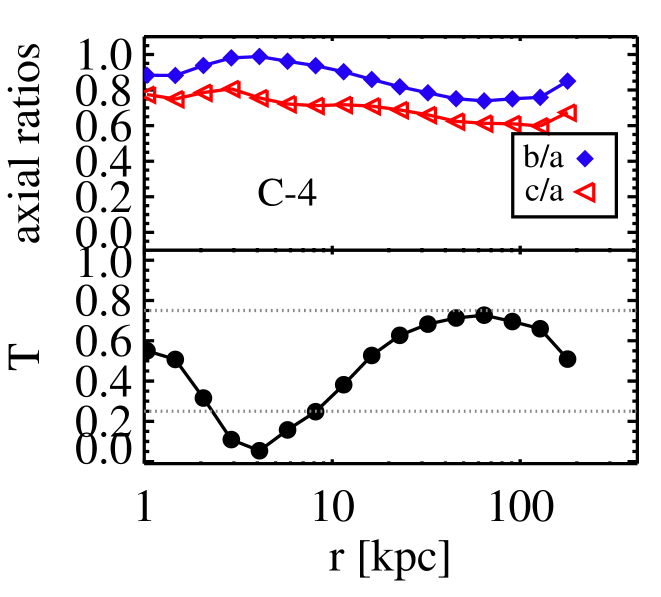
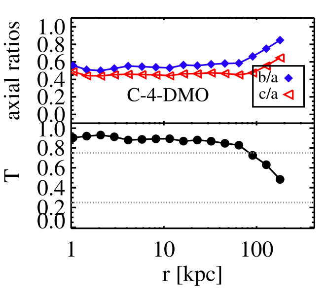
In order to study the distribution of DM particles, we apply a principal component analysis to compute the three axis parameters ${a}$, ${b}$ and ${c}$ based on the eigenvalues of the moment of inertia tensor for all the DM particles within a given shell (Zemp et al., 2011). The halo shape is quantified by the intermediate to major axis ratio, ${b/a}$, and the minor to major axis ratio, ${c/a}$, as well as a triaxiality parameter $T\equiv(a^{2}-b^{2})/(a^{2}-c^{2})$.

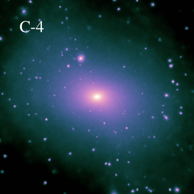
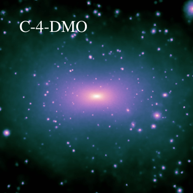
A comparison of the DM halo shape of Aq-C between the hydrodynamic and DMO simulations is shown in Figure 2. The impact of hydrodynamics on the distribution of DM is clearly visible in the images of the projected density maps in the top panels. For hydrodynamic simulations, haloes are more spherical while the DMO counterparts show a clear boxy shape. This is confirmed by the quantities ${b/a}$ and ${c/a}$ as a function of galactocentric distance $r$. Within 100 kpc, ${b/a}$ remains above 0.8 for the hydrodynamic simulation but around 0.6 for DMO simulations. The triaxiality parameter $T$ clearly indicates that the inner regions of the DM haloes in the hydrodynamic simulation are nearly spherical but those of the DMO simulation comprise a prolate ellipsoid. It is also evident that halo shape varies substantially as a function of $r$, which indicates that the global shapes of DM haloes are not perfect ellipsoids.

3.2 Orbital properties: frequency map and orbital family

As introduced in Section 2.2, frequency maps can be used to analyse the structure of the orbits based on the most prominent spectral lines in the frequencies of $\Omega_{x}$, $\Omega_{y}$ and $\Omega_{z}$ (Papaphilippou & Laskar, 1998; Valluri & Merritt, 1998; Valluri et al., 2012). We integrate individual orbits of DM particles using the mass distribution from the simulation snapshots as in Figure 2, then apply Fourier transforms to the orbit coordinates in each dimension.

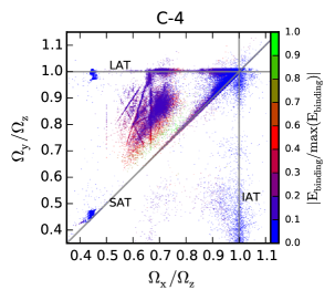
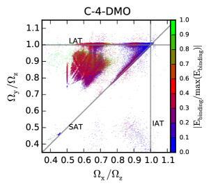
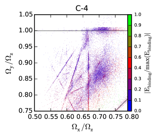
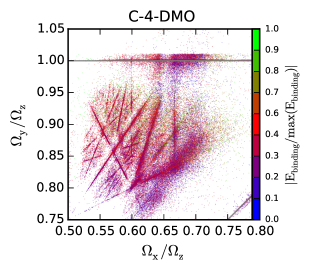
The resulting frequency maps from our simulations are shown in Figure 3. Both SAT and LAT are densely populated in the hydrodynamic and DMO simulations. A large fraction of orbits in C-4-DMO are clustered around $\Omega_{x}/\Omega_{y}\sim 0.6$ and $\Omega_{x}/\Omega_{z}\sim 0.8$, while the binding energy of each orbit is around half of the maximum binding energy $\frac{1}{2}\max(E_{\rm binding})$. Previous orbital classification has identified these orbits as box orbits while our classification will further separate thin orbits and resonant orbits from box orbits. For comparison, the frequency map of the Aq-C-4 halo shows that this region is not densely populated.

The bottom panels of Figure 3 highlight zoomed-in regions of the frequency space for the Aq-C-4 haloes. Many orbits are thin orbits in the DMO simulation, as in the bottom right panel, where many lines are heavily populated. In contrast, we find far fewer orbits distributed along the same lines in the hydrodynamic simulation. Moreover, we can also see that there are “gaps” along the various resonant relations such that only segments of the lines are populated in the DMO case. Physically, the “gaps" correspond to chaotic orbits where resonant relations overlap (Binney & Tremaine, 2008; Price-Whelan et al., 2016). While the orbits on the resonant lines are stable, the other orbits are irregular orbits for which the spectral method does not find well-defined frequencies.

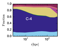
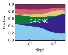
With the frequencies computed as in Figure 3, we can then assign orbital families to each individual orbit according to the method described in Section 2.2. Figure 4 summarises the fraction of orbital families as a function of $r$ for the DM haloes from both hydrodynamic and DMO runs.

Figure 4 shows the overall differences in the final DM haloes in the orbits of DM particles. Most important, the fraction of SAT orbits in the hydrodynamic simulation dominates the other orbital families. Within the central 10 kpc, more than 50 percent of orbits are classified as SAT. The fraction of SAT orbits in the C-4 simulation slowly decreases to 40 percent towards the outer regions of the halo. The fraction of box orbits in the hydrodynamic runs is subdominant, being slightly below 20 percent. For the DMO simulation, the central regions are occupied by other orbital families rather than SAT orbits. The relative weight of box orbits reaches up to 40 percent within the central 10 kpc while the contribution from inner LAT (which is almost absent in the hydrodynamic simulation), thin and resonant orbits also increases substantially. For the latter two orbital families, the combined contribution is around 20 percent in the DMO simulation, which is in contrast to their relative light weight in the hydrodynamic simulation. SAT orbits in the DMO simulation start to appear only at galactocentric distances beyond tens of kpc.

In the C-4 simulation, there is a very small fraction of orbits at $\sim 200$ kpc identified as IAT where $\Omega_{x}/\Omega_{z}\approx 1$. Such orbits are not stable in systems with perfect ellipsoidal potentials. However in more realistic situations where the orientations of the ellipsoidal shells are not well-aligned, such orbits can be present.

Box orbits (and thin orbits) are the most important constituents of triaxial systems (Merritt & Valluri, 1999). The radial distributions of orbital families in the two simulations are consistent with the halo shapes shown in Figure 2 as the triaxial halo in the C-4-DMO simulation is dominated by box, resonant and thin orbits.

3.3 Regular vs. chaotic orbits

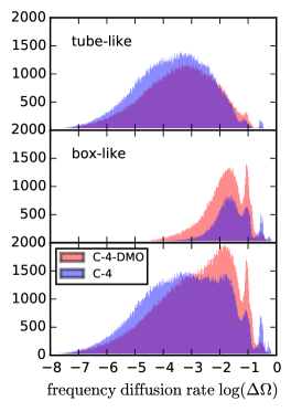
Regular orbits have definite frequencies in Fourier space. For chaotic orbits, their frequencies are broader than distinct lines. The frequency diffusion rate (Laskar, 1993) is a very useful tool for studying the chaotic properties of each orbit. The definition of the frequency diffusion rate in Equation (4) quantifies the relative change of frequencies within the time interval of hundreds of orbits. According to the analysis of Vasiliev (2013), the frequency diffusion rate is only an approximate indication of chaos as there is an intrinsic scatter of $\sim 0.5$ dex for $\Delta\Omega$. Nevertheless, the frequency diffusion rate correlates strongly with other chaos indicators such as the Lyapunov exponent $\Lambda$. For $\Delta\Omega\sim 0.01$, there is a one percent relative change in the orbital frequencies between the two halves of the interval.

Figure 5 shows the distribution of $\log(\Delta\Omega)$ for tube-like orbits such as SAT, LAT and resonant orbits, box-like orbits (thin and box orbits), and all the orbits we integrated for the Aq-C-4 halo from both hydrodynamic and DMO simulations. Not surprisingly, most of the tube-like orbits are regular ones with $\Delta\Omega$ well below 0.01. Chaotic orbits, those with $\Delta\Omega$ above 0.01, are mostly associated with thin and box orbits. Interestingly, the fraction of chaotic orbits in the hydrodynamic simulation is actually reduced rather than increased when compared to the DMO simulation as shown in the lower panel for the entire ensemble of orbits. We note there is a distinct peak of strong chaotic orbits in the hydrodynamic simulation with $\log(\Delta\Omega)\sim 0.5$. We have verified that these orbits are associated with DM particles at large galactocentric distances between 50 kpc and 250 kpc. Orbits in the central region of the DM halo in the hydrodynamic run are mostly regular ones, which are SAT orbits characterised with low-frequency diffusion rates.

3.4 Angular momentum

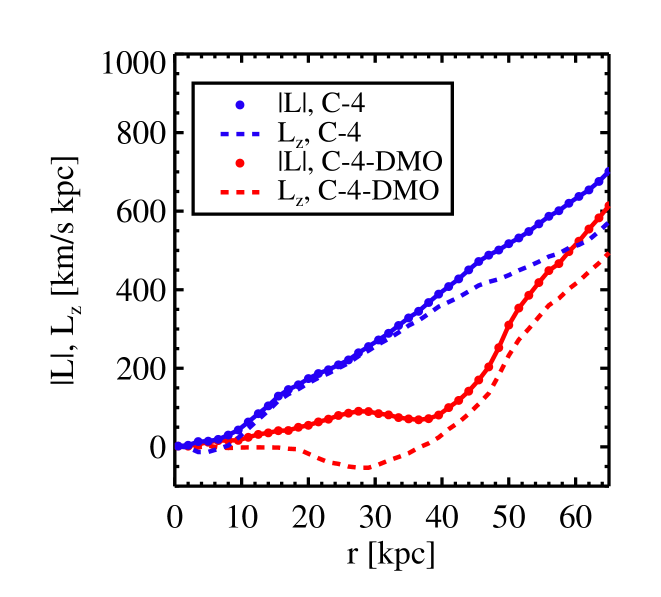
In addition to halo shapes and orbital families, as we discussed in the previous sections, hydrodynamic physics has a global impact on the angular momentum distribution in DM haloes. In Figure 6, we compare the mean angular momentum within concentric spherical shells of the Aq-C-4 halo from both hydrodynamic and DMO simulations. The angular momentum is calculated using the instantaneous position and velocity of each DM particle in the snapshot at $z=0$.

This plot shows a clear difference in both mean total angular momentum, $|\mathbf{L}|$, and the mean values of angular momentum in the $z$ direction, $L_{z}$ at all galactocentric distances between the hydrodynamic and DMO simulations. The central region of the DM halo in the hydrodynamic simulation shows clear net rotation as the mean values of $L_{z}$ are non-zero between $10$ and $30$ kpc, and it rises linearly up to $50$ kpc. This is also consistent with a large fraction of SAT orbits in the hydrodynamic run. For the DMO simulation, there is no coherent rotation along the $z$-axis within $20$ kpc as the $L_{z}$ curve lies close to zero. Beyond $20$ kpc, $L_{z}$ in DMO simulation switches from negative to positive at $\sim 40$ kpc.

Since the $z$-direction for the DM halo in the C-4 simulation is aligned with its stellar disc orientation, SAT orbits in the hydrodynamic simulation are either co-rotating or counterrotating with respect to the stellar disc. The sign of $L_{z}$ is positive beyond $10$ kpc, which means that most of the SAT orbits are corotating with the stellar disc. However within $10$ kpc, the fraction of counterrotating SAT orbits dominates over co-rotating SAT orbits, as the sign of $L_{z}$ is negative.

Figure 6: A comparison of the mean angular momentum at different galactocentric distance $r$ of the Aq-C-4 halo from both hydrodynamic (in blue color) and DMO (in red color) simulations, respectively. The mean total angular momentum, $|\mathbf{L}|$, is represented by the filled circles, while the mean values of angular momentum in the $z$ direction, $L_{z}$, is represented by the dashed curves.

Figure 7: A comparison of the coarse-grained phase-space density of DM particles at different galactocentric radius $r$ of the Aq-C-4 halo from both hydrodynamic and DMO simulations. The phase-space density $f$ is given in code units [$10^{10}\rm{M_{\odot}}/h\ (Mpc/h)^{-3}\ (km/s)^{-3}$]. The solid colored lines in all panels represent the 10th, 50th and 90th percentiles.

Figure 8: The orbital families and their radial distributions for the Aq-C-5 halo from both hydrodynamic and DMO simulations, respectively. The top panels show the orbital families with assumption of triaxial symmetry similar to the Aq-C-4 haloes in Figure 4, while the bottom panels without the triaxial symmetry assumption.

3.5 Phase-space density and the irreversible impact on DM due to baryons

While orbital analysis provides a powerful diagnosis of the structure of DM haloes, it is limited however due to the assumption that the potential is “frozen”. In this section, we use a numerical estimate of phase-space density as a complementary approach to study the evolution of DM particles. The “volume" that each particle occupies in phase space contains important information about their state and subsequent evolution.

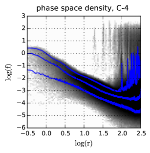
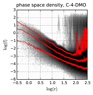
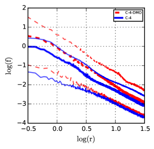
Figure 7 shows the numerical estimate of the coarse-grained phase-space density of DM particles as a function of galactocentric distance $r$ for both hydrodynamic and DMO simulations.

The overall radial distribution of the phase-space density of DM particles in our simulations is close to that obtained by Vass et al. (2009). High phase-space density regions correspond to subhaloes and newly formed “streams" from tidal disruption, which are preferentially located at large galactocentric distances. These are the “spikes” only found beyond 10 kpc. On the other hand, the central regions of DM haloes consist of a well-mixed smooth component (see also Diemand et al., 2008).

In Zhu et al. (2016), we compared the DM density profiles in the hydrodynamic and DMO simulations for the central haloes. We found that the difference between the two density profiles is fairly well captured by the adiabatic contraction model of Gnedin et al. (2004). The analysis of individual orbital properties in the present study indicates that the impact of dissipational processes (from gas cooling, star formation etc.) is more complicated. In particular, adiabatic changes of orbits are reversible.

The numerical value of $f$ can be viewed as a combination of mass density and local velocity dispersion. The right panel of Figure 7 illustrates significant differences between the hydrodynamic and DMO simulations. For DM particles in the central regions, their local velocity dispersion is greatly increased in the hydrodynamic simulation since the mass density in the hydrodynamic simulation is slightly higher than that in the DMO run (Zhu et al., 2016). The median values of $f$ in the hydrodynamic simulation are lowered by 0.5 dex compared to that in the DMO halo. In the very central regions, the 90th percentile $f$ of the hydrodynamic halo is close to the median values of $f$ in the DMO halo.

Such a difference in the phase-space density between the two simulations suggests an acceleration of mixing processes leading to a smooth component of DM haloes. Vass et al. (2009) have found that the phase density of the central regions of DM haloes gradually decreases from high redshift to low redshift. In addition, the difference in phase-space densities also suggests that the impact is not reversible. Debattista et al. (2008) and Valluri et al. (2010) show that if the central baryon mass concentration slowly evaporates, DM haloes can return to their original shape before the baryon mass is added. This reversal cannot be achieved in our fully cosmological hydrodynamics simulations if we slowly artificially remove the central mass distribution.

One important reason that the impact on the DM distribution due to baryons is irreversible owes to angular momentum exchange between the baryon and DM components. In Figure 6, the mean angular moment of each concentric DM shell in the hydrodynamic simulation is considerably larger than that of the DMO simulation. Moreover, within the central 30 kpc of the hydrodynamic DM halo, particles are circulating coherently along the $z-$axis, which is also the orientation of the stellar component. Such a coherent rotation of DM particles is not seen in the DMO simulation.

Another reason of the lower phase-space density $f$ in the hydrodynamic simulation lies in the combination of higher velocity dispersion and higher density of the DM particles compared with the DM run, and consequently the shorter dynamical time scale $t_{\rm dyn}\sim 1/\sqrt{G\rho}$. Unlike Debattista et al. (2008), the scattering of box orbits due to the baryonic disc is very likely to be the root cause here because the fraction of the box orbits in the DMO halo is greatly reduced in the hydrodynamic simulation.

Valluri & Merritt (1998) suggested that many of the stellar orbits can become chaotic in more axisymmetric systems when “dissipation" is added to triaxial potentials. This speculation is in the context of understanding the systematic differences in the light distributions between bright and faint elliptical galaxies. The same argument applies to the shapes of DM haloes. Interestingly, the fraction of chaotic orbits in the hydrodynamic simulation (shown in Figure 5) is actually lowered rather than increased relative to the dark matter only run. This is quite the opposite of what Valluri & Merritt (1998) suggest. We note that the low phase-space density in the C-4 simulation is consistent with an acceleration of orbital dynamics in the discussion of Valluri & Merritt (1998). Somehow, a new order is established in the hydrodynamic simulation.

4 Discussion

In Zhu et al. (2016), we emphasised the impact of baryonic processes on the DM distribution, focusing on the evolution of subhaloes using a high resolution cosmological hydrodynamic simulation of a Milky Way-sized galaxy by Marinacci et al. (2014). We showed that the combination of re-ionization and stronger tidal disruption in the hydrodynamic simulation leads to a different subhalo mass function and spatial distribution. The low mass end of the subhalo function is reduced by $\sim 50\%$ in the hydrodynamic simulation due to those two processes. The current study provides another rationale to use full hydrodynamic simulations, which are more expensive than $N$-body runs, to study the general properties of DM haloes.

4.1 Numerical resolution and the assumption of triaxial symmetry

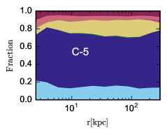
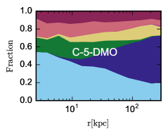
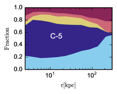
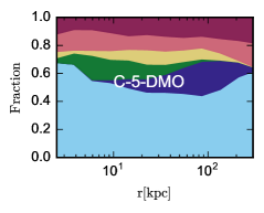
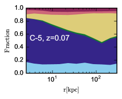
We have run the same spectral analysis on a lower resolution simulation in order to assess the impact of numerical resolution. Figure 8 shows the orbital classification of DM particles for C-5 haloes, with the left panel indicating the hydrodynamic halo and the right panel the DMO run. The fractions of different orbital families are quite consistent between the C-5 and C-4 simulations even though the mass resolution of the two suites differs by a factor of eight. This suggests that our results are numerically converged.

The mass distributions from the cosmological simulations are represented with analytical functions in our orbital analysis. In this study, we use spline functions in the radial direction and spherical harmonics as the angular basis. While our choice of the number of terms is able to match well the original potential which consists of point masses, the choice can lead to some quantitative differences nevertheless. The potential expansion we used also assumed triaxial symmetry with only odd $l$ and $m$ terms. To assess the impact of this assumption, we integrate the orbits in C-5 simulations without any constraint on odd or even $l,m$ terms. Similar to the middle panel of Figure 8, the lower panel shows the radial distribution of orbital families for the C-5 haloes but without the assumption of triaxial symmetry.

In fact, the radial distributions of the fractions of each orbital family are relatively insensitive to the assumption of triaxial symmetry. In particular, within the central 30 kpc the fraction number of SAT and box orbits in the hydrodynamic run is very close to that shown in the middle panel. Most of the differences are seen in the outer halo, where a significant of SAT orbits in the middle panel are replaced by various resonant, thin and box orbits. Similar changes can also be seen in the DMO halo where the SAT orbits in the triaxial symmetric potential are replaced by box orbits. In addition, the unstable IAT family (a negligible fraction for C-5 haloes in the middle panel of Figure 8) is absent when no triaxial symmetry is assumed.

We also have examined the impact of number of radial grids, using $n_{\rm rad}=20$ instead of our default value. The radial distribution of each orbital family in this test largely remains the same as the result obtained with $n_{\rm rad}=12$. This is consistent with Vasiliev (2013) who found that the density and force approximations using splines with a modest $n_{\rm rad}(\in[10,20])$ are sufficiently accurate.

4.2 The assumption of “frozen” potential

Figure 9: The radial distributions of the orbital families of the DM particles for the Aq-C-5 halo at redshifts $z=0.5$, $0.2$, and $0.07$. There are substantial changes in the orbital family distributions, and hence in the DM halo shape, from $z=0.5$ to $z=0.07$, and then to $z=0$ (upper left panel in Fig 8). In particular, a large fraction of IAT orbits at $z=0.5$ has disappeared, and the fraction of SAT orbits has increased significantly at $r\sim 100$ kpc. In contrast, the orbital family distribution in the inner halo shows much less evolution than that in the outer halo.

Another important assumption in our orbital classification is that the potential is frozen into a static one while in reality live DM halos are dynamically active because the mass assembly is ongoing process particularly in the outer halo (e.g., Wang et al., 2011; More et al., 2015).

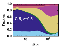
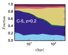
Figure 9 shows the orbital families and their radial distributions for the Aq-C-5 halo in the hydrodynamic simulation at three separate redshifts $z=0.5$, $0.2$, and $0.07$. For each snapshot, we repeat the same procedure of orbit integration and classification with smile. There are substantial changes in the orbital family distributions, and hence in the DM halo shape, from $z=0.5$ to $z=0.07$, and then to $z=0$. In particular, a large fraction of IAT orbits at $z=0.5$ has disappeared, and the fraction of SAT orbits has increased significantly in the outer halo since $z=0.5$.

Therefore, we conclude the assumption of a static potential is likely to have an impact on the orbital properties in the outer halo. One method to model of the evolution of the potential is to use some time-varying set of coefficients, as adopted by Lowing et al. (2011).

5 Conclusions

Current hydrodynamic simulations with comprehensive treatments of gas cooling and star formation have shown substantial modifications to the distribution of dark matter in galaxies. Following our study in Zhu et al. (2016), we have investigated the orbital properties of Milky Way-sized DM haloes by integrating the orbits of a large number of DM particles using spectral methods. Our key results are summarised as follows:

• DM haloes in hydrodynamic simulations appear more spherical than that of DMO simulations. The changes of halo shape in hydrodynamic simulations are reflected in the changes of orbital properties of individual particles. Box and thin orbits, which form the backbone of triaxiality in DM haloes, are replaced by SAT orbits in the hydrodynamic case.

• While we find a substantial fraction of inner LAT orbits in the inner part of the DMO halo, they are almost absent from the hydrodynamic halo.

• The fraction of chaotic orbits in the hydrodynamic halo is reduced compared to the DMO run. This is a result of a large number of box and thin orbits in the DMO halo being replaced by tube-like orbits, which are mostly regular.

• There is a net, coherent rotation of DM particles in the central regions in the hydrodynamic DM halo, which is absent in the DMO run. Within 10 kpc, the majority of DM particles on SAT obits are counter-rotating with respect to the stellar disc.

• In the central regions of the DM halo, the DM phase-space density is lowered by 0.5 dex when hydrodynamic processes are included. Considering the changes of angular momentum and the changes of the orbital families, this strongly suggests that the impact of baryons on the DM distribution is not reversible.

The spectral method and the classification of orbits using high resolution cosmological simulations as in this study can be easily extended to the core/cusp problem to offer additional insight into recent investigations (Madau et al., 2014; Oñorbe et al., 2015; Chan et al., 2015; Read et al., 2016). We plan to carry out such an analysis on high resolution cosmological simulations featuring bursty star formation using explicit stellar feedback models.

References

- Abel et al. (2012) Abel T., Hahn O., Kaehler R., 2012, MNRAS, 427, 61
- Agertz et al. (2011) Agertz O., Teyssier R., Moore B., 2011, MNRAS, 410, 1391
- Angulo et al. (2016) Angulo R. E., Hahn O., Ludlow A., Bonoli S., 2016, preprint, (arXiv:1604.03131)
- Arad & Lynden-Bell (2005) Arad I., Lynden-Bell D., 2005, MNRAS, 361, 385
- Aumer et al. (2013) Aumer M., White S. D. M., Naab T., Scannapieco C., 2013, MNRAS, 434, 3142
- Barnes & Hernquist (1996) Barnes J. E., Hernquist L., 1996, ApJ, 471, 115
- Binney (2004) Binney J., 2004, MNRAS, 350, 939
- Binney & Spergel (1982) Binney J., Spergel D., 1982, ApJ, 252, 308
- Binney & Tremaine (2008) Binney J., Tremaine S., 2008, Galactic Dynamics: Second Edition. Princeton University Press
- Bryan et al. (2012) Bryan S. E., Mao S., Kay S. T., Schaye J., Dalla Vecchia C., Booth C. M., 2012, MNRAS, 422, 1863
- Carpintero & Aguilar (1998) Carpintero D. D., Aguilar L. A., 1998, MNRAS, 298, 1
- Chan et al. (2015) Chan T. K., Kereš D., Oñorbe J., Hopkins P. F., Muratov A. L., Faucher-Giguère C.-A., Quataert E., 2015, MNRAS, 454, 2981
- Colombi & Touma (2014) Colombi S., Touma J., 2014, MNRAS, 441, 2414
- Debattista et al. (2008) Debattista V. P., Moore B., Quinn T., Kazantzidis S., Maas R., Mayer L., Read J., Stadel J., 2008, ApJ, 681, 1076
- Dehnen (2005) Dehnen W., 2005, MNRAS, 360, 892
- Diemand et al. (2008) Diemand J., Kuhlen M., Madau P., Zemp M., Moore B., Potter D., Stadel J., 2008, Nature, 454, 735
- Gerhard & Binney (1985) Gerhard O. E., Binney J., 1985, MNRAS, 216, 467
- Gnedin et al. (2004) Gnedin O. Y., Kravtsov A. V., Klypin A. A., Nagai D., 2004, ApJ, 616, 16
- Grand et al. (2016) Grand R. J. J., Springel V., Gómez F. A., Marinacci F., Pakmor R., Campbell D. J. R., Jenkins A., 2016, MNRAS, 459, 199
- Guedes et al. (2011) Guedes J., Callegari S., Madau P., Mayer L., 2011, ApJ, 742, 76
- Hernquist & Ostriker (1992) Hernquist L., Ostriker J. P., 1992, ApJ, 386, 375
- Hoffman et al. (2010) Hoffman L., Cox T. J., Dutta S., Hernquist L., 2010, ApJ, 723, 818
- Holley-Bockelmann et al. (2001) Holley-Bockelmann K., Mihos J. C., Sigurdsson S., Hernquist L., 2001, ApJ, 549, 862
- Jesseit et al. (2005) Jesseit R., Naab T., Burkert A., 2005, MNRAS, 360, 1185
- Jing & Suto (2002) Jing Y. P., Suto Y., 2002, ApJ, 574, 538
- Lackner & Ostriker (2010) Lackner C. N., Ostriker J. P., 2010, ApJ, 712, 88
- Laskar (1993) Laskar J., 1993, Physica D Nonlinear Phenomena, 67, 257
- Loeb & Peebles (2003) Loeb A., Peebles P. J. E., 2003, ApJ, 589, 29
- Lowing et al. (2011) Lowing B., Jenkins A., Eke V., Frenk C., 2011, MNRAS, 416, 2697
- Lynden-Bell (1967) Lynden-Bell D., 1967, MNRAS, 136, 101
- Maccio’ et al. (2007) Maccio’ A. V., Sideris I., Miranda M., Moore B., Jesseit R., 2007, preprint, (arXiv:0704.3078)
- Madau et al. (2014) Madau P., Shen S., Governato F., 2014, ApJ, 789, L17
- Marinacci et al. (2014) Marinacci F., Pakmor R., Springel V., 2014, MNRAS, 437, 1750
- Merritt & Valluri (1999) Merritt D., Valluri M., 1999, AJ, 118, 1177
- Moore et al. (2004) Moore B., Kazantzidis S., Diemand J., Stadel J., 2004, MNRAS, 354, 522
- More et al. (2015) More S., Diemer B., Kravtsov A. V., 2015, ApJ, 810, 36
- Navarro et al. (1996) Navarro J. F., Eke V. R., Frenk C. S., 1996, MNRAS, 283, L72
- Navarro et al. (1997) Navarro J. F., Frenk C. S., White S. D. M., 1997, ApJ, 490, 493
- Oñorbe et al. (2015) Oñorbe J., Boylan-Kolchin M., Bullock J. S., Hopkins P. F., Kereš D., Faucher-Giguère C.-A., Quataert E., Murray N., 2015, MNRAS, 454, 2092
- Papaphilippou & Laskar (1998) Papaphilippou Y., Laskar J., 1998, A&A, 329, 451
- Price-Whelan et al. (2016) Price-Whelan A. M., Johnston K. V., Valluri M., Pearson S., Küpper A. H. W., Hogg D. W., 2016, MNRAS, 455, 1079
- Read et al. (2016) Read J. I., Agertz O., Collins M. L. M., 2016, MNRAS, 459, 2573
- Schulz et al. (2013) Schulz A. E., Dehnen W., Jungman G., Tremaine S., 2013, MNRAS, 431, 49
- Schwarzschild (1979) Schwarzschild M., 1979, ApJ, 232, 236
- Sharma & Steinmetz (2006) Sharma S., Steinmetz M., 2006, MNRAS, 373, 1293
- Statler (1987) Statler T. S., 1987, ApJ, 321, 113
- Syer & White (1998) Syer D., White S. D. M., 1998, MNRAS, 293, 337
- Valluri & Merritt (1998) Valluri M., Merritt D., 1998, ApJ, 506, 686
- Valluri et al. (2010) Valluri M., Debattista V. P., Quinn T., Moore B., 2010, MNRAS, 403, 525
- Valluri et al. (2012) Valluri M., Debattista V. P., Quinn T. R., Roškar R., Wadsley J., 2012, MNRAS, 419, 1951
- Vasiliev (2013) Vasiliev E., 2013, MNRAS, 434, 3174
- Vass et al. (2009) Vass I. M., Valluri M., Kravtsov A. V., Kazantzidis S., 2009, MNRAS, 395, 1225
- Vogelsberger et al. (2008) Vogelsberger M., White S. D. M., Helmi A., Springel V., 2008, MNRAS, 385, 236
- Wang et al. (2011) Wang J., et al., 2011, MNRAS, 413, 1373
- Zemp et al. (2011) Zemp M., Gnedin O. Y., Gnedin N. Y., Kravtsov A. V., 2011, ApJS, 197, 30
- Zhu et al. (2016) Zhu Q., Marinacci F., Maji M., Li Y., Springel V., Hernquist L., 2016, MNRAS, 458, 1559