Black hole spectroscopy with coherent mode stacking

Abstract

The measurement of multiple ringdown modes in gravitational waves from binary black hole mergers will allow for testing fundamental properties of black holes in General Relativity, and to constrain modified theories of gravity. To enhance the ability of Advanced LIGO/Virgo to perform such tasks, we propose a coherent mode stacking method to search for a chosen target mode within a collection of multiple merger events. We first rescale each signal so that the target mode in each of them has the same frequency, and then sum the waveforms constructively. A crucial element to realize this coherent superposition is to make use of a priori information extracted from the inspiral-merger phase of each event. To illustrate the method, we perform a study with simulated events targeting the $\ell=m=3$ ringdown mode of the remnant black holes. We show that this method can significantly boost the signal-to-noise ratio of the collective target mode compared to that of the single loudest event. Using current estimates of merger rates we show that it is likely that advanced-era detectors can measure this collective ringdown mode with one year of coincident data gathered at design sensitivity.

Introduction. The recent detection of gravitational waves (GWs) emitted during the coalescence of binary black holes Abbott et al. (2016a, b) marked the beginning of the era of gravitational wave astronomy, a feat that heralds a boom of scientific discoveries to come. GWs not only provide a new window to our universe, they also offer a unique opportunity to test General Relativity (GR) in the dynamical and highly non-linear gravitational regime Yunes and Siemens (2013); Abbott et al. (2016c); Yunes et al. (2016); Abbott et al. (2016d); Lasky et al. (2016). One celebrated prediction of GR is the uniqueness, or “no-hair” property of vacuum black holes (BHs)  Israel (1967); Carter (1971); Hawking (1972); Robinson (1975); Cardoso and Gualtieri (2016): all isolated BHs are described by the Kerr family of solutions, each uniquely characterized by only its mass and spin . This property has many wide-ranging consequences, the two most relevant here being (a) that the spacetime of an isolated binary black hole (BBH) inspiral is uniquely characterized by a small, finite set of parameters identifying the two BHs in the binary and the properties of the orbit, and (b) that this same set of parameters uniquely determines the merger remnant and the full spectrum of its quasinormal mode (QNM) ringdown waveform.

This latter point forms the basis of black hole spectroscopy, where measurements of multiple ringdown modes are used to test this no-hair property. The idea is as follows. If the no-hair property holds, a measurement of the (complex) frequency of one QNM can be inverted to find a discrete set of possibilities for the spherical harmonic $(\ell,m)$ plus overtone number $n$ of the mode, and the BH mass $M$ and spin parameter $a=|\vec{S}|/M^{2}$, where $\vec{S}$ is the BH spin angular momentum. However, if we have a priori information about the objects that merged to form the perturbed BH, then we also have information about the dominant $(\ell,m,n)$ QNM, and the measurement of its complex frequency then provides information about the mass and spin of the perturbed object. The measurement of any additional QNM frequencies then overconstrains this mass and spin measurement, providing independent tests of the no-hair property. Naturally, the results of such tests can then be leveraged to place constraints on (or to detect) non-Kerr BHs in modified gravity theories, exotic compact objects, the presence of exotic/unexpected matter fields, etc. (e.g. Dreyer et al. (2004); Berti et al. (2006a); Kamaretsos et al. (2012); Gossan et al. (2012); Jackiw and Pi (2003); Alexander and Yunes (2009); Yunes and Pretorius (2009a); Yagi et al. (2012); Campbell et al. (1992); Kanti et al. (1996); Yunes and Stein (2011); Pani and Cardoso (2009); Yunes and Stein (2011); Pani et al. (2011); Ayzenberg and Yunes (2014); Brito et al. (2013)).

In fact, aLIGO has already given us a “zeroth-order” test of the no-hair property from event GW150914: the inspiral only portion of the signal was matched to a best-fit numerical relativity template, giving an estimate of the mass and spin of the remnant, and informing that the waveform shortly after peak amplitude should be dominated by the fundamental harmonic of the $(\ell,m)=(2,2)$ QNM (“22-mode” for short); this was consistent with the independently measured properties of the post-merger signal Abbott et al. (2016b). More stringent tests of the no-hair property of the final BH require observation of sub-leading QNMs . This is challenging using individual merger events given how weak these sub-leading modes are relative to the primary mode Berti et al. (2016); Bhagwat et al. (2016). For example, GW150914 has a ringdown signal-to-noise ratio (SNR) of $\approx 7$, but a ringdown SNR upwards of $45$ would have been needed to detect the first sub-leading QNM Gossan et al. (2012); Berti et al. (2007a). Thus detection of such modes in individual events will require third generation GW detectors, as even a loud GW150914-like event at aLIGO’s design sensitivity would have a ringdown SNR of $\approx 20$ Berti et al. (2016). On the other hand, many such events are expected after years of operation, leading us to consider how the information from multiple detections could be used to extract faint signals from a population of events.

Here then, we propose a way to coherently combine (or “stack”) multiple, high total SNR (low ringdown SNR) binary BH coalescence events, to boost the detectability of a chosen secondary QNM mode. An earlier study in Meidam et al. (2014) considered a similar problem, though their approach effectively amounted to an incoherent assembly of ringdown signals, where, all else being equal, one expects $N^{1/4}$ scaling of the SNR for $N$ events, compared to $N^{1/2}$ for a coherent method (see Supplemental Material for more details). Key to achieving coherent stacking is using information gleaned from the inspiral portion of each event to predict the relative phases and amplitudes of the ringdown modes excited in the remnant.

Signal stacking. Given a set of BBH coalescence observations, we first select the loudest subset, here taken to consist of the signals with ringdown SNR in the primary 22-mode alone of $\rho_{22}>8$. Based on the studies in Berti et al. (2006a, 2007a); London et al. (2014); Bhagwat et al. (2016); Buonanno et al. (2007); Berti et al. (2007b) the 33-mode is typically one of the next loudest ringdown modes. Therefore, we concentrate on the 33-mode as a target for our analysis, although the methodology presented here is generally applicable to other modes, as well as other features common to a population of GW events. Similar to the analysis in Berti et al. (2016); Bhagwat et al. (2016), we use the two-mode approximation to describe each detected ringdown signal $s_{j}(t)$ :

$$s_{j}=n_{j}+h_{22,j}+h_{33,j}\,,$$ (1)

where the subscript $j$ refers to the $j$th event, $n_{j}$ is the corresponding detector noise, and $h_{\ell m,j}$ is a ringdown mode of the form (for $t>0$)

$$h_{\ell m,j}(t)=A_{\ell m,j}e^{-\gamma_{\ell m,j}t}\sin(\omega_{\ell m,j}\,t-\phi_{\ell m,j})\,.$$ (2)

For each ringdown mode, $(\omega_{\ell m,j}+i\gamma_{\ell m,j})$ is its complex frequency, $A_{\ell m,j}$ its real amplitude, and $\phi_{\ell m,j}$ its constant phase offset.

Next, each entire $j$th signal is fitted to inspiral-merger-ringdown (IMR) waveform models in GR to accurately extract certain binary parameters that characterize the inspiral (e.g. the individual masses and spins). Using this, we can compute the QNM frequencies, phase offsets and amplitudes for all modes as expected in GR (the extrinsic parameters, such as the polarization and inclination angles do not affect the phase difference between the 22- and $\ell\ell$-modes ($\ell>2$) , as we discuss in the Supplemental Materials). This is a key ingredient of our coherent mode stacking, as we need to properly align the phase offsets $\phi_{33,j}$ and frequencies $\omega_{33,j}$ of the targeted modes to achieve optimal improvement in SNR relative to a single event analysis.

To perform the alignment, out of the set of $N$ events, we arbitrarily pick one (e.g. the $i$th one) as the base case, and shift/rescale all others to give the same expected secondary mode phase offset $\phi_{33,i}\equiv\phi_{33}$ and frequency $\omega_{33,i}\equiv\omega_{33}$. Specifically, we scale and shift each signal in time via ${\bf s}_{j}(t)\equiv s_{j}(t/\alpha_{j}+\Delta_{j})$, with $\alpha_{j}\equiv\omega_{33,j}/\omega_{33}$ and $\Delta_{j}\equiv(\phi_{33,j}-\phi_{33})/\omega_{33,j}$.

We are now ready to combine the individual signals. For convenience we work in the frequency domain, denoting the Fourier transform of a function $g(t)$ by $\tilde{g}(f)$. The Fourier transform of Eq. (2) is given by Berti et al. (2007a)

$$\tilde{h}_{\ell m,j}(f)=A_{\ell m,j}\frac{\omega_{\ell m,j}\cos\phi_{\ell m,j}-(\gamma_{\ell m,j}-i\,\omega)\sin\phi_{\ell m,j}}{\omega^{2}_{\ell m,j}-\omega^{2}+\gamma_{\ell m,j}^{2}-2i\,\omega\,\gamma_{\ell m,j}}$$ (3)

with $\omega=2\pi f$ the angular Fourier frequency. In the frequency domain, the secondary mode alignment of Eq. (1) is achieved via $\tilde{{\bf s}}_{j}(f)\equiv\alpha_{j}e^{i\omega\Delta_{j}\alpha_{j}}\tilde{s}_{j}(\alpha_{j}f)$. We then sum up these phase- and frequency-aligned signals to obtain our composite signal: $\tilde{{\bf s}}=\sum_{j}c_{j}\tilde{{\bf s}}_{j}\equiv\tilde{\bf n}+\tilde{\bf h}_{22}+\tilde{\bf h}_{33}$, where the identification of $\tilde{\bf n}$, $\tilde{\bf h}_{22}$ and $\tilde{\bf h}_{33}$ is obvious, and we describe later how to optimize the choice of weight constants $c_{j}$. If the frequencies and phase offsets are known exactly, $\tilde{\bf h}_{33}$ contains a single oscillation frequency $\omega_{33}$, and $\tilde{\bf h}_{22}$ contains a family of modes with (rescaled) frequencies $\in(0.623,2/3)\omega_{33}$ as the dimensionless BH spin $a$ ranges from $0-1$ Berti et al. (2006a); Yang et al. (2012).

Parameter uncertainty. Equation (1) decomposes a measured event into a true underlying signal and detector noise. The rescaling we have just described makes crucial use of parameters of the signal during the IMR phase, which can only be estimated to within some uncertainty, and this will introduce what we call “parameter estimation noise” $n_{h}$, that we will add to the composite signal $\tilde{\bf s}$. We investigate the role of this uncertainty here, leaving detailed derivations of some of the conclusions to the Supplemental Materials.

Parameter uncertainty produces two main sources of parameter estimation noise $n_{h}$. The first arises from subtracting an imperfectly-estimated ${\bf h}_{22}$ from the data. This noise source has frequency components quite close to the scaled frequencies $\omega_{22,j}$, which (in relative terms, when comparing to $\omega_{33,j}$) are far from $\omega_{33}$; the latter is the frequency at which $\tilde{\bf{h}}_{33}$ peaks, and thus, the impact of this noise source on $\rho_{33}$ is small. The second noise source is due to the imperfect scaling and alignment of the $33$ mode, which is resonant at frequency $\omega_{33}$.

Let us denote any variable with a prime as the maximum likelihood estimator, i.e. $Y^{\prime}=Y+\delta Y$, with $Y$ the true (scaled or not) value, and $\delta Y$ the corresponding uncertainty in its estimation. With this, the time domain, estimated composite GW signal is

$${\bf h}_{22}^{\prime}={\rm Im}\left\{\sum_{j}{\bf A}^{\prime}_{22,j}\,e^{i(\Lambda^{\prime}_{22,j}t-\Phi^{\prime}_{22,j})}\right\}\,,$$

$${\bf h}_{33}^{\prime}={\rm Im}\left\{e^{i(\omega_{33}t-\phi_{33})}\sum_{j}{\bf A}^{\prime}_{33,j}\,e^{-\Gamma^{\prime}_{33,j}t+i(\delta\Omega_{33,j}t-\delta\Phi_{33,j})}\right\},$$ (4)

where $\Omega_{\ell m,j}+i\Gamma_{\ell m,j}\equiv(\omega_{\ell m,j}+i\gamma_{\ell m,j})/\alpha_{j}\equiv\Lambda_{\ell m,j}$ and $\Phi_{\ell m,j}\equiv\phi_{\ell m,j}-\Delta_{j}\,\omega_{\ell m,j}$ are the scaled frequencies and phase offsets respectively, and we have absorbed the $c_{j}$ coefficients into rescaled amplitudes ${\bf A}_{\ell m,j}$. The parameter estimation noise for each $(\ell,m)$ mode is $n_{h_{\ell m}}={\bf h}^{\prime}_{\ell m}-{\bf h}_{\ell m}$, which is approximately given by

$$n_{h_{\ell m}}\approx{\rm Im}\left\{\sum_{j}[\delta{\bf A}_{\ell m,j}\,e^{i(\Lambda_{\ell m,j}t-\Phi_{\ell m,j})}\right.$$

$$+\left.{\bf A}_{\ell m,j}\,e^{i(\Lambda_{\ell m,j}t-\Phi_{\ell m,j})}(e^{i(\delta\Lambda_{\ell m,j}t-\delta\Phi_{\ell m,j})}-1)]\vphantom{\sqrt{\frac{1}{2}}}\right\}\,.$$ (5)

In the subsequent analysis we assume that $\delta{\bf A},\delta\Lambda$ and $\delta\Phi$ are independent, normal random variables in the probability space of ${\bf n}$ .

We are unaware of any closed-form, analytic formula in the literature that describes parameter uncertainties given the SNR of a particular detection, even when the waveform model is known analytically. Let us then assume one characterizes the data with an inspiral-merger-ringdown model, where the ringdown contains the 22- and 33-modes. These ringdown modes depend (of course) on the ringdown parameters and the underlying gravitational theory governing the dynamics, though in our analysis we are assuming GR as the theory and hence they fundamentally depend on the parameters of the inspiral. The uncertainty in the inspiral parameters depends inversely on the total SNR $\rho$ of the observation, as can be shown via a simple Fisher analysis, which then also provides the uncertainty of the ringdown parameters to within a factor given by the propagation of errors from the inspiral to ringdown parameters. Guided by an estimate of this propagation factor as outlined in the Supplemental Material, together with aLIGO’s parameter estimation errors for event GW150914 Abbott et al. (2016a); Abbott et al. (2016d), we estimate the variance of mode parameter uncertainties as $\sigma_{\Phi_{ii,j}}=0.3\times(20/\rho_{j})$ rads ($i=1,2$) and use the QNM frequency formula and the formula for $A_{ii,j}$ to propagate the mass uncertainty of event GW150914 to obtain estimates for $\sigma_{\Lambda_{ii,j}}$ and $\sigma_{A_{ii,j}}$.

Hypothesis Testing. With the combined signals, we perform a Bayesian hypothesis test Berti et al. (2007a) to derive the conditions of detectability of the 33-mode. In particular, we want to test the following two nested hypotheses:

$$\mathcal{H}1:\quad\tilde{y}\equiv\tilde{\bf s}-\tilde{\bf h}_{22}=\tilde{\bf n}+A\,\tilde{\bf h}_{33}\,,$$

$$\mathcal{H}2:\quad\tilde{y}\equiv\tilde{\bf s}-\tilde{\bf h}_{22}=\tilde{\bf n}.$$ (6)

For convenience we have introduced an overall amplitude factor $A$ such that when $A\neq 0$ the $33$-mode is non-zero, and vice-versa. The probability that the observed data is consistent with ${\cal{H}}_{1}$ is

$$P_{A}\propto{\rm exp}\left[-\int^{\infty}_{0}df\frac{2|\tilde{y}-A\tilde{\bf h}_{33}|^{2}}{S_{n}}\right]\,,$$ (7)

with $S_{n}=\sum_{j}c_{j}^{2}S_{n_{j}}(\alpha_{j}f)\alpha_{j}$ the one-sided and shifted noise spectrum (with $S_{n_{j}}$ the unscaled detector noise spectral density for each detection).

With the above probability function, we can derive the maximum likelihood estimator for $A$ and then perform a Generalized Likelihood Ratio Test (GLRT) Berti et al. (2007a). As we explain in detail in the Supplemental Material, parameter uncertainties shift the mean and expand the variance of the distribution of the likelihood ratio between the two hypotheses. The former effectively reduces the 33 mode to

$${\bf H}_{33} =\left[1+\frac{1}{2}\left(\left\langle\frac{\langle n_{h_{33}}|n_{h_{33}}\rangle}{\langle{{\bf h}}_{33}|{{\bf h}}_{33}\rangle}\right\rangle-\left\langle\frac{\langle{{\bf h}}_{33}|n_{h_{33}}\rangle^{2}}{\langle{{\bf h}}_{33}|{{\bf h}}_{33}\rangle^{2}}\right\rangle\right)\right]\langle{\bf h}_{33}\rangle\,,$$ (8)

(see the Supplemental Materials for the definition of the inner product $\langle|\rangle$ and explicit form of $\langle{\bf h}_{33}\rangle$), while the latter directly reduces the SNR of the 33 mode by $\sqrt{1+\sigma_{p}^{2}}$ where $\sigma^{2}_{\rm p}$ is the variance of ${\langle{{\bf h}}_{33}|n_{h_{22}}-n_{h_{33}}\rangle}{\left[\langle{{\bf h}}_{33}|{{\bf h}}_{33}\rangle\right]^{-1/2}}$ . Thus, the requirement to favor ${\cal{H}}_{1}$ over ${\cal{H}}_{2}$ is

$$\rho_{33}\equiv\frac{\sqrt{\langle{\bf H}_{33}|{\bf H}_{33}\rangle}}{\sqrt{1+\sigma^{2}_{\rm p}}}\geq\rho_{\rm crit}\,,$$ (9)

where $\rho_{\rm crit}$ is related to the false-alarm rate $P_{\rm f}$ and detection rate $P_{\rm d}$ in the GLRT. If we choose $P_{\rm f}=0.01,P_{\rm d}=0.99$, $\rho_{\rm crit}$ would be $4.65$, which is close to the threshold $5$ set in Bhagwat et al. (2016). Here we also pick $\rho_{\rm crit}=5$.

Assessing observational prospects. To investigate the detectability of the $33$-mode after coherent stacking we employ a Monte-Carlo (MC) sampling of possible events, repeating each sampling $100$ times to accumulate statistics. Given the predictions derived from the recent GW detections Abbott et al. (2016d), we assume a uniform merger rate of quasi-circular inspirals of $40\;{\rm Gpc}^{-3}{\rm yr}^{-1}$ in co-moving volume. For simplicity we assume the BHs are non-spinning (see the Supplemental Material for the effect of BH spins on the relative phase difference between the 22- and 33-mode) with masses uniformly distributed $\in[10-50]M_{\odot}$, and employ the empirical fitting formula of Husa et al. (2016) to connect the initial BH masses to the final mass and spin of the remnant. We compute the total SNR for each individual event using the sky-averaged IMRPhenomB waveform model Ajith et al. (2011), choose the amplitude of the primary 22-mode to match the ringdown SNR in Eq. (1) of Berti et al. (2016), and set the amplitude of the $33$-mode following the fitting formula for $A_{33}/A_{22}$ in London et al. (2014). We adopt the zero-detuned, high-power noise spectral density of aLIGO at design sensitivity Ajith (2011) for $S_{n_{j}}(f)$. For each MC sampling we randomly distribute merger events within redshift $z=1$ (with $H_{0}=70\,{\rm km}\,{\rm s}^{-1}{\rm Mpc}^{-1},\Omega_{m}=0.3$) over a one year observation period, and as discussed earlier only select those with $\rho_{22}>8$. Each MC sampling contains about $1000-2000$ events, giving rise to $40-65$ events with $\rho_{22}>8$, which is roughly two times higher than samples taken using population synthesis models Berti et al. (2016). In computing the stacked signal SNR of Eq. (9), it suffices to use a small number (15) of loudest events in each sample , and we determine the weight constants $c_{j}$ in the sum to maximize the SNR using the downhill simplex optimization method Nelder and Mead (1965); Press et al. (2007).

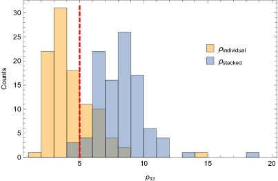
Figure 1: A histogram of the SNR of the 33-mode, $\rho_{33}$, from $100$ randomly sampled sets of detections, assuming a one year data acquisition time for aLIGO and uniform co-moving merger rate of $40\;{\rm Gpc}^{-3}{\rm yr}^{-1}$ Abbott et al. (2016d). We present the statistics of the largest $\rho_{33}$ event from each set (orange bins), and those with the stacked SNR using only the 15 largest SNR events from each set (blue bins). The 33-mode is detected if $\rho_{33}$ is above the detection threshold of $\rho_{33}=5$ (red dashed line). Refer to the main text for more details.

The resulting distribution (Fig. 1) indicates that there is roughly a $28\%$ chance for aLIGO to resolve at least one $33$-mode from a single event in one year of data at design sensitivity. After stacking, the probability of a collective 33-mode detection increases to $97\%$. These probabilities of course depend on the actual merger rate, as well as additional factors we have not taken into account here, including initial BH spins and precession. For example, if we take the more pessimistic event rate estimate of $13\;{\rm Gpc}^{-3}{\rm yr}^{-1}$ Abbott et al. (2016d), the probability for detection with a single event drops to $\sim 12\%$, while the collective mode detection probability drops to $50\%$ (still using 15 events).

In theory, all else being equal, coherent stacking should provide a $\sqrt{N}$ scaling of the SNR. Here $N=15$, so the ideal scenario would see a factor $\sim 3.8$ improvement in the collective $\rho_{33}$ relative to a single event. In our MC realizations we achieved improvement factors of between $1.3$ and $3.1$ relative to the loudest event over the set of 100 realizations (see the Supplemental Material for some additional comments and figures about the distribution). The primary reason for this is simply the non-uniform nature of the sampling, where it is typically the small handful of loudest events that contribute most to the collective SNR. The parameter uncertainty noise has smaller impact, in particular because the fainter events that have larger uncertainties are weighted less in the sum.

Discussion. We have presented a coherent mode stacking method that uses multiple high quality BBH coalescence detections to obtain better statistics for BH spectroscopy. Crucial to the method’s success is the appropriate alignment of the phase and frequency from different signals. For the class of BBH merger events we have targeted here, this is achievable for two primary reasons: (1) the no-hair properties of isolated BHs in GR imply that a binary system is likewise described by a small set of parameters, (2) the expected events that aLIGO will detect where the primary ringdown mode is visible will also have an inspiral detectable with high SNR, and this can be used to estimate the parameters in (1) with enough accuracy to predict the initial phases and amplitudes of sub-dominant ringdown modes. In this first, proof-of-principle study, we have demonstrated that detection of a collective secondary BH ringdown mode through stacking is likely with the current “advanced” generation of ground-based GW detectors, even if the corresponding modes are not loud enough to be detected in any single-event analysis.

There are many avenues for future work and extensions of this method, including using merger rates predicted by population synthesis models as done in Berti et al. (2016), considering other ringdown modes (such as the 44- and 21-modes Berti et al. (2016); Bhagwat et al. (2016), or even the fundamental 22-mode in a population of low SNR events where it is not individually detectable), adding spin to the progenitor BHs and also targeting secondary inspiral modes. Furthermore, this method could be adapted to constrain or search for other small-amplitude features that might be shared by a population of events, e.g. common parameterized post-Einsteinian-like Yunes and Pretorius (2009b) corrections to the inspiral phase of the mergers, or common equation-of-state-discriminating frequencies excited in hypermassive remnants of binary neutron star mergers Stergioulas et al. (2011); Takami et al. (2014, 2015); Bauswein et al. (2016); Bauswein and Stergioulas (2015); Paschalidis et al. (2015); East et al. (2016a, b); Lehner et al. (2016a); Radice et al. (2016); Lehner et al. (2016b). In this latter example, one issue in adapting the coherent stacking method would be achieving phase alignment, due to the challenge in accurately calculating the details of the matter dynamics post-merger. If the phases cannot be aligned, incoherent power stacking could still in theory achieve a $N^{1/4}$ SNR scaling (see Supplemental Material for more details).

Acknowledgements- HY thanks Haixing Miao for sharing the code for downhill simplex optimization. The authors thank Emanueli Berti, Swetha Bhagwat, Vitor Cardoso, Neil Cornish, Kendrick Smith, Chris Van Den Broeck and John Veitch for valuable discussions and comments. K.Y. acknowledges support from JSPS Postdoctoral Fellowships for Research Abroad. F.P. and V.P. acknowledge support from NSF grant PHY-1607449 and the Simons Foundation. V.P. also acknowledges support from NASA grant NNX16AR67G (Fermi). N.Y. acknowledges support from NSF CAREER Grant PHY-1250636. Computational resources were provided by XSEDE/TACC under grant TG-PHY100053. This research was supported in part by NSERC, and in part by the Perimeter Institute for Theoretical Physics. Research at Perimeter Institute is supported by the Government of Canada through the Department of Innovation, Science and Economic Development Canada, and by the Province of Ontario through the Ministry of Research and Innovation.

I Supplemental Material

I.1 Details in deriving the hypothesis test

The Generalized Likelihood Ratio Test (GLRT) was first presented in Shahram and Milanfar (2005) and applied to the ringdown analysis in Berti et al. (2007a) for single detection cases in the time domain, assuming white noise. Here we apply the same technique for the stacked signals we consider in this paper and we work in the frequency domain to account for the fact that detector noise is not white. We also include the effect of the parameter estimation noise due to the dominant mode subtraction in the analysis.

Let us start with the probability function (Eq. (7) in the main text)

$${\rm P}_{A} \propto {\rm exp}\left[-\int^{\infty}_{0}df\frac{2|\tilde{y}-A\tilde{\bf h}_{33}|^{2}}{S_{n}}\right]\,,$$ (10)

$$\propto \prod_{f>0}{\rm exp}\left[-\frac{2|\tilde{y}-A\tilde{\bf h}_{33}|^{2}}{S_{n}}\right]\,,$$

where the second line gives the discrete expression for ${\rm P}_{A}$ and the product $\prod$ is over different frequency bin contributions. By extremizing the likelihood, the maximum likelihood estimator for the amplitude is

$$\hat{A}= \frac{\langle{\bf h}_{33}|y\rangle}{\langle{\bf h}_{33}|{\bf h}_{33}\rangle}=\frac{1}{2}\frac{\int^{\infty}_{0}df\frac{\tilde{h}^{*}_{33}(f)\tilde{y}(f)+\tilde{h}_{33}(f)\tilde{y}^{*}(f)}{S_{n}(f)}}{\int_{0}^{\infty}df\frac{|\tilde{\bf h}_{33}|^{2}}{S_{n}}}\,,$$ (11)

with

$$\langle\chi|\xi\rangle\equiv 2\int^{\infty}_{0}\frac{\tilde{\chi}^{*}\tilde{\xi}+\tilde{\chi}\tilde{\xi}^{*}}{S_{n}}df.$$ (12)

In order to perform the GLRT test, we compute the following quantity

$$T(y)=\ln\frac{{\rm max}_{\mathcal{H}_{1}}P_{A}}{{\rm max}_{\mathcal{H}_{2}}P_{A=0}}=\frac{\hat{A}^{2}}{2}\langle{\bf h}_{33}|{\bf h}_{33}\rangle\,,$$ (13)

where in our specific situation, ${\rm max}_{\mathcal{H}_{1}}P_{A}=\max_{A}P_{A}$ and ${\rm max}_{\mathcal{H}_{2}}P_{A=0}=\max_{A}P_{A=0}=P_{A=0}$. Notice that since $P_{A=0}$ for hypothesis 2 does not depend on $A$, its maximization over $A$ simply gives $P_{A=0}$ itself. Assuming that the noise is Gaussian, $\sqrt{2T(y)}$ also follows a Gaussian distribution and one can propose that hypothesis $1$ is preferred if

$$\sqrt{2T(y)}=\frac{\langle{\bf h}_{33}|y\rangle}{\sqrt{\langle{\bf h}_{33}|{\bf h}_{33}\rangle}}=\frac{\langle{\bf h}_{33}|y\rangle}{||{\bf h}_{33}||}>\Gamma_{1}\,.$$ (14)

Here, $\Gamma_{1}$ is defined as $\Gamma_{\sigma^{2}}$ with the variance $\sigma^{2}=1$, where $\Gamma_{\sigma^{2}}$ is given by the false-alarm rate $P_{f}$: $\Gamma_{\sigma^{2}}=Q_{\sigma^{2}}^{-1}(P_{f})$ with $Q_{\sigma^{2}}(x)$ representing the right-tail probability function for a Gaussian distribution with zero mean and variance $\sigma^{2}$:

$$Q_{\sigma^{2}}(x)\equiv\frac{1}{\sqrt{2\pi}\sigma}\int^{\infty}_{x}e^{-\frac{z^{2}}{2\sigma^{2}}}dz\,.$$ (15)

The noise component of Eq. (14) is a normalized Gaussian distribution with zero mean and unit variance, with the latter explicitly given by

$${\rm Var}\left[\frac{\langle{\bf h}_{33}|{\bf n}\rangle}{||{\bf h}_{33}||}\right] =\left\langle\left(\frac{\langle{\bf h}_{33}|{\bf n}\rangle}{||{\bf h}_{33}||}\right)^{2}\right\rangle-\left\langle\frac{\langle{\bf h}_{33}|{\bf n}\rangle}{||{\bf h}_{33}||}\right\rangle^{2}$$

$$=\left\langle\frac{4}{||{\bf h}_{33}||^{2}}\int^{\infty}_{0}\int^{\infty}_{0}dfdf^{\prime}(\tilde{\bf h}^{*}_{33}(f)\tilde{n}(f)+h.c.)(\tilde{\bf h}^{*}_{33}(f^{\prime})\tilde{n}(f^{\prime})+h.c.)\frac{1}{S_{n}(f)S_{n}(f^{\prime})}\right\rangle$$

$$=\frac{4}{||{\bf h}_{33}||^{2}}\int^{\infty}_{0}df\frac{|\tilde{\bf h}_{33}(f)|^{2}}{S_{n}(f)}=1\,.$$ (16)

Here we used

$$\langle n(f)\rangle =0,$$ (17)

$$\langle n(f)n(f^{\prime})\rangle =0,$$ (18)

$$\langle n(f)n^{*}(f^{\prime})\rangle =\frac{1}{2}S_{n}(f)\delta(f-f^{\prime})\,,$$ (19)

for one-sided spectrum $S_{n}$ with $\langle X\rangle$ representing the expectation value of $X$, and the averaging operation $\langle\rangle$ is defined over an ensemble of noise realizations.

At this point, we notice that we only know the maximum likelihood estimator $y^{\prime}$ instead of $y$ (recall $y^{\prime}=y+\delta y)$ . In particular  ,

$$\sqrt{2T(y^{\prime})} \approx\frac{\langle{{\bf h}}^{\prime}_{33}|A{{\bf h}}_{33}+{\bf n}-n_{h_{22}}+An_{h_{33}}\rangle}{||{{\bf h}}^{\prime}_{33}||}$$

$$=A||{{\bf h}}_{33}+n_{h_{33}}||+\frac{\langle{{\bf h}}_{33}+n_{h_{33}}|{\bf n}-n_{h_{22}}\rangle}{||{{\bf h}}_{33}+n_{h_{33}}||}\,,$$ (20)

where the parameter uncertainty noise $n_{h_{\ell m}}$ is defined above Eq. (Black hole spectroscopy with coherent mode stacking). Let us further assume that noise is small and keep up to its second order. Neglecting cross terms such as $n_{h_{33}}{\bf n}$ and $n_{h_{33}}n_{h_{22}}$, where the former term has zero mean and the latter term is small due to the separation of resonance for $22$ and $33$ mode, the above equation becomes

$$\sqrt{2T(y^{\prime})} =A||{{\bf h}}_{33}||+A\frac{\langle{{\bf h}}_{33}|n_{h_{33}}\rangle}{||{{\bf h}}_{33}||}+\frac{A}{2}\frac{\langle n_{h_{33}}|n_{h_{33}}\rangle}{||{{\bf h}}_{33}||}$$

$$-\frac{A}{2}\frac{\langle{{\bf h}}_{33}|n_{h_{33}}\rangle^{2}}{||{{\bf h}}_{33}||^{3}}+\frac{\langle{{\bf h}}_{33}|{\bf n}-n_{h_{22}}\rangle}{||{{\bf h}}_{33}||}+\mathcal{O}(n^{3})\,.$$ (21)

Let us now derive a criterion for hypothesis 1 to pass the GLRT test including the parameter estimation noise. In the following, we use a bar to denote quantities for hypothesis 2 (not to be confused with the averaging operator $\langle\rangle$) while unbarred quantities refer to those for hypothesis 1. To $\mathcal{O}(\delta^{2})$, the distribution of $\sqrt{2T(y^{\prime})}$ for hypothesis 2 ($A=0$) has mean

$$\bar{\mu}=-\frac{\langle{{\bf h}}_{33}|\langle n_{h_{22}}\rangle\rangle}{||{{\bf h}}_{33}||}\,,$$ (22)

and variance

$${\rm Var}\left[\frac{\langle{\bf h}_{33}|{\bf n}-n_{h_{22}}\rangle}{||{\bf h}_{33}||}\right]$$

$$=1+{\rm Var}\left[\frac{\langle{\bf h}_{33}|n_{h_{22}}\rangle}{||{\bf h}_{33}||}\right]\equiv 1+\bar{\sigma}^{2}_{\rm p}\,,$$ (23)

where we neglect the correlation between ${\bf n}$ and $n_{h_{22}}$. Let us next shift the distribution by $-\bar{\mu}$ such that the shifted distribution has zero mean and denote the right-tail probability of the shifted distribution above $x$ as $\bar{Q}(x)$.

Although the distribution is not a Gaussian due to $\mathcal{O}(\delta^{2})$ terms in $\sqrt{2T(y^{\prime})}$, we next show that only the Gaussian part of $\bar{Q}(x)$ contributes to $\bar{\Gamma}\equiv\bar{Q}^{-1}(P_{f})$. We start by noting that $\bar{Q}$ is the right-tail probability of $\langle{\bf h}_{33}|{\bf n}\rangle/||{{\bf h}}_{33}||-\langle{\bf h}_{33}|n_{h_{22}}\rangle/||{{\bf h}}_{33}||+\bar{\mu}$. The first and second terms are Gaussian noise to $\mathcal{O}(\delta)$ so that the sum is also Gaussian to that order, with variance being $1+\bar{\sigma}^{2}_{\rm p}$ and $\bar{\Gamma}=\Gamma_{1}\sqrt{1+\bar{\sigma}^{2}_{\rm p}}$. Therefore the presence of $\mathcal{O}(\delta)$ noise component shifts $\Gamma_{1}$ by $\mathcal{O}(\delta^{2})$ order. Because the non-Gaussian noise component in $\sqrt{2T(y^{\prime})}$ enters at $\mathcal{O}(\delta^{2})$, its effect on $\bar{\Gamma}$ is at least on $\mathcal{O}(\delta^{3})$, which is beyond the order of perturbation we are considering. We conclude that we only need to consider the Gaussian contribution in $\bar{Q}$ to derive $\bar{\Gamma}$ valid to $\mathcal{O}(\delta^{2})$.

Thus, to the perturbation order we are working, it suffices to assume that the shifted distribution is a Gaussian given by $\bar{Q}=Q_{1+\bar{\sigma}^{2}_{\rm p}}$. Having such $\bar{Q}$ at hand, the criterion for hypothesis 1 to be preferred over hypothesis 2 for a given $y^{\prime}$ and $P_{f}$ given in Eq. (14) is modified to

$$\sqrt{2T(y^{\prime})}>\bar{Q}^{-1}(P_{f})=\Gamma_{1+\bar{\sigma}_{\rm p}^{2}}\,,$$ (24)

where $\Gamma_{1+\bar{\sigma}_{\rm p}^{2}}$ is equivalent to $\bar{\Gamma}$ in Eq. (I.1).

On the other hand, the distribution of $\sqrt{2T(y^{\prime})}$ for hypothesis 1 with $A=1$ to $\mathcal{O}(\delta^{2})$ has mean

$$\mu =||{\bf h}_{33}||+\frac{\langle{{\bf h}}_{33}|\langle n_{h_{33}}\rangle\rangle}{||{{\bf h}}_{33}||}+\frac{1}{2}\left\langle\frac{\langle n_{h_{33}}|n_{h_{33}}\rangle}{||{{\bf h}}_{33}||}\right\rangle$$

$$-\frac{1}{2}\left\langle\frac{\langle{{\bf h}}_{33}|n_{h_{33}}\rangle^{2}}{||{{\bf h}}_{33}||^{3}}\right\rangle$$

$$=||{\bf H}_{33}||+\bar{\mu}\,,$$ (25)

and variance

$${\rm Var}\left[\frac{\langle{\bf h}_{33}|{\bf n}-n_{h_{22}}+n_{h_{33}}\rangle}{||{\bf h}_{33}||}\right]$$

$$=1+{\rm Var}\left[\frac{\langle{\bf h}_{33}|n_{h_{22}}-n_{h_{33}}\rangle}{||{\bf h}_{33}||}\right]\equiv 1+\sigma^{2}_{\rm p}\,,$$ (26)

where ${\bf H}_{33}$ corresponds to the reduced 33 mode signal due to parameter uncertainties and is given by

$${\bf H}_{33} =\langle{\bf h}_{33}\rangle+\frac{1}{2}\left(\left\langle\frac{\langle n_{h_{33}}|n_{h_{33}}\rangle}{\langle{{\bf h}}_{33}|{{\bf h}}_{33}\rangle}\right\rangle-\left\langle\frac{\langle{{\bf h}}_{33}|n_{h_{33}}\rangle^{2}}{\langle{{\bf h}}_{33}|{{\bf h}}_{33}\rangle^{2}}\right\rangle\right){\bf h}_{33}$$

$$=\left[1+\frac{1}{2}\left(\left\langle\frac{\langle n_{h_{33}}|n_{h_{33}}\rangle}{\langle{{\bf h}}_{33}|{{\bf h}}_{33}\rangle}\right\rangle-\left\langle\frac{\langle{{\bf h}}_{33}|n_{h_{33}}\rangle^{2}}{\langle{{\bf h}}_{33}|{{\bf h}}_{33}\rangle^{2}}\right\rangle\right)\right]\langle{\bf h}_{33}\rangle$$

$$+\mathcal{O}(\delta^{3})\,,$$ (27)

with

$$\langle{\bf h}_{33}\rangle =e^{i(\omega_{33}t-\phi_{33})}\sum_{j}{\bf A}_{33,j}e^{-\Gamma_{33,j}t-(\sigma_{\Lambda_{33,j}}t)^{2}/2-(\sigma_{\Phi_{33,j}})^{2}/2}$$

$$+\mathcal{O}(\delta^{3})\,.$$ (28)

Here we used $\langle e^{x}\rangle=e^{\sigma_{x}^{2}/2}$ with the variance $\sigma_{x}^{2}\equiv\langle x^{2}\rangle$ for any complex Gaussian random variable $x$. Following the case for hypothesis 2, we shift the distribution by $-\mu$ such that its mean becomes zero. Then, the right-tail probability of the shifted distribution is simply given by $Q_{1+\sigma_{p}^{2}}$. Notice that the non-Gaussian contribution can be neglected as we discussed in the hypothesis 2 case.

To claim a detection of the 33 mode, we require that Eq. (24) be satisfied with the detection rate $P_{d}$. The criterion is given by

$$P_{d}\leq Q_{1+\sigma_{p}^{2}}\left(\Gamma_{1+\bar{\sigma}_{\rm p}^{2}}-\mu+\bar{\mu}\right)\,.$$ (29)

Using further the relation $Q_{\sigma^{2}}(x)=Q_{1}(x/\sigma)$, the above equation reduces to

$$\frac{||{\bf H}_{33}||}{\sqrt{1+\sigma_{p}^{2}}}\geq\frac{\Gamma_{1+\bar{\sigma}_{\rm p}^{2}}}{\sqrt{1+\sigma_{p}^{2}}}-Q_{1}^{-1}(P_{d})\,.$$ (30)

The left and right hand side of this inequality correspond to the SNR of the 33 mode including parameter uncertainties and the critical SNR for detection respectively. To simplify the latter further, we choose to be more conservative and replace $\Gamma_{1+\bar{\sigma}_{\rm p}^{2}}$ with $\Gamma_{1+\sigma_{\rm p}^{2}}(\geq\Gamma_{1+\bar{\sigma}_{\rm p}^{2}})$:

$$\rho_{33}\equiv\frac{||{\bf H}_{33}||}{\sqrt{1+\sigma^{2}_{\rm p}}}\geq Q_{1}^{-1}(P_{f})-Q_{1}^{-1}(P_{d})\equiv\rho_{\rm crit}\,,$$ (31)

where we used $\Gamma_{\sigma^{2}}=\sigma\Gamma_{1}$.

I.2 Estimating uncertainties in target mode phase

Of all the parameters considered in this work, the accuracy in estimating the constant phase offsets $\phi_{33,j}$ is the most important in improving the collective SNR. Here, we discuss in more detail the two dominant sources of error in this quantity.

The first comes from uncertainties in the intrinsic parameters estimated from each event, including the masses and spins of the individual BHs prior to merger. We estimate this effect in the following way. First, we employ full inspiral-merger-ringdown waveforms obtained with a numerical relativity surrogate model Blackman et al. (2015, 2017) with which we produce different waveforms to measure the individual total phases $\bm{\Phi\mkern-11.0mu\Phi}_{33}\equiv\omega_{33}t+\phi_{33}$ and $\bm{\Phi\mkern-11.0mu\Phi}_{22}\equiv\omega_{33}t+\phi_{22}$. Next, we time-shift the signals so that $t=0$ corresponds to the maximum amplitude of the GW. The difference between these phases is shown at the top plot of Fig. 2 for representative values of the mass ratio in binaries. Notice then that at $t=0$ one has a measure of $\phi_{33}$ relative to $\phi_{22}$. (Also, since the instance at which $t=0$ is chosen and the onset of the QNM is not sharply defined, we show the phases within a time-window around the peak in GW amplitude). To assess how this phase difference changes for different BH masses and spins, we vary these values within the uncertainties reported for GW150914 and plot the difference $\bm{\Delta}\bm{\Phi\mkern-11.0mu\Phi}_{33-22}$ in the middle and bottom panels of Fig. 2 .

An additional possible source of uncertainty in $\phi_{33,j}$ is due to uncertainties in the polarization and inclination angles of the source (relative to the line of sight), as the dependence of $\phi_{33,j}$ on the polarization phase can be different among different $\ell$ modes. However, such uncertainties are of order $\sim 1\%$. This can be seen by noticing that in a spin-weighted spherical harmonic decomposition no differences arise Klein et al. (2009) and the transformation to the required spin-weighted spheroidal harmonic introduce such small effect Berti et al. (2006b, 2007a); Berti and Klein (2014). Thus, this source of uncertainty is negligible in our analysis.

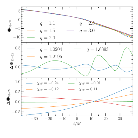
Figure 2: Top panel: difference between the total phase of the 33 mode and that of the 22 mode, i.e., $\bm{\Phi\mkern-11.0mu\Phi}_{33-22}=\bm{\Phi\mkern-11.0mu\Phi}_{33}-\bm{\Phi\mkern-11.0mu\Phi}_{22}$ for different mass ratios. Middle/Bottom panel: variation of $\bm{\Phi\mkern-11.0mu\Phi}_{33-22}$ using the expected mean parameters of ${\rm GW150914}$ and expected mass ratio/effective spin uncertainties of ${\rm GW150914}$ Abbott et al. (2016e) (to $90\%$ credible levels) . Here the spins of both black holes are assumed to be aligned and equal (other spin combinations within the confidence interval of $\chi_{\rm eff}$ give similar variations).

Based on the above considerations, we estimate $\sigma_{\Phi_{33}}=0.3\times(20/\rho)$ rads, where the value of 0.3 rads for $\rho=20$ is extracted from the middle and bottom panels of Fig. 2 with $t\in(0,10)M$, within which we expect the onset of the ringdown phase. While this estimate is obtained from GW$150914$, we anticipate that generally BH binaries could have very different spin configurations. Understanding the spin dependence of phase errors is necessary for more systematic future studies. The $1/\rho$ scaling can be obtained through a straightforward Fisher analysis and error propagation as follows: Using an IMR waveform, we estimate the covariance matrix $\Sigma_{ab}^{\mathrm{(insp)}}$ of the inspiral parameters (individual masses and spins) $\theta^{a}_{\mathrm{(insp)}}$ as the inverse of the Fisher matrix. Since $\theta^{a}_{\mathrm{(insp)}}$ are related to the ringdown parameters $\theta^{a}_{\mathrm{(rd)}}=(A_{\ell m},\Omega_{\ell m},\Gamma_{\ell m},\Phi_{\ell m})$, we approximately obtain the covariance matrix of the latter as

$$\Sigma_{ab}^{\mathrm{(rd)}}=\sum_{p,q}\frac{\partial\theta^{a}_{\mathrm{(rd)}}}{\partial\theta^{p}_{\mathrm{(insp)}}}\frac{\partial\theta^{b}_{\mathrm{(rd)}}}{\partial\theta^{q}_{\mathrm{(insp)}}}\Sigma_{pq}^{\mathrm{(insp)}}\,.$$ (32)

Since $\Sigma_{ab}^{\mathrm{(insp)}}$ is proportional to $1/\rho^{2}$, the uncertainty in $\theta^{a}_{\mathrm{(rd)}}$ (equivalent to $\sqrt{\Sigma_{aa}^{\mathrm{(rd)}}}$) scales as $1/\rho$. One can also use the previous formula to estimate the amount of correlation among the ringdown parameters.

I.3 Monte-Carlo sampling, comparison to earlier single-rate estimates, and SNR boost through stacking

Here we provide some additional comments and details regarding our Monte-Carlo sampling of simulated events, illustrated in Fig. 1 in the main text, and Fig. 3 below.

First, our estimate of a 0.3/yr detection rate for the 33-mode without the coherent mode stacking implied in Fig. 1 is larger than the $\sim 0.03$/yr rate predicted in Berti et al. (2016). One of the reasons for this difference arises from the value of $A_{33}/A_{22}$ we have used. Here we employ the fitting formula derived in London et al. (2014), which typically gives a ratio 1.6 times larger than that used in the earlier study. The difference between the ratios from these fitting formulas is mostly related to the choice of “starting time” of QNMs. Had we instead used the ratio as in Berti et al. (2007a, 2016), it would have effectively raised $\rho_{\mathrm{crit}}$ to $4.65\times 1.6\sim 7.5$, dropping the expected event rate of the 33-mode to $\sim 0.06$/yr (see Fig. 1). The second reason for our higher rate comes from the larger merger rate of $40{\rm Gpc}^{-3}{\rm yr}^{-1}$ Abbott et al. (2016d) that we use. These two factors together make our single-event rate estimate consistent with Berti et al. (2016).

As mentioned in the main text, the reason we do not get prefect $\sqrt{N}$ scaling when stacking is due to the non-uniform distribution of SNRs. In a typical sample, the individual SNRs have a pyramid-like distribution (as indicated in Fig. 3), and the top few loudest events matter the most enhancing the collective vs. single-loudest event SNR. This is also why increasing the number of events used beyond the $N=15$ chosen here will not significantly increase the stacked SNR, and we could probably have used even fewer than $15$ without much degradation of the SNR. The value of $15$ was chosen simply to reduce the computational cost of the simulations, and we leave it to future work to find an adequate $N$ giving most of the SNR with least computational cost.

For illustrative purposes, in Fig. 4 we show that if we did have a set of identical sources we would obtain $\sqrt{N}$ scaling in the stacking process. There, we took $15$ events that are identical to GW$150914$, all with the same noise spectrum, and then stacked them coherently as discussed in the main text. In the figure we show the original signal, detector noise (assuming aLIGO noise) versus the stacked signal and stacked detector noise.

A relatively minor factor in reducing the efficacy of stacking can be attributed to the frequency rescaling of the noise spectrum $S_{n}$. Because the detector noise curve is not flat in frequency, overlapping rescaled noise spectra can add low-sensitivity regions to high-sensitivity ones, leading to worse overall noise performance when compared to the case where no rescaling is required. This could be mitigated to some extent by a judicial choice of the particular target-mode frequency we choose to scale all events to; we leave that to future work to investigate.

A final adverse affect on the stacked SNR we note is due to parameter estimation noise; we estimate it reduces the final SNR by $\sim 5\%$ in a typical MC simulation set. If future parameter uncertainty studies suggest larger phase errors (for example, imagine spin effects to be very different from GW$150914$), a more conservative estimate with $\sigma_{\Phi_{33}}=0.6\times(20/\rho)$ rad (twice as we have assumed in the main text) reduces the final SNR by $\sim 15\%$.

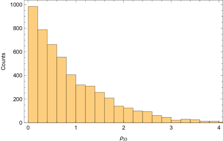
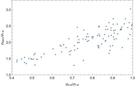
Figure 3: (Left) A collection of all events in $100$ sets of data, showing the distribution of individual 33-mode SNR. The tail of the distribution does contain events with $\rho_{33}>4$ (see Fig. 1), though here we focus on the dominant range of the distribution. (Right) Scatter plot of the $100$ sets of data, with the horizontal axis being the ratio of $\rho_{33}$ between the second loudest and loudest event within each set, and the vertical axis being the ratio between the SNR of the stacked signal and that of the loudest event. Observe that the coherent mode stacking works more efficiently when the SNR of the loudest event is closer to that of the second largest event.

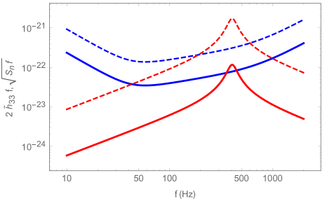
Figure 4: Detector noise (thick blue), stacked noise (dashed blue) v.s. signal (thick red) and the stacked signal (dashed red), assuming $15$ ${\rm GW150914}$-like events with aLIGO sensitivity. For comparison purposes, we have rescaled the noise component and signal component so that they are both dimensionless. In particular, the noise is rescaled as $\sqrt{S_{n}f}$ and the signal is rescaled as $2f\tilde{h}_{33}$. The stacked detector noise is $\sqrt{15}$ times larger than the noise of a single detector and the stacked signal is 15 times larger than the original signal.

I.4 Power stacking

For completeness, we note an alternative approach to stacking signals in the hypothesis test set-up Meidam et al. (2014). Assuming one does not have prior information about the phase of the $33$-mode, one can multiply the probability function (or Bayes factors) of single detections to obtain the total probability function

$$P_{A}\propto\prod_{j}\prod_{f>0}\exp\left[-\frac{2|\tilde{y}_{j}-A_{j}\tilde{h}_{33,j}|^{2}}{S_{n_{j}}}\right]\,,$$ (33)

where $j$ labels the individual detections. Each event has its own maximum likelihood estimator as given in the single detection case. The generalized likelihood ratio test suggests

$$T(y_{j},j=1\ldots N) =\ln\frac{{\rm max}_{H_{1}}P_{A}}{{\rm max}_{H_{2}}P_{A=0}}$$

$$=\sum^{N}_{j=1}\frac{\hat{A}_{j}^{2}}{2}\langle h_{33,j}|h_{33,j}\rangle\,.$$ (34)

It is straightforward to see that the noise part of $T$ follows a $\chi^{2}_{N}$ distribution, which we label as $R$ here. We say hypothesis $1$ is preferred if

$$P_{d}\leq R\left(R^{-1}(P_{f})-\sum^{N}_{j=1}A_{j}^{2}\langle h_{33,j}|h_{33,j}\rangle\right)\,,$$ (35)

or equivalently

$$\sum^{N}_{j=1}A_{j}^{2}\langle h_{33,j}|h_{33,j}\rangle\geq R^{-1}(P_{f})-R^{-1}(P_{d})\,.$$ (36)

Let us assume that we are looking at events all with the same SNR. When $N$ is large, the $\chi^{2}_{N}$ distribution can be well approximated by a Gaussian distribution, so that the right hand side of the above equation scales as $\sqrt{N}$. On the other hand, the left hand side of the equation scales as $N$. As a result, the improvement due to this stacking process is equivalent to lowering $S_{n}$ (which comes from $\langle h_{33,j}|h_{33,j}\rangle$) by a factor $\sqrt{N}$, or the “amplitude” of noise (characterized by $\sqrt{S_{n}}$) by a factor of $N^{1/4}$. Therefore this power stacking process improves the SNR with a suboptimal $\mathcal{O}(N^{1/4})$ when $N$ is large but, as described, does not require phase knowledge. Such a scaling in SNR is consistent with that in e.g. Kalmus et al. (2009).

We now compare the previous calculations of power stacking and coherent stacking with a Bayesian model selection study with multiple events performed in Meidam et al. (2014). In this reference, the authors construct an odds ratio of multiple events by multiplying the Bayes factor of each event. This gives a factor of $N$ improvement on the odds ratio compared to a single event case, just like the log of the maximum likelihood ratio $T(y_{j})$ in Eq. (I.4) improves by the same factor. One then needs to compare the odds ratio with a threshold to determine which hypothesis is preferred. Since the threshold on the right hand side of Eq. (36) scales with $\sqrt{N}$, we expect that the same scaling holds for the threshold of the odds ratio. Thus, $\rho^{2}$ scales with $N/\sqrt{N}=\sqrt{N}$ in this case. On the other hand, if one uses the coherent mode stacking, $T(y)$ in Eq. (13) also scales with a factor of $N$ but the threshold (corresponding to $\Gamma^{2}/2$ from Eq. (14)) is independent of $N$. Thus, $\rho^{2}$ scales with $N$ in the coherent mode stacking case. This is why the coherent mode stacking should have an advantage over the power stacking, but at the price of using full waveform information.

At this stage, we recall that if we know the exact phase and frequency of $33$ modes in each detection a priori, or if we are performing parameter estimation for a universal parameter (let’s say $A$), we can replace all $A_{j}$’s in Eq. (33) by a single parameter $A$ and perform the GLRT again. In this case, a straightforward calculation shows that we gain order $\sqrt{N}$ in SNR using Bayesian approach. Of course in reality the phase and frequency of $33$ modes are never known perfectly, but one can imagine that an improved Bayesian approach, for example using the Bayesian model selection with a combined odds ratio in Meidam et al. (2014) and taking into account prior information with parameter uncertainties, should give consistent result with the coherent mode stacking method discussed here. In other words, it is likely that the full waveform information can be folded into a Bayesian model selection in which case the improvement should be comparable to the coherent stacking method.

References

- Abbott et al. (2016a) B. P. Abbott et al. (Virgo, LIGO Scientific), Phys. Rev. Lett. 116, 061102 (2016a), eprint 1602.03837.
- Abbott et al. (2016b) B. P. Abbott et al. (Virgo, LIGO Scientific), Phys. Rev. Lett. 116, 241103 (2016b), eprint 1606.04855.
- Yunes and Siemens (2013) N. Yunes and X. Siemens, Living Reviews in Relativity 16 (2013), eprint 1304.3473, URL http://www.livingreviews.org/lrr-2013-9.
- Abbott et al. (2016c) B. P. Abbott et al. (Virgo, LIGO Scientific), Phys. Rev. Lett. 116, 221101 (2016c), eprint 1602.03841.
- Yunes et al. (2016) N. Yunes, K. Yagi, and F. Pretorius, Phys. Rev. D94, 084002 (2016), eprint 1603.08955.
- Abbott et al. (2016d) B. P. Abbott et al. (Virgo, LIGO Scientific), Phys. Rev. X6, 041015 (2016d), eprint 1606.04856.
- Lasky et al. (2016) P. D. Lasky, E. Thrane, Y. Levin, J. Blackman, and Y. Chen, arXiv preprint arXiv:1605.01415 (2016).
- Israel (1967) W. Israel, Phys. Rev. 164, 1776 (1967).
- Carter (1971) B. Carter, Physical Review Letters 26, 331 (1971).
- Hawking (1972) S. W. Hawking, Commun. Math. Phys. 25, 152 (1972).
- Robinson (1975) D. C. Robinson, Physical Review Letters 34, 905 (1975).
- Cardoso and Gualtieri (2016) V. Cardoso and L. Gualtieri, Classical and Quantum Gravity 33, 174001 (2016).
- Dreyer et al. (2004) O. Dreyer, B. J. Kelly, B. Krishnan, L. S. Finn, D. Garrison, and R. Lopez-Aleman, Class. Quant. Grav. 21, 787 (2004), eprint gr-qc/0309007.
- Berti et al. (2006a) E. Berti, V. Cardoso, and C. M. Will, Phys. Rev. D73, 064030 (2006a), eprint gr-qc/0512160.
- Kamaretsos et al. (2012) I. Kamaretsos, M. Hannam, S. Husa, and B. S. Sathyaprakash, Phys. Rev. D85, 024018 (2012), eprint 1107.0854.
- Gossan et al. (2012) S. Gossan, J. Veitch, and B. S. Sathyaprakash, Phys. Rev. D85, 124056 (2012), eprint 1111.5819.
- Jackiw and Pi (2003) R. Jackiw and S. Y. Pi, Phys. Rev. D68, 104012 (2003), eprint gr-qc/0308071.
- Alexander and Yunes (2009) S. Alexander and N. Yunes, Phys. Rept. 480, 1 (2009), eprint 0907.2562.
- Yunes and Pretorius (2009a) N. Yunes and F. Pretorius, Phys. Rev. D79, 084043 (2009a), eprint 0902.4669.
- Yagi et al. (2012) K. Yagi, N. Yunes, and T. Tanaka, Phys.Rev. D86, 044037 (2012), eprint 1206.6130.
- Campbell et al. (1992) B. A. Campbell, N. Kaloper, and K. A. Olive, Physics Letters B 285, 199 (1992).
- Kanti et al. (1996) P. Kanti, N. Mavromatos, J. Rizos, K. Tamvakis, and E. Winstanley, Phys.Rev. D54, 5049 (1996), eprint hep-th/9511071.
- Yunes and Stein (2011) N. Yunes and L. C. Stein, Phys. Rev. D83, 104002 (2011), eprint 1101.2921.
- Pani and Cardoso (2009) P. Pani and V. Cardoso, Phys.Rev. D79, 084031 (2009), eprint 0902.1569.
- Yunes and Stein (2011) N. Yunes and L. C. Stein, Phys. Rev. D 83, 104002 (2011), eprint 1101.2921.
- Pani et al. (2011) P. Pani, C. F. B. Macedo, L. C. B. Crispino, and V. Cardoso, Phys. Rev. D84, 087501 (2011), eprint 1109.3996.
- Ayzenberg and Yunes (2014) D. Ayzenberg and N. Yunes, Phys. Rev. D90, 044066 (2014), [Erratum: Phys. Rev.D91,no.6,069905(2015)], eprint 1405.2133.
- Brito et al. (2013) R. Brito, V. Cardoso, and P. Pani, Phys. Rev. D88, 064006 (2013), eprint 1309.0818.
- Berti et al. (2016) E. Berti, A. Sesana, E. Barausse, V. Cardoso, and K. Belczynski, Phys. Rev. Lett. 117, 101102 (2016), eprint 1605.09286.
- Bhagwat et al. (2016) S. Bhagwat, D. A. Brown, and S. W. Ballmer, Phys. Rev. D94, 084024 (2016), eprint 1607.07845.
- Berti et al. (2007a) E. Berti, J. Cardoso, V. Cardoso, and M. Cavaglia, Phys. Rev. D76, 104044 (2007a), eprint 0707.1202.
- Meidam et al. (2014) J. Meidam, M. Agathos, C. Van Den Broeck, J. Veitch, and B. S. Sathyaprakash, Phys. Rev. D90, 064009 (2014), eprint 1406.3201.
- London et al. (2014) L. London, D. Shoemaker, and J. Healy, Phys. Rev. D90, 124032 (2014), [Erratum: Phys. Rev.D94,no.6,069902(2016)], eprint 1404.3197.
- Buonanno et al. (2007) A. Buonanno, G. B. Cook, and F. Pretorius, Phys. Rev. D 75, 124018 (2007), URL http://link.aps.org/doi/10.1103/PhysRevD.75.124018.
- Berti et al. (2007b) E. Berti, V. Cardoso, J. A. Gonzalez, U. Sperhake, M. Hannam, S. Husa, and B. Brügmann, Phys. Rev. D 76, 064034 (2007b), URL http://link.aps.org/doi/10.1103/PhysRevD.76.064034.
- Yang et al. (2012) H. Yang, D. A. Nichols, F. Zhang, A. Zimmerman, Z. Zhang, and Y. Chen, Phys. Rev. D 86, 104006 (2012), URL http://link.aps.org/doi/10.1103/PhysRevD.86.104006.
- Husa et al. (2016) S. Husa, S. Khan, M. Hannam, M. Purrer, F. Ohme, X. J. Forteza, and A. Bohe, Phys. Rev. D93, 044006 (2016), [Phys. Rev.D93,044006(2016)], eprint 1508.07250.
- Ajith et al. (2011) P. Ajith et al., Phys. Rev. Lett. 106, 241101 (2011), eprint 0909.2867.
- Ajith (2011) P. Ajith, Phys. Rev. D84, 084037 (2011), eprint 1107.1267.
- Nelder and Mead (1965) J. A. Nelder and R. J. Mead, The Computer Journal 7, 308 (1965).
- Press et al. (2007) W. H. Press, B. P. Flannery, S. A. Teukolsky, and W. T. Vetterling, Numerical Recipes: The Art of Scientific Computing (Cambridge University Press, Cambridge (UK) and New York, 2007).
- Yunes and Pretorius (2009b) N. Yunes and F. Pretorius, Phys.Rev. D80, 122003 (2009b), eprint 0909.3328.
- Stergioulas et al. (2011) N. Stergioulas, A. Bauswein, K. Zagkouris, and H.-T. Janka, Mon. Not. Roy. Astron. Soc. 418, 427 (2011), eprint 1105.0368.
- Takami et al. (2014) K. Takami, L. Rezzolla, and L. Baiotti, Phys. Rev. Lett. 113, 091104 (2014), eprint 1403.5672.
- Takami et al. (2015) K. Takami, L. Rezzolla, and L. Baiotti, Phys. Rev. D91, 064001 (2015), eprint 1412.3240.
- Bauswein et al. (2016) A. Bauswein, N. Stergioulas, and H.-T. Janka, Eur. Phys. J. A52, 56 (2016), eprint 1508.05493.
- Bauswein and Stergioulas (2015) A. Bauswein and N. Stergioulas, Phys. Rev. D91, 124056 (2015), eprint 1502.03176.
- Paschalidis et al. (2015) V. Paschalidis, W. E. East, F. Pretorius, and S. L. Shapiro, Phys. Rev. D92, 121502 (2015), eprint 1510.03432.
- East et al. (2016a) W. E. East, V. Paschalidis, F. Pretorius, and S. L. Shapiro, Phys. Rev. D93, 024011 (2016a), eprint 1511.01093.
- East et al. (2016b) W. E. East, V. Paschalidis, and F. Pretorius (2016b), eprint 1609.00725.
- Lehner et al. (2016a) L. Lehner, S. L. Liebling, C. Palenzuela, O. L. Caballero, E. O’Connor, M. Anderson, and D. Neilsen, Class. Quant. Grav. 33, 184002 (2016a), eprint 1603.00501.
- Radice et al. (2016) D. Radice, S. Bernuzzi, and C. D. Ott, Phys. Rev. D94, 064011 (2016), eprint 1603.05726.
- Lehner et al. (2016b) L. Lehner, S. L. Liebling, C. Palenzuela, and P. M. Motl, Phys. Rev. D94, 043003 (2016b), eprint 1605.02369.
- Shahram and Milanfar (2005) M. Shahram and P. Milanfar, IEEE Transactions on Signal Processing 53, 2579 (2005).
- Blackman et al. (2015) J. Blackman, S. E. Field, C. R. Galley, B. Szil gyi, M. A. Scheel, M. Tiglio, and D. A. Hemberger, Phys. Rev. Lett. 115, 121102 (2015), eprint 1502.07758.
- Blackman et al. (2017) J. Blackman, S. E. Field, M. A. Scheel, C. R. Galley, D. A. Hemberger, P. Schmidt, and R. Smith (2017), eprint 1701.00550.
- Klein et al. (2009) A. Klein, P. Jetzer, and M. Sereno, Phys. Rev. D80, 064027 (2009), eprint 0907.3318.
- Berti et al. (2006b) E. Berti, V. Cardoso, and M. Casals, Phys. Rev. D73, 024013 (2006b), [Erratum: Phys. Rev.D73,109902(2006)], eprint gr-qc/0511111.
- Berti and Klein (2014) E. Berti and A. Klein, Phys. Rev. D 90, 064012 (2014), URL http://link.aps.org/doi/10.1103/PhysRevD.90.064012.
- Abbott et al. (2016e) B. P. Abbott, R. Abbott, T. D. Abbott, M. R. Abernathy, F. Acernese, K. Ackley, C. Adams, T. Adams, P. Addesso, R. X. Adhikari, et al. (LIGO Scientific Collaboration and Virgo Collaboration), Phys. Rev. Lett. 116, 241102 (2016e), URL http://link.aps.org/doi/10.1103/PhysRevLett.116.241102.
- Kalmus et al. (2009) P. Kalmus, K. C. Cannon, S. Marka, and B. J. Owen, Phys. Rev. D80, 042001 (2009), eprint 0904.4906.
- Barausse et al. (2014) E. Barausse, V. Cardoso, and P. Pani, Phys. Rev. D 89, 104059 (2014), URL http://link.aps.org/doi/10.1103/PhysRevD.89.104059.
- Nakano et al. (2015) H. Nakano, T. Tanaka, and T. Nakamura, Phys. Rev. D92, 064003 (2015), eprint 1506.00560.
- Veitch and Vecchio (2010) J. Veitch and A. Vecchio, Phys. Rev. D81, 062003 (2010), eprint 0911.3820.
- Etienne et al. (2008) Z. B. Etienne, J. A. Faber, Y. T. Liu, S. L. Shapiro, K. Taniguchi, and T. W. Baumgarte, Phys. Rev. D77, 084002 (2008), eprint 0712.2460.
- Gold et al. (2014) R. Gold, V. Paschalidis, M. Ruiz, S. L. Shapiro, Z. B. Etienne, and H. P. Pfeiffer, Phys. Rev. D90, 104030 (2014), eprint 1410.1543.