Abstract

We consider a minimal interacting theory of a single tower of spin $j=0,2,4,...$ massless Fronsdal fields in flat space with local Lorentz -covariant cubic interaction vertices. We address the question of constraints on possible quartic interaction vertices imposed by the condition of on-shell gauge invariance of the tree-level four-point scattering amplitudes involving three spin 0 and one spin $j$ particle. We find that these constraints admit a local solution for quartic $000j$ interaction term in the action only for $j=2$ and $j=4$. We determine the non-local terms in four-vertices required in the $j\geq 6$ case and suggest that these non-localities may be interpreted as a result of integrating out a tower of auxiliary ghost-like massless higher spin fields in an extended theory with a local action, up to possible higher-point interactions of the ghost fields. We also consider the conformal off-shell extension of the Einstein theory and show that the perturbative expansion of its action is the same as that of the non-local action resulting from integrating out the trace of the graviton field from the Einstein action. Motivated by this example, we conjecture the existence of a similar conformal off-shell extension of a massless higher spin theory that may be related to the above extended theory. It may then have the same infinite-dimensional symmetry as the higher-derivative conformal higher spin theory and may thus lead to a trivial S matrix.

Imperial-TP-AAT-2017-01

1 Introduction

The existence of an interacting theory of massless higher spins in flat space is usually considered to be problematic due to various no-go theorems (see [1]). While cubic higher spin interaction vertices consistent with on-shell gauge invariance were constructed in various approaches [2, 3, 4, 5, 6, 7, 8, 9] it is not a priori clear if they can be completed by quartic and higher vertices to a local gauge-invariant action that can be used to define non-trivial observables. These issues were addressed in [10, 11, 12] and recently in [13, 14, 15, 16, 17, 18].

Here we shall revisit the construction of quartic higher spin interaction vertices for a minimal theory of a single tower of massless even spins $j=0,2,4,...$ (without internal symmetry indices) using the Lorentz-covariant S-matrix-based approach. We shall assume that the theory should admit a Lorentz-covariant formulation with local on-shell gauge-invariant cubic vertices and determine the type of non-localities that may appear in the quartic vertices. We shall consider the tree amplitudes involving three scalar fields and one spin $j$ field and show that in the cases of $j=2$ and $j=4$ there exist local quartic $000j$ interaction terms in the action that render the amplitudes on-shell gauge invariant. However, for $j\geq 6$ we shall find that the gauge invariance requires the introduction of non-local four-point vertices in the action.

One may wonder if the locality can be restored by extending the set of fields. We will suggest that this may be possible by adding a second tower of even spin $j>0$ fields with specific couplings to the fields of the original set. There are indications that the resulting extended interacting action may still lead, after the summation over all intermediate higher spin exchanges, to a trivial S matrix. That would be in agreement with constraints imposed by gauge invariance (under the key assumption of locality) on massless higher spin scattering amplitudes that can be found in a soft momentum limit.

A related question is about an underlying global symmetry of such conjectured flat-space massless higher spin theory. While for the higher spin theory in AdS space there is a natural higher spin symmetry algebra [19], it is unclear a priori if it has a flat-space counterpart. By analogy with the Einstein theory that admits a conformal off shell extension [20] (found by introducing a conformally coupled scalar and then solving for it) one may conjecture that there exists a massless higher spin theory which is invariant under the same conformal higher spin algebra as the conformal higher spin theory [21, 22]. In contrast to the higher-derivative but local conformal higher spin action, the action of the minimal massless higher spin theory with two-derivative kinetic terms for a single tower of even spins should be non-local. Its infinite dimensional global symmetry may then be expected to constrain the S matrix to be trivial like in the conformal higher spin theory [23, 24]. That the scattering amplitudes of a massless higher spin theory in flat space should vanish as a consequence of a higher spin symmetry was also argued for in [16].

We shall start in section 2 by discussing the conditions that gauge invariance imposes on S-matrix elements, emphasizing that only the “linear” part of the gauge transformation (i.e. the part independent of the fields) constrains the S matrix. We will also review the Lorentz-covariant local three-point vertices we will start with and specify the general form of the quartic Lagrangian that will be relevant for the calculation of the $000j$ tree-level scattering amplitude.

In section 3 we will compute the tree-level $000j$ S-matrix element, finding separately the exchange part and the contribution of the quartic interaction term in the Lagrangian. We will then consider their gauge transformations and extract the constraints imposed by the gauge invariance of the total amplitude on the coefficient functions appearing in the quartic vertex.

Section 4 will contain the analysis of these constraints. For $j=2$ and $j=4$ we will find that there exist local quartic terms in the Lagrangian that are consistent with the gauge invariance of the amplitude, while for $j\geq 6$ a quartic Lagrangian must be nonlocal.

In section 5 we will present a “minimal” choice of nonlocal terms required by gauge invariance of the S matrix and suggest a way of eliminating the nonlocalities by introducing an additional tower of “ghost-like” higher spin fields. It turns out that the additional quartic nonlocal interaction of spin-0 particles required by this procedure is such that it cancels the exchange part of spin-0 four-particle amplitude. Further nonlocal non-minimal terms may completely cancel all the singular terms of the exchange part of the $000j$ amplitude.

In section 6 we will consider the conformal off-shell extension of the Einstein theory and show that its perturbative expansion is the same as that of the non-local action resulting from integrating out the trace of the graviton field from the standard Einstein Lagrangian. We will then conjecture the existence of a similar conformal off-shell extension of a massless higher spin theory that may have the same symmetries as the conformal higher spin theory.

Appendix A will contain some details of the the contribution of the quartic Lagrangian to the $000j$ amplitude and its organization into a basis of contractions of the spin-$j$ polarization tensor used in section 3.

In Appendix B we will place the results of sections 3–5 into a more general context by presenting the analysis of the constraints imposed by the on-shell gauge invariance and locality on generic massless higher spin scattering amplitudes $j_{1}\dots j_{n}j$. Similar analysis was performed earlier in [11] with the same conclusions. We shall use the soft momentum $p_{n+1}\to 0$ expansion generalizing the discussions in [25, 26, 27] to arbitrary couplings of higher-spin fields.

In Appendix C we will demonstrate that there exists a special choice of on-shell gauges (or, equivalently, reference vectors in polarization tensors) for which the non-local four-point vertex resulting from integrating out the trace of the graviton field in the Einstein action gives a vanishing contribution to the four-graviton amplitude.

2 Lagrangian vs. S-matrix gauge symmetries and
massless higher spin interaction vertices

The construction of Lagrangians invariant under gauge transformations can be done using the Noether procedure but this is typically difficult. In this section we will first argue that a more efficient and technically more straightforward approach is to start with the S matrix and demand its (on-shell) gauge invariance. We shall then review the known local Lorentz-covariant cubic interactions of massless higher-spin fields and write down the most general ansatz for the spin $000j$ quartic Lagrangian which will be used in the following sections.

2.1 Gauge transformations from the perspective of the S matrix

Lagrangians exhibiting gauge symmetries are usually determined through an iterative Noether procedure. One starts with a quadratic action and deforms it by higher-order terms while simultaneously deforming the linearized gauge transformations in such a way that the resulting action is invariant off-shell under the deformed transformations. This procedure links the construction of the full action $S=S_{2}+S_{3}+S_{4}+...$ to the determination of a non-linear modification of the gauge transformations $\delta=\delta^{(0)}+\delta^{(1)}+\delta^{(2)}+...$. For the cubic part of the action one is to solve the equation

$$\delta^{(0)}S_{3}+\delta^{(1)}S_{2}=0\ ,$$ (2.1)

where $\delta^{(1)}$ is a deformation of the gauge transformations linear in the fields. Thus, the cubic action must be invariant under the linearized gauge transformations up to the term proportional to the free equations of motion. The quartic action $S_{4}$ is then found from

$$\delta^{(0)}S_{4}+\delta^{(1)}S_{3}+\delta^{(2)}S_{2}=0\ .$$ (2.2)

Determining higher $\delta^{(n)}$ simultaneously with $S_{n+2}$ is not always straightforward, especially in theories with many fields.

An alternative approach is to constrain the Lagrangian by demanding that the tree-level scattering amplitudes following from it are invariant under the on-shell gauge transformations. The essential advantage of this approach is that only the linearized gauge transformations $\delta^{(0)}$ act on physical scattering amplitudes. While field-dependent (“nonlinear”) terms in the gauge transformation,

$$\delta\phi\sim\partial\epsilon+\phi\,\epsilon+\dots\ ,$$ (2.3)

relate $n$-point Green’s functions to Green’s functions of at least $n+1$ fields, such terms are projected out by the amputation relating the $n$-point Green’s functions and $n$-point scattering amplitudes at generic momenta. Indeed, for asymptotic states with momenta $p_{1},\dots,p_{n}$, the amputation leading to the $n$-point amplitude selects the most singular term proportional to $p_{1}^{-2}\dots p_{n}^{-2}$ by multiplication with $p_{1}^{2}\dots p_{n}^{2}$ and taking the on-shell limit $p_{i}^{2}=0$. For an $(n+r)$-point ($r=1,2,...$) Green’s function resulting from a nonlinear term in the gauge transformations the momentum conservation requires that it should have a different pole structure. Thus such terms are amputated away, i.e. all the nonlinear terms in the symmetry transformations applied to Green’s functions are projected out by the LSZ reduction.

In the context of the Yang-Mills theory this is reflected in that the amplitudes are invariant under the global part of the gauge group and vanish if the polarization vector of a gluon $\varepsilon_{\mu}(p)$ is replaced by the momentum

$$\delta^{(0)}A_{\mu}=\partial_{\mu}\epsilon~{}~{}\longrightarrow~{}~{}\delta\varepsilon_{\mu}(p)=p_{\mu}\,\epsilon(p)\ .$$ (2.4)

For massless higher-spin fields ($\phi_{s}\equiv\phi_{\mu_{1}\cdots\mu_{s}}$) the linearized gauge transformations are given by the first term in (2.3), i.e. symbolically

$$\delta^{(0)}\phi_{s}=\partial\epsilon_{s-1}\ .$$ (2.5)

The corresponding scattering amplitudes for any number of external legs and loop order should thus be invariant under the following transformation of the polarisation tensor $\phi_{\mu_{1}\cdots\mu_{s}}(p)$ (in momentum space representation)

$$\delta\phi_{\mu_{1}\cdots\mu_{s}}(p)=p_{(\mu_{1}}\epsilon_{\mu_{2}\cdots\mu_{s})}(p)\ .$$ (2.6)

If the cubic action $S_{3}$ is invariant off shell under the linearized gauge transformations (2.1) then adding a quartic term $S_{4}$ is not required by the Noether procedure. In non-trivial cases when the invariance of $S_{3}$ under (2.5) is only on shell, i.e. only up to the free equations of motion as in (2.1), then adding $S_{4}$ is necessary. That can be seen from the S-matrix perspective as follows. When a three-point vertex is put into a higher-point amplitude, the inverse propagators generated by its gauge transformation (which vanish on shell) cancel propagators and thus lead to a contact higher-point violation of gauge invariance. Repeating the argument implies that, barring special circumstances, vertices of an arbitrarily high order are required.

2.2 Cubic and quartic terms in a massless higher spin action

We shall consider the totally symmetric massless Fronsdal fields in $d=4$ [28] that can be represented by

$$\textstyle\phi_{s}(x,u)=\frac{1}{s!}\phi_{\mu_{1}\dots\mu_{s}}(x)\,u^{\mu_{1}}\dots u^{\mu_{s}}\ ,$$ (2.7)

where $u^{\mu}$ is an auxiliary constant vector. To construct cubic vertices in the covariant form one usually starts by specifying their traceless transverse parts. Then these vertices can be promoted to off-shell ones [7, 8, 5]. For the calculation of the $000j$ scattering amplitude in the following section (which will be similar to the one for $j=0$ in [29, 13]) it will be sufficient to know the vertices in the de Donder gauge

$$\textstyle\hat{D}\phi_{s}(x,u)=0\ ,\qquad\qquad\hat{D}\equiv(\partial_{x}\cdot\partial_{u})-{\textstyle{{1\over 2}}}(u\cdot\partial_{x})\partial^{2}_{u}$$ (2.8)

To compute S-matrix elements with one external higher-spin particle and several spin 0 ones we need only cubic vertices with at least one of the fields having spin 0. In this case it turns out that the traceless-transverse vertices give already the consistent vertices in the de Donder gauge, i.e. they do not require any completion. Thus the cubic action required for the calculation of the exchange part of the $(000j)$ amplitude is (see, e.g., [13] for details)

$$S_{3}[\phi_{0},\phi_{j_{2}},\phi_{j_{3}}] = c_{0j_{2}j_{3}}\int d^{4}x\Big{[}(\partial_{u_{2}}\cdot\partial_{x_{31}})^{j_{2}}(\partial_{u_{3}}\cdot\partial_{x_{12}})^{j_{3}}$$ (2.10)

$$\qquad\qquad\qquad\qquad\qquad\times\ \phi_{0}(x_{1})\phi_{j_{2}}(x_{2},u_{2})\phi_{j_{3}}(x_{3},u_{3})\Big{]}_{\begin{subarray}{c}{u_{i}=0}\\ {x_{i}=x}\end{subarray}}\ ,$$

where $\partial_{x_{ij}}\equiv\partial_{x_{i}}-\partial_{x_{j}}$.

Let us note that here we will be interested in determining non-local structures required by gauge invariance in four-point vertices in a massless higher spin theory in flat space that has only manifestly local and Lorentz-invariant cubic vertices. In the direct light-cone approach developed in [4] there are additional lower-derivative cubic couplings, which are required for the necessary consistency conditions (Poincaré algebra) to be satisfied, that do not have local Lorentz-covariant counterparts. The light-cone approach of [4] need not a priori be equivalent to an approach based on manifestly covariant local cubic vertices we are assuming here. It would still be interesting to study the role of these additional lower-derivative couplings in the construction of the four-point interaction Lagrangian either directly in the light-cone approach [17] or using their non-local covariant versions (cf. [16, 18]) but we expect that the additional non-localities associated to them cannot cancel against the non-local terms coming from manifestly covariant cubic vertices (2.10) that we shall discuss below .

Most of the qualitative conclusions below will not depend on a particular choice of the coupling constants $c_{0j_{2}j_{3}}$ in (2.10). Still, to be able to present closed-form analytic expressions for the exchange amplitudes (found by summing over all intermediate spins) and thus for the related terms in the quartic vertices it is natural to follow [13] and choose $c_{0j_{2}j_{3}}$ as in [4]

$$c_{0j_{2}j_{3}}=\ g\,\frac{\ell^{j_{2}+j_{3}-1}}{(j_{2}+j_{3}-1)!}\ .$$ (2.11)

Here $g$ is an overall dimensionless coupling counting the power of fields in interaction vertices and $\ell$ is a unique dimensional parameter (that will be set to 1 in what follows but can be easily restored on dimensional grounds). Note that $c_{000}=0$, i.e. there is no cubic scalar self-coupling.

The on-shell gauge invariance of the cubic vertices implies that the gauge transformation of the exchange part of a four-point amplitude is a local function of momenta. It may be cancelled by a gauge transformation of the contribution of a four-point vertex in the Lagrangian, as it happens in the case of the standard gauge-invariant Lagrangians with spins less or equal to 2. Below we shall explore the possibility of this cancellation in the case of four-point $000j$ scattering amplitudes.

The most general expression for the $000j$ Lagrangian written in momentum space can be represented as follows

$${\cal L}_{000j}=\sum_{k=0}^{j/2}V_{j}{}_{k}(p_{1},p_{2},p_{3})\,\phi_{0}(p_{1})\ (2ip_{2}\cdot\partial_{u})^{k}\phi_{0}(p_{2})\ (2ip_{3}\cdot\partial_{u})^{j-k}\phi_{0}(p_{3})\ \phi_{j}(p_{4},u)\ .$$ (2.12)

Here $\partial_{u}$ acts only on the last factor $\phi_{j}(p_{4},u)$ (cf. (2.7)) and all $u$-dependence goes away after the differentiation. The vertex functions $V_{jk}$ ($k=0,1,...,j/2$) are so far arbitrary. The $k=1$ term in the sum in (2.12) can be set to zero since, up to a total derivative, it is equivalent to a shift of $V_{j0}$ if $\phi_{j}$ is taken to be transverse. We will nevertheless keep it for the symmetry of the resulting expressions. Also, note that $V_{j}{}_{0}$ is symmetric under the interchange of $p_{1}$ and $p_{2}$ while $V_{j}{}_{j/2}$ is symmetric under the interchange of $p_{2}$ and $p_{3}$.

As was mentioned above, one may attempt to determine the quartic Lagrangian through the Noether procedure, which links the construction of the Lagrangian to a nonlinear modification of the gauge transformations. Instead, below we will constrain the coefficient functions $V_{jk}$ in (2.12) by demanding that the S-matrix element $000j$ is gauge invariant.

3 The $000j$ scattering amplitude

In this section we will compute the scattering amplitude of three scalars and one spin $j$ field starting from the Lagrangian containing the standard Fronsdal kinetic term (in the de Donder gauge) plus the cubic vertex (2.10) and the quartic vertex (2.12).

The momentum (Mandelstam) invariants will be defined as

$$s_{ii^{\prime}}\equiv(p_{i}+p_{i^{\prime}})^{2}\ ,\qquad\qquad s_{12}+s_{13}+s_{23}=0\ .$$ (3.1)

We shall also use the following notation for contractions of the spin $j$ field (its Fourier transform) with momenta:

$$\phi_{j}(p,q_{1}^{k_{1}},...,q^{k_{n}}_{n})\equiv(q_{1}\cdot\partial_{u})^{k_{1}}...(q_{n}\cdot\partial_{u})^{k_{n}}\phi(p,u)\ ,\ \qquad k_{1}+...+k_{n}=j\ .$$ (3.2)

Thus $\phi_{j}(p,(c\,q)^{j})\equiv(c\,q\cdot\partial_{u})^{j}\phi(p,u)=c^{j}\phi_{j}(p,q^{j})$, etc.

3.1 Exchange contribution and its gauge transformation

The calculation of the exchange part of the $000j$ S-matrix element from the covariant cubic action (2.10) follows [29] and, especially, [13], where this was done for the case of $j=0$ using the action (2.10), (2.11). The only difference compared to $j=0$ case comes from the presence of the spin-$j$ polarization tensor $\phi_{j}$ and the coupling of this field. The amplitude decomposes in the usual way into $s$-, $t$- and $u$-channel exchanges,

$${\cal A}^{ex} = A^{ex}_{s}+A^{ex}_{t}+A^{ex}_{u}\ ,$$ (3.3)

$$A^{ex}_{s} = \frac{2ig^{2}}{s_{12}}\phi_{j}(p_{4},(2ip_{3})^{j})\left[{\cal F}_{j}(y^{(1,2,3,4)}_{+})+{\cal F}_{j}(y^{(1,2,3,4)}_{-})\right]\ ,$$ (3.4)

$$A^{ex}_{t} = \frac{2ig^{2}}{s_{23}}\phi_{j}(p_{4},(2ip_{1})^{j})\left[{\cal F}_{j}(y^{(2,3,1,4)}_{+})+{\cal F}_{j}(y^{(2,3,1,4)}_{-})\right]\ ,$$ (3.5)

$$A^{ex}_{u} = \frac{2ig^{2}}{s_{31}}\phi_{j}(p_{4},(2ip_{2})^{j})\left[{\cal F}_{j}(y^{(3,1,2,4)}_{+})+{\cal F}_{j}(y^{(3,1,2,4)}_{-})\right]\ .$$ (3.6)

The functions ${\cal F}_{j}(y)$ are given by

$${\cal F}_{j}(y)=\sum_{{j^{\prime}}=\text{0,2,4,...}}\;\frac{\left(-\frac{1}{4}\ell^{2}y^{2}\right)^{{j^{\prime}}}}{({j^{\prime}}-1)!({j^{\prime}}+j-1)!}={\textstyle{{1\over 2}}}\left({\textstyle{{1\over 2}}}y\right)^{2-j}\Big{(}I_{j}(\ell y)-J_{j}(\ell y)\Big{)}\ ,$$ (3.7)

where $J_{j}$ and $I_{j}$ are the Bessel and the modified Bessel function, respectively, and $\ell$ is the scale parameter in (2.11) (set to 1 below). The arguments $y_{\pm}^{(1,2,3,4)}$ of the function ${\cal F}_{j}$ in the $s$-channel are defined by

$${\textstyle{{1\over 2}}}(y_{\pm}^{(1,2,3,4)}){}^{2}\equiv s_{13}-s_{23}\pm 2\sqrt{-s_{13}s_{23}}=\big{(}\,\sqrt{s_{13}}\pm\sqrt{s_{12}+s_{13}}\,\big{)}^{2}\ .$$ (3.8)

The arguments in other channels, $y_{\pm}^{(3,1,2,4)}$ and $y_{\pm}^{(2,3,1,4)}$, are obtained by relabeling. It is useful to introduce the following notation

$${\cal X}_{123} \equiv 2g^{2}{{\left[{\cal F}_{j}(y^{(1,2,3,4)}_{+})+{\cal F}_{j}(y^{(1,2,3,4)}_{-})\right]}}={\cal X}_{213}\ ,$$ (3.9)

$${\cal X}_{231} = 2g^{2}{{\left[{\cal F}_{j}(y^{(2,3,1,4)}_{+})+{\cal F}_{j}(y^{(2,3,1,4)}_{-})\right]}}={\cal X}_{321}\ ,$$ (3.10)

$${\cal X}_{312} = 2g^{2}{{\left[{\cal F}_{j}(y^{(3,1,2,4)}_{+})+{\cal F}_{j}(y^{(3,1,2,4)}_{-})\right]}}={\cal X}_{132}\ ,~{}~{}~{}~{}$$

so that (3.3) becomes

$${\cal A}^{ex}=\frac{i}{s_{12}}{\cal X}_{123}\ \phi_{j}(p_{4},(2ip_{3})^{j})+\frac{i}{s_{23}}{\cal X}_{231}\ \phi_{j}(p_{4},(2ip_{1})^{j})+\frac{i}{s_{13}}{\cal X}_{312}\ \phi_{j}(p_{4},(2ip_{2})^{j})\ .$$ (3.11)

Under a gauge transformation (2.6) of the spin-$j$ field the contraction of its polarization tensor with some vector $q$, i.e. $\phi_{j}(p_{4},q^{j})$, becomes

$$\phi_{j}(p_{4},q^{j})\ \ \ \mapsto\ \ \ j\,(p_{4}\cdot q)\epsilon_{j-1}(p_{4},q^{j-1})\ .$$ (3.12)

In our case $q$ is the momentum of one of the spin-0 particles. Because of the momentum conservation and transversality of the polarization tensor and the gauge parameter one momentum (other than $p_{4}$) can be eliminated from the contraction with $\epsilon_{j-1}$. Choosing it to be $p_{1}$ and using the same notation as in (3.2), i.e. denoting by $\epsilon_{j-1}(p,a^{n},b^{j-1-n})$ the contraction of $\epsilon_{j-1}$ with a symmetric product of $n$ vectors $a$ and $(j-1-n)$ vectors $b$ we find

$$\delta{\cal A}^{ex}=-({\cal X}_{123}-{\cal X}_{231})~{}j\,\epsilon_{j-1}(p_{4},(2ip_{3})^{j-1})-({\cal X}_{312}-{\cal X}_{231})~{}j\,\epsilon_{j-1}(p_{4},(2ip_{2})^{j-1})$$ (3.13)

$$\quad+\,{\cal X}_{231}~{}j\Big{(}~{}C_{j-1}^{j/2}\Big{[}\epsilon_{j-1}(p_{4},(2ip_{3})^{j/2-1},(2ip_{2})^{j/2})+\epsilon_{j-1}(p_{4},(2ip_{2})^{j/2-1},(2ip_{3})^{j/2})\Big{]}$$ (3.14)

$$\quad\quad\quad+\sum_{k=2}^{j/2-1}C_{j-1}^{k-1}\Big{[}\epsilon_{j-1}(p_{4},(2ip_{2})^{k-1},(2ip_{3})^{j-k})+\epsilon_{j-1}(p_{4},(2ip_{3})^{k-1},(2ip_{2})^{j-k})\Big{]}\Big{)}\ ,~{}~{}~{}~{}~{}~{}~{}~{}$$ (3.15)

where $C_{j}^{k}$ are the binomial coefficients (we used that $C_{j-1}^{j-k}=C_{j-1}^{k-1}$ and $C_{j-1}^{j/2-1}=C_{j-1}^{j/2}$).

Let us note that if the fields were taking values in the adjoint representation of some internal symmetry group, then the $s$, $t$ and $u$ channel contributions would be dressed with additional color factors. Gauge invariance would then need to be demanded separately for each independent color factor. There are three different partial amplitudes, corresponding to the traces ${\rm Tr}[1,2,3,4]$, ${\rm Tr}[2,3,1,4]$, ${\rm Tr}[3,1,2,4]$, and therefore three different gauge transformations that must be cancelled separately:

$$\delta A_{s}^{ex}+\delta A_{t}^{ex}\ ,\qquad\delta A_{t}^{ex}+\delta A_{u}^{ex}\ ,\qquad\delta A_{u}^{ex}+\delta A_{s}^{ex}\ .$$ (3.16)

In either abelian or non-abelian case, the non-trivial gauge transformations of the exchange contributions imply that a “contact” $000j$ term that should come from the four-field Lagrangian (2.12) is required to be added to restore gauge invariance of the full amplitude.

3.2 Contact term contribution and its gauge transformation

It is straightforward to write down the contribution ${\cal A}^{ct}$ of the four-vertex (2.12) to the $000j$ tree-level amplitude; we present it in Appendix A together with its gauge variation $\delta{\cal A}^{ct}$. Separating the independent contractions of the gauge parameter $\epsilon_{j-1}$ and collecting similar terms we find

$$\delta{\cal A}^{ct} = -(js_{24}{\cal B}_{2}+s_{34}{\cal D}_{32,1})\ \epsilon_{j-1}(p_{4},(2ip_{2})^{j-1})$$

$$-(js_{34}{\cal B}_{3}+s_{24}{\cal D}_{23,1})\ \epsilon_{j-1}(p_{4},(2ip_{3})^{j-1})$$

$$-\left(\textstyle{\frac{j}{2}}s_{24}{\cal B}_{23}+\left(\textstyle{\frac{j}{2}}+1\right)s_{34}{\cal D}_{23,j/2-1}\right)\epsilon_{j-1}(p_{4},(2ip_{2})^{j/2-1},(2ip_{3})^{j/2})$$

$$-\left(\textstyle{\frac{j}{2}}s_{34}{\cal B}_{23}+\left(\textstyle{\frac{j}{2}}+1\right)s_{24}{\cal D}_{32,j/2-1}\right)\epsilon_{j-1}(p_{4},(2ip_{3})^{j/2-1},(2ip_{2})^{j/2})$$

$$-\sum_{k=2}^{j/2-1}\big{[}(j-k+1)s_{34}\,{\cal D}_{23,k-1}+ks_{24}\,{\cal D}_{23,k}\big{]}\epsilon_{j-1}(p_{4},(2ip_{2})^{k-1},(2ip_{3})^{j-k})$$

$$-\sum_{k=2}^{j/2-1}\big{[}(j-k+1)s_{24}\,{\cal D}_{32,k-1}+ks_{34}\,{\cal D}_{32,k}\big{]}\epsilon_{j-1}(p_{4},(2ip_{3})^{k-1},(2ip_{2})^{j-k})\ .$$

The coefficients ${\cal B}$ and ${\cal D}$ are the combinations of the four-vertex functions $V_{jk}$ defined in eqs. (A.11)-(A.26) of Appendix A.

Eq. (3.2) is written under the assumption that all the fields are singlets (i.e. the theory is abelian). In the case when they take values in the adjoint representation of an internal symmetry group the expression in (3.2) breaks up into contributions to the three different trace structures, as in the exchange contribution discussed above. This separation may be done by inspecting the explicit coefficients given in Appendix A and assigning the arguments of the coefficient functions $V_{jk}$ in the four-vertex (2.12) as follows:

$$\{(p_{1},p_{2},p_{3}),(p_{3},p_{2},p_{1})\}\rightarrow{\rm Tr}[1,2,3,4]\ ,\qquad\{(p_{2},p_{3},p_{1}),(p_{1},p_{3},p_{2})\}\rightarrow{\rm Tr}[2,3,1,4]\ ,$$ (3.20)

$$\qquad\qquad\qquad\{(p_{3},p_{1},p_{2}),(p_{2},p_{1},p_{3})\}\rightarrow{\rm Tr}[3,1,2,4]\ .$$ (3.21)

3.3 Constraints from gauge invariance of the amplitude

The gauge invariance of the total $000j$ amplitude

$${\cal A}={\cal A}^{ex}+{\cal A}^{ct}$$ (3.22)

demands that the variations (3.15) and (3.2) cancel each other, i.e. $\delta{\cal A}=\delta{\cal A}^{ex}+\delta{\cal A}^{ct}=0$. This leads to the following constraints on the coefficients ${\cal B}$ and ${\cal D}$ and consequently on the coefficients $V_{jk}$ in the four-vertex term in the Lagrangian (2.12). It is useful to separate the $j=2$ and $j=4$ from the general $j$ case.

$\bullet$ $j=2$: Here one has only two structures in the gauge transformation of the $0002$ amplitude: $\epsilon_{1}(p_{4},2ip_{2})$ and $\epsilon_{1}(p_{4},2ip_{3})$. The equations following from the vanishing of their coefficients in the total variation $\delta{\cal A}$ are:

$$2s_{13}{\cal B}_{2}+s_{12}{\cal B}_{23} = -2{\cal X}_{312}+2{\cal X}_{231}\ ,$$

$$2s_{12}{\cal B}_{3}+s_{13}{\cal B}_{23} = -2{\cal X}_{123}+2{\cal X}_{231}\ .$$ (3.23)

$\bullet$ $j=4$: Here there are four independent structures in the gauge variation of the amplitude: $\epsilon_{3}(p_{4},(2ip_{2})^{3})$, $\epsilon_{3}(p_{4},(2ip_{3})^{3})$, $\epsilon_{3}(p_{4},2ip_{3},(2ip_{2})^{2})$ and $\epsilon_{3}(p_{4},2ip_{2},(2ip_{3})^{2})$. The equations following from the vanishing of their coefficients are:

$$4s_{24}{\cal B}_{2}+s_{34}{\cal D}_{32,1} = -4{\cal X}_{312}+4{\cal X}_{231}\ ,$$

$$4s_{34}{\cal B}_{3}+s_{24}{\cal D}_{23,1} = -4{\cal X}_{123}+4{\cal X}_{231}\ ,$$ (3.24)

$$2s_{24}{\cal B}_{23}+3s_{34}{\cal D}_{23,1} = +6{\cal X}_{231}\ ,$$ (3.25)

$$2s_{34}{\cal B}_{23}+3s_{24}{\cal D}_{32,1} = +6{\cal X}_{231}\ .$$ (3.26)

$\bullet$ $j\geq 6$: Setting to zero the coefficients in $\delta{\cal A}$ of the terms proportional to

$$\epsilon_{j-1}(p_{4},(2ip_{2})^{j-1}),\ \epsilon_{j-1}(p_{4},(2ip_{3})^{j-1}),\ \epsilon_{j-1}(p_{4},(2ip_{2})^{j/2-1},(2ip_{3})^{j/2})\ ,$$ (3.27)

$$\epsilon_{j-1}(p_{4},(2ip_{3})^{j/2-1},(2ip_{2})^{j/2}),\ \epsilon_{j-1}(p_{4},(2ip_{2})^{q-1},(2ip_{3})^{j-q}),\ \epsilon_{j-1}(p_{4},(2ip_{3})^{q-1},(2ip_{2})^{j-q}),\$$

we find:

$$js_{24}{\cal B}_{2}+s_{34}{\cal D}_{32,1}=-j({\cal X}_{312}-{\cal X}_{231})\ ,$$

$$js_{34}{\cal B}_{3}+s_{24}{\cal D}_{23,1}=-j({\cal X}_{123}-{\cal X}_{231})\ ,$$ (3.28)

$$\textstyle{\frac{j}{2}}s_{24}{\cal B}_{23}+\left(\textstyle{\frac{j}{2}}+1\right)s_{34}{\cal D}_{23,j/2-1}=+j{\cal X}_{231}C_{j-1}^{j/2}\ ,$$ (3.29)

$$\textstyle{\frac{j}{2}}s_{34}{\cal B}_{23}+\left(\textstyle{\frac{j}{2}}+1\right)s_{24}{\cal D}_{32,j/2-1}=+j{\cal X}_{231}C_{j-1}^{j/2}\ ,$$ (3.30)

$$(j-k+1)s_{34}{\cal D}_{23,k-1}+ks_{24}{\cal D}_{23,k}=+j{\cal X}_{231}C_{j-1}^{k-1}~{}\qquad\text{with}~{}2\leq k\leq j/2-1\ ,$$ (3.31)

$$(j-k+1)s_{24}{\cal D}_{32,k-1}+ks_{34}{\cal D}_{32,k}=+j{\cal X}_{231}C_{j-1}^{k-1}~{}\qquad\text{with}~{}2\leq k\leq j/2-1\ .$$

4 Solution of the gauge invariance constraints
on four-vertex coefficient functions

In this section we will explicitly solve the above constraints for $j=2$ (3.23) and $j=4$ (3.26) and find the coefficients $V_{jk}$ in the corresponding local quartic terms in the Lagrangian (2.12) that render the $0002$ and $0004$ amplitudes gauge-invariant.

We will also analyze the general $j\geq 6$ constraints (3.29) and show that they do not have solutions corresponding to a local quartic $000j$ Lagrangian. Relaxing the requirement of locality, in section 5 we will find the leading non-local $000j$ interaction terms required by gauge invariance and discuss their possible interpretation.

4.1 $j=2$

To simplify the discussion let us use the freedom in the four-field Lagrangian ansatz (2.12) to set $V_{21}=0$ as the corresponding term is equivalent, up to a total derivative, to a shift of $V_{20}$. Moreover, the left-hand sides of eqs. (3.23) expressed in terms of $V_{20}$ can be organized in such a way that the symmetries of the right-hand sides become manifest. It then follows that a general solution of (3.23) is

$$V_{20}(p_{1},p_{2},p_{3}) = -\frac{1}{2s_{12}}{\cal X}_{123}-\ s_{23}\,{\cal V}_{0}(p_{1},p_{2},p_{3})\ ,$$ (4.1)

where ${\cal V}_{0}$ has the properties

$${\cal V}_{0}(p_{1},p_{2},p_{3})={\cal V}_{0}(p_{3},p_{2},p_{1})\ ,\qquad~{}~{}~{}~{}~{}\,s_{23}\,{\cal V}_{0}(p_{1},p_{2},p_{3})=\,s_{13}\,{\cal V}_{0}(p_{2},p_{1},p_{3})\ .$$ (4.2)

It is possible to choose ${\cal V}_{0}(p_{2},p_{1},p_{3})$ to be such that it cancels the pole in the first term in eq. (4.1) and leads to a local Lagrangian. It is therefore natural to express it in terms of the value of ${\cal X}_{123}$ at $s_{12}=0$. Since $s_{13}=-s_{23}$ at this point but not away from it, different forms of ${\cal X}_{123}|_{s_{12}=0}$ lead to different expressions for $V_{20}$ which differ by local terms. We shall describe two such forms. Let us define the function ${\cal R}_{2}$ which is related to the value of ${\cal X}_{123}$ at $s_{12}=0$ (cf. (3.7),(3.10))

$$s_{23}\,{\cal R}_{2}(s_{23})\equiv{\rm Res}\Big{(}\frac{{\cal X}_{123}}{2s_{12}},s_{12}=0\Big{)}=-\frac{g^{2}}{2}\Big{(}I_{2}(\sqrt{-8s_{23}})-J_{2}(\sqrt{-8s_{23}})\Big{)}\ .$$ (4.3)

One possible option is to choose

$$V_{2}{}_{0}(p_{1},p_{2},p_{3}) = -\frac{1}{2s_{12}}{\cal X}_{123}+\frac{1}{2\,s_{12}}\Big{[}s_{13}{\cal R}_{2}(s_{13})+s_{23}{\cal R}_{2}(s_{23})+s_{12}{\cal R}_{2}(s_{12})\Big{]}\ ,$$ (4.4)

which leads to the following expression for the total $0002$ amplitude:

$${\cal A}={\cal A}^{ex}+{\cal A}^{ct} = {i}\Big{[}\frac{\phi_{2}(p_{4},(2ip_{3})^{2})}{s_{12}}+\frac{\phi_{2}(p_{4},(2ip_{2})^{2})}{s_{13}}+\frac{\phi_{2}(p_{4},(2ip_{1})^{2})}{s_{23}}\Big{]}$$ (4.6)

$$\qquad\times\Big{[}s_{13}{\cal R}_{2}(s_{13})+s_{23}{\cal R}_{2}(s_{23})+s_{12}{\cal R}_{2}(s_{12})\Big{]}\ .$$

An alternative choice for ${\cal V}_{0}$ (which also generalizes to $j=4$ case) leads to

$$V_{2}{}_{0}(p_{1},p_{2},p_{3}) = -\frac{1}{2s_{12}}{\cal X}_{123}-s_{23}s_{13}\,U_{2}(p_{1},p_{2},p_{3})\ ,$$ (4.7)

$$U_{2}(p_{1},p_{2},p_{3}) \equiv \frac{{\cal R}_{2}(s_{12})}{2s_{13}s_{23}}+\frac{{\cal R}_{2}(s_{23})}{2s_{12}s_{13}}+\frac{{\cal R}_{2}(s_{13})}{2s_{12}s_{23}}\ .$$ (4.8)

The corresponding $0002$ gauge-invariant amplitude is then

$${\cal A} = +\frac{2i}{3}U_{2}(p_{1},p_{2},p_{3})\Big{[}\phi_{2}(p_{4},2i(s_{12}p_{2}-s_{13}p_{3})^{2})+\phi_{2}(p_{4},2i(s_{23}p_{3}-s_{12}p_{1})^{2})$$ (4.10)

$$\qquad\qquad\qquad\qquad+\,\phi_{2}(p_{4},2i(s_{31}p_{1}-s_{32}p_{2})^{2})\Big{]}\ .$$

One can check that the poles of this expression match those of eq. (4.6).

It may not be surprising that it is possible to find a local quartic $0002$ contact term that renders the $0002$ amplitude gauge invariant. The analysis in Appendix B of gauge invariance of the S matrix using soft limit does not lead to a non-trivial constraint on $000j$ amplitude for $j=2$ (and also for $j>2$ as the $000$ three-point amplitude vanishes automatically, cf. (B.11)). Compared to the Einstein theory coupled to a scalar here in addition we have higher-spin exchange diagrams implying the presence of higher derivative terms in the associated four-point 0002 vertex.

4.2 $j=4$

The interaction of one spin-4 and three spin-0 fields is described by the two coefficients in (2.12): $V_{40}$ and $V_{42}$. As in the spin-2 case $V_{41}$ is equivalent, up to a total derivative, to $V_{40}$. Let us note that the structure of the $V_{42}$-dependent part of the Lagrangian (2.12), i.e.

$$\phi_{0}(p_{1})\ V_{42}(p_{1},p_{2},p_{3})\ (2ip_{2}\cdot\partial_{u})^{2}\phi_{0}(p_{2})\ (2ip_{3}\cdot\partial_{u})^{2}\phi_{0}(p_{3})\ \phi_{4}(p_{4})\ ,$$ (4.11)

implies that only the part of $V_{42}$ which is symmetric in $p_{2}\leftrightarrow p_{3}$ and antisymmetric in $p_{1}\leftrightarrow p_{2}$ (and consequently antisymmetric in $p_{1}\leftrightarrow p_{3}$) survives. The $p_{1}\leftrightarrow p_{2}$ symmetric part is a total derivative that can be ignored.

The solution to eqs. (3.26) is found by noticing that the first two equations determine ${\cal D}_{23,1}$ and ${\cal D}_{32,1}$ in terms of ${\cal X}_{123}$, ${\cal X}_{321}$ in (3.10) and an arbitrary function which is then obtained from the consistency of the last two equations. Locality of the Lagrangian also requires that this function exhibits poles whose residue is given by the values of ${\cal X}_{123}$ at $s_{12}=0$. Accounting for all the constraints we find:

$$V_{42}(p_{1},p_{2},p_{3})-V_{42}(p_{3},p_{2},p_{1})=-g^{2}(s_{12}-s_{23})\big{[}-\textstyle\frac{1}{15}+2s_{12}s_{13}s_{23}\ U_{4}(p_{1},p_{2},p_{3})\big{]}\ ,$$ (4.12)

$$V_{40}(p_{1},p_{2},p_{3})=-\frac{1}{2s_{12}}{\cal X}_{123}-{g^{2}}\frac{(s_{12})^{2}+s_{13}s_{23}-(s_{23}){}^{2}}{60s_{12}}-\frac{1}{2}(s_{13})^{2}s_{23}(s_{12}-2s_{23})U_{4}(p_{1},p_{2},p_{3})\ ,$$

with $U_{4}(p_{1},p_{2},p_{3})$ given by (cf. (4.3))

$$U_{4}(p_{1},p_{2},p_{3}) = {1\over 2}\Big{(}\frac{1}{s_{13}}+\frac{1}{s_{23}}\Big{)}{\widetilde{\cal R}}(s_{12})+{1\over 2}\Big{(}\frac{1}{s_{13}}+\frac{1}{s_{12}}\Big{)}{\widetilde{\cal R}}(s_{23})+{1\over 2}\Big{(}\frac{1}{s_{23}}+\frac{1}{s_{12}}\Big{)}{\widetilde{\cal R}}(s_{13})\ ,$$

$${\widetilde{\cal R}}(x) \equiv \textstyle x^{-3}\,{\cal R}_{4}(x)-\frac{1}{30}x^{-2}=O(1)\ \ ,$$ (4.13)

$$x\,{\cal R}_{4}(x) \equiv -\frac{g^{2}}{4x}\Big{(}I_{4}(\sqrt{-8x})-J_{4}(\sqrt{-8x})\Big{)}\ .$$ (4.14)

The total amplitude, written in a manifestly spin-0 symmetric form, is then

$${\cal A} = -\frac{2i}{3}U_{4}(p_{1},p_{2},p_{3})\Big{[}\phi_{4}(p_{4},2i(s_{12}p_{2}-s_{13}p_{3})^{4})+\phi_{4}(p_{4},2i(s_{23}p_{3}-s_{12}p_{1})^{4})$$ (4.23)

$$\qquad\qquad\qquad\qquad+\ \phi_{4}(p_{4},2i(s_{31}p_{1}-s_{32}p_{2})^{4})\Big{]}$$

$$+\frac{i}{45}\Big{[}\frac{(s_{12}){}^{4}+(s_{13}){}^{4}}{s_{12}s_{13}s_{23}}\phi_{4}(p_{4},(2ip_{1})^{4})+\frac{(s_{12}){}^{4}+(s_{23}){}^{4}}{s_{12}s_{13}s_{23}}\phi_{4}(p_{4},(2ip_{2})^{4})$$

$$\qquad\qquad\qquad+\frac{(s_{13}){}^{4}+(s_{23}){}^{4}}{s_{12}s_{13}s_{23}}\phi_{4}(p_{4},(2ip_{3})^{4})\Big{]}$$

$$-\frac{2i}{15}\Big{[}\frac{s_{13}s_{23}}{s_{12}}\phi_{4}(p_{4},(2ip_{1})^{2},(2ip_{2})^{2})+\frac{s_{12}s_{23}}{s_{13}}\phi_{4}(p_{4},(2ip_{1})^{2},(2ip_{3})^{2})$$

$$\qquad\qquad+\frac{s_{12}\,s_{13}}{s_{23}}\phi_{4}(p_{4},(2ip_{2})^{2},(2ip_{3})^{2})\Big{]}$$

$$+\frac{4}{45}\Big{[}\frac{(s_{23}){}^{2}}{s_{12}}\phi_{4}(p_{4},2ip_{1},(2ip_{2}){}^{3})+\frac{(s_{13}){}^{2}}{s_{12}}\phi_{4}(p_{4},(2ip_{1}){}^{3},2ip_{2})$$

$$\qquad\quad+\frac{(s_{23}){}^{2}}{s_{13}}\phi_{4}(p_{4},2ip_{1},(2ip_{3})^{3})+\frac{(s_{12}){}^{2}}{s_{13}}\phi_{4}(p_{4},(2ip_{1}){}^{3},2ip_{3})$$

$$\qquad\quad+\frac{(s_{13}){}^{2}}{s_{23}}\phi_{4}(p_{4},2ip_{2},(2ip_{2})^{3})+\frac{(s_{12}){}^{2}}{s_{23}}\phi_{4}(p_{4},(2ip_{2}){}^{3},2ip_{2})\Big{]}\ .$$

While this expression superficially contains products of multiple $s_{ik}$ denominators, momentum conservation implies that not only all of its poles are at physical values (i.e. at vanishing Mandelstam invariants) but also the corresponding residues are local.

4.3 $j\geq 6$

The analysis of the $j\geq 6$ gauge invariance constraints (3.29) can be done in three steps: solve the first two equations for ${\cal D}_{23,1}$ and ${\cal D}_{32,1}$ in terms of a free function, as for $j=4$; then solve the last two recursion relations; finally, use the consistency of the third and the fourth equation to determine the remaining function.

The general solution of the first two equations in (3.29) reads:

$${\cal D}_{23,1}=-\frac{j}{s_{23}}{\cal X}_{231}-\ s_{12}\,{\cal V}(p_{3},p_{2},p_{1})\ ,\qquad\quad{\cal D}_{32,1}=-\frac{j}{s_{23}}{\cal X}_{231}-\ s_{13}\,{\cal V}(p_{2},p_{3},p_{1})\ ,$$ (4.24)

where the symmetries of the equations require that

$${\cal V}(p_{1},p_{2},p_{3})={\cal V}(p_{3},p_{2},p_{1})\ .$$ (4.25)

This function must be chosen to cancel the pole in the first term in (4.24); as in the $j=2$ and $j=4$ cases, we choose its pole part to be proportional to the residue ${\cal R}_{j}$ of the first term (cf. (4.3),(4.14)):

$${\cal V}(p_{1},p_{2},p_{3})=2j\big{(}\frac{1}{s_{12}}+\frac{1}{s_{23}}\big{)}\,{\cal R}_{j}(s_{13})+Y(p_{1},p_{2},p_{3})+Y(p_{3},p_{2},p_{1})\ ,$$ (4.26)

$${\cal R}_{j}(s_{23})\,s_{23}\equiv{\rm Res}(\frac{{\cal X}_{123}}{2s_{12}},s_{12}=0)=-\frac{g^{2}}{2(2s_{23})^{j/2-1}}\Big{[}I_{j}(\sqrt{-8s_{23}})-J_{j}(\sqrt{-8s_{23}})\Big{]}\ .$$ (4.27)

The function $Y$ should be chosen to be such that the remaining equations are also solved.

The solution of the last two recursion relations in (3.29) is unique:

$${\cal D}_{23,k} = \frac{(-1)^{k-1}}{j}C_{j}^{k}\Big{(}\frac{s_{12}}{s_{13}}\Big{)}^{k-1}{\cal D}_{23,1}+\frac{1}{s_{13}}\,C_{j}^{k}\;{\cal X}_{231}\;\sum_{n=0}^{k-2}\Big{(}-\frac{s_{12}}{s_{13}}\Big{)}^{n}\ ,$$ (4.28)

$${\cal D}_{32,k} = \frac{(-1)^{k-1}}{j}C_{j}^{k}\Big{(}\frac{s_{13}}{s_{12}}\Big{)}^{k-1}{\cal D}_{32,1}+\frac{1}{s_{12}}\,C_{j}^{k}\;{\cal X}_{231}\;\sum_{n=0}^{k-2}\Big{(}-\frac{s_{13}}{s_{12}}\Big{)}^{n}\ ,$$ (4.29)

where, as in (3.29), $C_{j}^{k}$ are the binomial coefficients.

As the last step, the third and fourth equations in (3.29) both determine the remaining coefficient ${\cal B}_{23}$; demanding that the two solutions are the same, i.e.

$$\frac{(s_{12})^{j}}{(s_{13})^{j/2-2}}\Big{[}(1-(-1)^{j/2})\frac{1}{s_{23}}{\cal X}_{231}+2\frac{s_{13}}{s_{23}}{\cal R}_{j}(s_{13})-\frac{s_{12}}{j}\big{(}Y(p_{1},p_{2},p_{3})+Y(p_{3},p_{2},p_{1})\big{)}\Big{]}$$ (4.30)

$$=\frac{(s_{13})^{j}}{(s_{12})^{j/2-2}}\Big{[}(1-(-1)^{j/2})\frac{1}{s_{23}}{\cal X}_{231}+2\frac{s_{12}}{s_{23}}{\cal R}_{j}(s_{12})-\frac{s_{13}}{j}\big{(}Y(p_{2},p_{3},p_{1})+Y(p_{1},p_{3},p_{2})\big{)}\Big{]}\ \$$ (4.31)

should fix the remaining function $Y$ in eq. (4.26).

It turns out that there is no local (i.e. containing only positive powers of momenta) solution for the function $Y$ and thus for the coefficient functions $V_{jk}$ in the four-vertex (2.12) in the higher spin action. This is essentially due to a too high power of the Mandelstam invariants which needs to be compensated for the two sides of the equation (4.31) to be equal. To see this explicitly it is sufficient to consider the case of $j=6$ when we get

$$\textstyle{\cal R}_{6}(x)=\alpha g^{2}x+{\cal O}(x^{2})\ ,\quad\quad{\cal X}_{123}=\frac{1}{4}\alpha g^{2}(s_{12}^{2}-8s_{13}s_{23})+{\cal O}(s_{ij}^{4})\ ,\qquad\alpha=\frac{1}{1260}\ ,$$ (4.32)

so that eq. (4.31) becomes

$$\ \textstyle 3\alpha(s_{12}-s_{13})\big{[}(s_{12}-s_{13})^{4}-2s_{12}s_{13}(s_{12}^{2}+s_{13}^{2})\big{]}$$

$$=s_{12}^{5}\big{[}Y(p_{1},p_{2},p_{3})+Y(p_{3},p_{2},p_{1})\big{]}-s_{13}^{5}\big{[}Y(p_{2},p_{3},p_{1})+Y(p_{1},p_{3},p_{2})\big{]}\ .$$ (4.33)

Since the left-hand side contains terms with powers of $s_{12}$ and $s_{13}$ smaller than 5, $Y$ must contain $s_{12}^{-1}$ and $s_{13}^{-1}$ factors. As $Y$ enters (through (4.26)) the expression for ${\cal D}_{23,1}$ in (4.24) and thus, via (A.22), the $V_{jk}$ functions in (2.12), the $000j$ Lagrangian (2.12) cannot be local for $j\geq 6$.

5 Non-local terms in $000j$ vertex for $j\geq 6$

The above analysis implies that for $j\geq 6$ there is no local quartic Lagrangian that renders the $000j$ amplitude gauge invariant. Let us now discuss in detail the structure of the required non-local terms in the corresponding four-point interaction vertex and attempt to suggest their possible interpretation.

Rather than finding the complete solution of the system (3.29), it is more convenient to first make an ansatz for the non-local part of the functions $V_{jk}$ in (2.12) and then determine the numerical coefficients of various possible terms (ignoring all local contributions).

There are, in fact, many nonlocal solutions to the gauge invariance constraint equations. It turns out that it is possible to choose all the coefficient functions $V_{jk}(p_{1},p_{2},p_{3})$ in (2.12) with $k>0$ to be local. Moreover, it is possible to choose $V_{j0}$ to have only a finite number of non-local terms. Below we list representative expressions for $g^{-2}V_{j0}(p_{1},p_{2},p_{3})$ for $j=6,\dots,12$:

$$\begin{array}[]{r | c}j&-g^{-2}V_{j0}(p_{1},p_{2},p_{3})\cr\hline\cr 6&\frac{1}{2^{2}\times 3!\times 7!!}\frac{s_{13}^{2}+s_{23}^{2}}{s_{12}}+\text{local}\cr 8&\frac{1}{2^{3}\times 4!\times 9!!}\frac{s_{13}^{2}+s_{23}^{2}}{s_{12}}+\frac{1}{2^{2}\times 3!\times 5!\times 11!!}\frac{s_{13}^{4}+s_{23}^{4}}{s_{12}}+\text{local}\cr 10&\frac{1}{2^{4}\times 5!\times 11!!}\frac{s_{13}^{2}+s_{23}^{2}}{s_{12}}+\frac{1}{2^{3}\times 3!\times 6!\times 13!!}\frac{s_{13}^{4}+s_{23}^{4}}{s_{12}}+\frac{1}{2^{2}\times 5!\times 7!\times 15!!}\frac{s_{13}^{6}+s_{23}^{6}}{s_{12}}+\text{local}\cr 12&\frac{1}{2^{5}\times 6!\times 13!!}\frac{s_{13}^{2}+s_{23}^{2}}{s_{12}}+\frac{1}{2^{4}\times 3!\times 7!\times 15!!}\frac{s_{13}^{4}+s_{23}^{4}}{s_{12}}+\frac{1}{2^{3}\times 5!\times 8!\times 17!!}\frac{s_{13}^{6}+s_{23}^{6}}{s_{12}}+\frac{1}{2^{2}\times 7!\times 9!\times 19!!}\frac{s_{13}^{8}+s_{23}^{8}}{s_{12}}+\text{local}\cr\end{array}$$ (5.6)

For generic $j\geq 6$ the corresponding choice of the non-local part of the four-vertex function is

$$V^{\text{nonloc}}_{j0}(p_{1},p_{2},p_{3})=-\frac{g^{2}}{s_{12}}\sum_{l=0}^{(j-6)/2}\kappa_{jl}\big{(}s_{13}^{2l+2}+s_{23}^{2l+2}\big{)}\ ,\ \ \ \ \ \$$ (5.7)

$$\kappa_{jl}=\frac{1}{2^{j/2-1}l!(2l+1)!!(l+{j\over 2})!(2l+j+1)!!}\ .$$ (5.8)

Transforming to position space, the nonlocal part of the $000j$ Lagrangian (2.12) is then

$${\cal L}_{000j}^{\text{nonloc}}=g^{2}\sum_{l=0}^{(j-6)/2}2^{2l+2}\kappa_{jl}\ \phi_{0}\,(\partial^{\mu_{1}}\dots\partial^{\mu_{2l+2}}\phi_{0})\ \frac{1}{\Box}\ \big{[}\partial_{\mu_{1}}\dots\partial_{\mu_{2l+2}}(\partial_{u}\cdot\partial)^{j}\phi_{0}\big{]}\phi_{j}(u)\ ,$$ (5.9)

where all fields have $x$-space arguments and $\phi_{j}(u)\equiv\phi_{j}(x,u)$.

One may notice that the numerical coefficient of each term in the sum (5.9) factorizes as

$$g^{2}2^{2l+2}\kappa_{jl}={\rm C}_{jl}\ {\rm C}_{0l}\ ,\qquad{\rm C}_{jl}\equiv\frac{\sqrt{8}g}{2^{{j/2}-l}(l+{j\over 2})!(2l+j+1)!!}\ .$$ (5.10)

Then summing (5.9) over all $j=6,8,10,...$ we find (after a change of summation index)

$$\sum_{j=6,8,...}{\cal L}_{000j}^{\text{nonloc}}=\sum_{l=0}^{\infty}{\rm C}_{0l}\,\phi_{0}\,(\partial^{\mu_{1}}\dots\partial^{\mu_{2l+2}}\phi_{0})\frac{1}{\Box}\sum_{j=6+2l}^{\infty}{\rm C}_{jl}\big{[}\partial_{\mu_{1}}\dots\partial_{\mu_{2l+2}}(\partial_{u}\cdot\partial)^{j}\phi_{0}\big{]}\phi_{j}(u)\ .\ \$$ (5.11)

This remarkable factorization suggests that it may be possible to eliminate the non-locality in the four-vertex by introducing an additional family of spin $j=2l+2=2,4,6,...$ fields $\psi_{j}$ each coupled to the original $\phi_{j}$ fields with $j>2l+6$   ($l=0,1,2,...$). Since for fixed spin $j$ the Lagrangian ${\cal L}_{000j}^{\text{nonloc}}$ has a finite number of singular terms, only a finite number ($j-4$, cf. eq. (5.9)) of these additional fields contribute to it.

The local hermitian Lagrangian that reproduces the nonlocal terms in (5.11) upon integrating out $\psi_{j}(u)\equiv\psi_{j}(x,u)$ fields may be written symbolically as

$${\cal L}_{\text{extra}}(\phi,\psi)=-{\textstyle{{1\over 2}}}\sum_{l=0}^{\infty}\psi_{2l+2}\Box\psi_{2l+2}$$

$$-\sum_{l=0}^{\infty}\Big{[}{\rm C}_{0l}\,\phi_{0}(\partial\cdot\partial_{v})^{2l+2}\phi_{0}+\sum^{\infty}_{j=2l+6}{\rm C}_{jl}\,\big{(}(\partial_{u}\cdot\partial)^{j}(\partial_{v}\cdot\partial)^{2l+2}\phi_{0}\big{)}\phi_{j}(u)\Big{]}\psi_{2l+2}(v)\ .$$ (5.12)

Note that the additional fields $\psi_{j}$ are ghost-like – they have an unphysical sign of their kinetic terms.

Assuming that a consistent action given by (5.12) together with further local terms depending on $\phi_{j}$ and $\psi_{j}$ indeed exists and defines a local higher spin theory, then integrating out $\psi_{j}$ from (5.12) one finds also other four-point nonlocal terms (in addition to (5.11)). These do not contribute to the $000j$ amplitudes for $j\geq 0$ and thus are not constrained by our previous analysis. Explicitly, they are

$${\cal L}^{\text{nonloc}}_{0000}={\textstyle{{1\over 2}}}\sum_{l=0}^{\infty}({\rm C}_{0l})^{2}\ \phi_{0}\partial^{\mu_{1}}\dots\partial^{\mu_{2l+2}}\phi_{0}\ \frac{1}{\Box}\ \phi_{0}\partial_{\mu_{1}}\dots\partial_{\mu_{2l+2}}\phi_{0}\ ,$$ (5.13)

$${\cal L}^{\text{nonloc}}_{00(2\times\text{hs})}={\textstyle{{1\over 2}}}\sum_{l=0}^{\infty}\sum^{\infty}_{j_{1}=2l+6}\sum^{\infty}_{j_{2}=2l+6}{\rm C}_{j_{1}l}\ {\rm C}_{j_{2}l}\big{[}(\partial_{u_{1}}\cdot\partial)^{j_{1}}\partial_{\mu_{1}}\dots\partial_{\mu_{2l+2}}\phi_{0}\big{]}\phi_{j_{1}}(u_{1})$$

$$\qquad\quad\qquad\quad\qquad\quad\times\frac{1}{\Box}\big{[}(\partial_{u_{2}}\cdot\partial)^{j_{2}}\partial_{\mu_{1}}\dots\partial_{\mu_{2l+2}}\phi_{0}\big{]}\phi_{j_{2}}(u_{2})\ ,$$ (5.14)

where ${\cal L}^{\text{nonloc}}_{00(2\times\text{hs})}$ are further quartic nonlocal interactions of two spin-0 fields with any two fields of higher spin. Thus the validity of (5.12) rests on the conjecture that these non-local quartic terms are indeed present in the minimal higher spin theory and have precisely the right coefficients to have the interpretation of exchange contributions of the second tower of ghost-like fields $\psi_{j}$. While the four-scalar interaction (5.13) cannot be found from the requirement of gauge invariance, the study of the gauge invariance of the $00j_{1}j_{2}$ amplitude may, in principle, confirm the presence of (5.14).

If the non-local four-scalar vertex (5.13) is indeed present in the minimal higher spin theory, we may find its contribution to the $0000$ amplitude discussed in [13]. Since (5.13) represents only the non-local (pole) part of the quartic vertex we are able to determine only the pole part of the full four-scalar amplitude (in each channel). Using that at $s_{12}=0$ one has $y^{(1,2,3,4)}_{-}=0$ and $y^{(1,2,3,4)}_{+}=\sqrt{8s_{13}}$ (see (3.8)) the pole part of the $s$-channel exchange (see (3.4),(3.7)) and contact contributions are, respectively,

$$(A^{ex}_{s})_{0000}\Big{|}_{\text{pole}} = -\frac{2ig^{2}}{s_{12}}~{}s_{13}\big{[}I_{0}(\sqrt{8s_{13}})-J_{0}(\sqrt{8s_{13}})\big{]}\ ,$$ (5.15)

$$(A^{ct}_{s})_{0000}\Big{|}_{\text{pole}} = 4i\sum_{l=0}^{\infty}({\rm C}_{0l})^{2}({\textstyle{{1\over 2}}}s_{13})^{2l+2}=2ig^{2}\frac{s_{13}}{s_{12}}\big{[}I_{0}(\sqrt{8s_{13}})-J_{0}(\sqrt{8s_{13}})\big{]}\ .$$ (5.16)

We observe that the sum of eqs. (5.15) and (5.16) vanishes, i.e. the nonlocal $0000$ vertex whose presence is required to eliminate the non-local $000j$ vertex by introducing an extra tower of fields $\psi_{j}$ leads to the cancellation of the $s$-channel pole in the $0000$ amplitude. By relabeling of momenta one then finds that all the poles in other channels of four-scalar amplitude cancel out. It is then natural to conjecture that the full tree-level $0000$ amplitude is actually vanishing (cf. Appendix B).

Superficially, it may seem that a similar cancellation can not occur for the $000j$ amplitude with $j\geq 6$: the residue of the nonlocal part of $V_{j0}$ in (5.7) is a polynomial while the residue of the $s$-channel exchange (3.4) is a more complicated function. Closer inspection shows that the first $(j-4)/2$ terms in the expansion of the exchange part exactly cancel against the nonlocal part of $V_{j0}$. Moreover, as noted above eq. (5.6), the gauge invariance allows further infinitely many nonlocal terms in $V_{j0}$; in writing eq. (5.6) such “non-minimal” terms were set to zero. It is in principle possible to make other choices, in particular, such that the complete pole part of the $000j$ S-matrix element cancels out.

It is interesting to consider from this perspective the cases of $j=2$ and $j=4$ for which we have found a local quartic Lagrangian rendering the corresponding $000j$ amplitudes gauge invariant. In these cases too the solution to the gauge invariance constraints was not unique; it is possible that one can add some “non-minimal” singular terms that cancel the poles of the exchange part of the amplitude. An indication that this may be possible is that, up to local terms, the pole part is gauge-invariant. Thus, by adding non-minimal nonlocal terms to the quartic 0002 and 0004 Lagrangian it should be possible to set to zero the pole part of the corresponding amplitudes.

Under the conjecture that a local and gauge-invariant (but non-unitary) action for an extended set of higher spin fields may indeed be constructed, the above observations may be considered as a hint that such a theory may have a trivial S matrix; this would be consistent with expectations based on no-go theorems (cf. Appendix B).

6 Non-local actions and conformal off shell extension:
spin 2 example

To explore types of non-localities in four-point vertices that may appear in gauge theory actions leading to consistent S-matrices and also to try to uncover possible higher symmetries associated with such actions, it is useful to discuss first the spin 2 example of the Einstein’s theory as it may suggest possible higher spin generalizations.

The Einstein theory describes a massless spin 2 particle by a reducible Lorenz representation – symmetric tensor $h_{mn}=g_{mn}-\eta_{mn}$. Expanded near flat space its local action $S_{E}(h)=\int d^{4}x\sqrt{g}R$ depends on both traceless $t_{mn}$ and trace ${\rm h}$ parts of $h_{mn}$

$$h_{mn}=t_{mn}+{\textstyle{1\over 4}}\eta_{mn}{\rm h}\ ,\ \ \ \ \ \ \ \ \ \ \ t_{mn}\equiv h_{mn}-{\textstyle{1\over 4}}\eta_{mn}{\rm h}\ ,\ \ \ \ \ {\rm h}\equiv h^{m}_{m}\ .$$ (6.1)

However, ${\rm h}$ may be viewed as unphysical – it can be gauged away on shell and thus does not appear as an asymptotic state in the S matrix. Splitting $h_{mn}$ into $t_{mn}$ and ${\rm h}$ and observing that only $t_{mn}$ (subject to $\partial^{2}t_{mn}=0,\ \partial_{m}t_{mn}=0$) may appear on external lines in the S matrix one may first integrate out ${\rm h}$. This gives an effective action for $t_{mn}$ which is non-local $\bar{S}_{E}(t)=\int d^{4}x(t\partial^{2}t+\partial\partial t\partial^{-2}\partial\partial t+\partial^{2}ttt+\partial^{2}t\partial^{-2}\partial t\partial t+\partial^{2}tttt+\partial t\partial t\partial^{-2}\partial t\partial t+...)$ and which should produce the same S matrix for gravitons as in the Einstein’s theory. In the transverse gauge $\partial_{m}t_{mn}=0$ the non-localities in $\bar{S}_{E}(t)$ will start only at $t^{4}$ order.

This action can be written in a closed form $\int d^{4}x\sqrt{g}\big{(}\textstyle R-{1\over 6}R\Delta^{-1}R\big{)}$ as it is related to the Weyl-invariant off shell extension of the Einstein’s theory [20]. To find it one may start with a conformally coupled scalar action, fix the Weyl symmetry by choosing the gauge ${\rm h}=0$ and then solve for the “compensator” scalar field. There is an analogy with the Weyl $C^{2}$ gravity where the Weyl symmetry is present off shell so that expanding near flat space and fixing this symmetry by the ${\rm h}=0$ gauge one also gets an action for $t_{mn}$ only, which here is local but higher-derivative one:   $S_{W}(t)=\int d^{4}x\sqrt{g}\ C^{2}=\int d^{4}x(t\partial^{4}t+\partial^{4}ttt+\partial^{4}tttt+...)$.

One may then attempt to generalize the above construction to the higher spin case: starting with a Lorentz-covariant quadratic plus cubic action for the Fronsdal higher spin totally symmetric fields $\phi_{s}\equiv(\phi_{m_{1}...m_{s}})$ which are subject to the standard double-traceless condition one may split them into the “physical” traceless $t_{s}$ and the “ghost-like” trace ${\rm h}_{s-2}$ parts and then integrate out ${\rm h}_{s-2}$. The resulting non-local action for $t_{s}$ should then lead to the same S matrix as the original action for the Fronsdal fields and may be related to a higher spin analog of the conformal extension of the Einstein theory. The corresponding higher derivative counterpart will be the conformal higher spin theory invariant under the infinite dimensional conformal higher spin symmetry [21, 22].

6.1 Integrating out the trace from the Einstein action

Let us start by recalling the near-flat-space expansion of the Einstein Lagrangian with $h_{mn}$ split as in (6.1)

$$\textstyle L_{E}(h)=\sqrt{g}R=X_{1}+X_{2}+X_{3}+X_{4}+...\ ,\qquad\qquad X_{n}=O(h^{n})\ ,\qquad\quad$$ (6.2)

$$\textstyle X_{1}=\partial_{m}\partial_{n}h_{mn}-\partial^{2}{\rm h}=\partial_{m}\partial_{n}t_{mn}-{3\over 4}\partial^{2}{\rm h}\ ,$$ (6.3)

$$\textstyle X_{2}={3\over 4}\partial_{k}t_{mn}\partial_{k}t_{mn}-{\textstyle{{1\over 2}}}\partial_{k}t_{mn}\partial_{n}t_{mk}+t_{mn}\partial^{2}t_{mn}-\partial_{n}t_{kn}\partial_{m}t_{km}-2t_{mk}\partial_{k}\partial_{n}t_{mn}$$

$$\textstyle\qquad+{3\over 32}(\partial_{k}{\rm h})^{2}+{\textstyle{1\over 4}}\partial_{m}t_{mn}\partial_{n}{\rm h}+{\textstyle{{1\over 2}}}t_{mn}\partial_{m}\partial_{n}{\rm h}\ ,$$ (6.4)

$$\textstyle X_{3}=-\big{(}-{3\over 4}t_{mn}\partial_{m}t_{sr}\partial_{n}t_{sr}+t_{ms}\partial_{m}t_{nr}\partial_{n}t_{sr}+{\textstyle{{1\over 2}}}t_{ns}\partial_{m}t_{nr}\partial_{r}t_{sm}-{3\over 2}t_{ns}\partial_{m}t_{nr}\partial_{m}t_{sr}$$

$$\textstyle\qquad+t_{mr}t_{ns}\partial_{m}\partial_{n}t_{sr}-t_{mn}t_{sr}\partial_{m}\partial_{n}t_{sr}-t_{mr}t_{ms}\partial^{2}t_{rs}$$

$$\textstyle\qquad-{\textstyle{1\over 4}}t_{rk}t_{rk}\partial_{m}\partial_{n}t_{mn}+2t_{mn}\partial_{m}t_{nr}\partial_{s}t_{sr}+2t_{mn}t_{ms}\partial_{n}\partial_{r}t_{sr}+t_{ns}\partial_{m}t_{mn}\partial_{r}t_{sr}$$

$$\qquad\textstyle-{1\over 16}t_{mn}t_{mn}\partial^{2}{\rm h}-{\textstyle{1\over 4}}t_{mn}\partial^{2}t_{mn}\,{\rm h}+{\textstyle{1\over 4}}t_{mr}\partial_{n}t_{nr}\partial_{m}{\rm h}-{\textstyle{{1\over 2}}}t_{nr}\partial_{m}t_{nr}\partial_{m}{\rm h}-{3\over 16}(\partial_{m}t_{nr})^{2}{\rm h}$$

$$\qquad\textstyle+{1\over 8}\partial_{n}t_{mr}\partial_{m}t_{nr}+{\textstyle{1\over 4}}\partial_{m}t_{mn}\partial_{r}t_{rn}{\rm h}+{\textstyle{{1\over 2}}}t_{mr}\partial_{m}\partial_{n}t_{nr}-{\textstyle{1\over 4}}t_{mn}t_{mr}\partial_{n}\partial_{r}{\rm h}$$

$$\qquad\textstyle-{5\over 32}t_{mn}\partial_{m}{\rm h}\partial_{n}{\rm h}-{1\over 16}\partial_{m}t_{mn}{\rm h}\partial_{n}{\rm h}-{1\over 8}t_{mn}{\rm h}\partial_{m}\partial_{n}{\rm h}-{3\over 128}{\rm h}\partial_{m}{\rm h}\partial_{m}{\rm h}\big{)}\ .$$ (6.5)

Solving for ${\rm h}$ at the classical level will then give a Lagrangian depending only on $t_{mn}$:

$$\bar{L}_{E}(t)=\bar{L}^{(2)}_{E}(t)+\bar{L}^{(3)}_{E}(t)+L^{(4)}_{E}(t)+...\ .$$ (6.6)

Explicitly, the quadratic part of the Lagrangian (6.2) is (dropping total derivatives in $X_{2}$)

$$\textstyle L^{(2)}_{E}(t,{\rm h})=-{1\over 4}\partial_{k}t_{mn}\partial_{k}t_{mn}+{\textstyle{{1\over 2}}}\partial_{k}t_{mk}\partial_{n}t_{mn}+{3\over 32}(\partial_{k}{\rm h})^{2}+{\textstyle{1\over 4}}{\rm h}\partial_{m}\partial_{n}t_{mn}\ ,$$ (6.7)

so that integrating out ${\rm h}$ from (6.7) we find

$$\textstyle\textstyle\bar{L}^{(2)}_{E}(t)=-{1\over 4}\partial_{k}t_{mn}\partial_{k}t_{mn}+{\textstyle{{1\over 2}}}\partial_{k}t_{mk}\partial_{n}t_{mn}+{1\over 6}\partial_{m}\partial_{n}t_{mn}\partial^{-2}\partial_{k}\partial_{r}t_{kr}\ .$$ (6.8)

Eq. (6.8) is invariant under linearized reparametrizations $\delta t_{mn}=\partial_{m}\xi_{n}+\partial_{n}\xi_{m}-{\textstyle{{1\over 2}}}\eta_{mn}\partial_{k}\xi_{k}$ with the non-local term giving the required extra terms that were coming from the variation of ${\rm h}$ in the Einstein action. Remarkably, the quadratic term (6.8) has a simple expression in terms of the linearized Weyl tensor:

$$\textstyle\bar{L}^{(2)}_{E}(t)={\textstyle{{1\over 2}}}C_{mnkl}\partial^{-2}C_{mnkl}={\textstyle{1\over 4}}t_{ab}P^{ab}_{mn}\partial^{2}t^{mn}\ ,\qquad$$ (6.9)

$$\textstyle P^{ab}_{mn}=P^{a}_{(m}P^{b}_{n)}-{1\over 3}P^{ab}P_{mn}\ ,\qquad P_{mn}=\eta_{mn}-{\partial_{m}\partial_{n}\over\partial^{2}}\ ,$$ (6.10)

where $P^{ab}_{mn}$ is the traceless transverse rank 2 projector.

Solving for ${\rm h}$ at the cubic level gives

$$\bar{L}^{(3)}_{E}(t)\textstyle=X_{3}(t)+{1\over 3}X_{1}(t)\partial^{-2}X_{2}(t)\ ,\qquad\qquad X_{n}(t)\equiv X_{n}(t,{\rm h}=0)\ .$$ (6.11)

Similarly, one can find the quartic term $\bar{L}^{(4)}_{E}(t)$. The resulting Lagrangian (6.6) is thus non-local at each order in $t_{mn}$. It can be simplified by choosing the transverse gauge

$$\partial_{m}t_{mn}=0\ ,\ \ \ \ \ \ \ \ \bar{X}_{n}\equiv X_{n}(t)\Big{|}_{\partial_{k}t_{km}=0}$$ (6.12)

and thus fixing the remaining gauge symmetry. Then we get from (6.3)–(6.5) (dropping total derivative terms in $\bar{X}_{3}$ and $\bar{X}_{4}$)

$$\bar{X}_{1}=0\ ,\ \ \ \qquad\textstyle\bar{X}_{2}={3\over 4}\partial_{k}t_{mn}\partial_{k}t_{mn}-{\textstyle{{1\over 2}}}\partial_{k}t_{mn}\partial_{n}t_{mk}+t_{mn}\partial^{2}t_{mn}\ ,$$ (6.13)

$$\textstyle\bar{X}_{3}=-{\textstyle{1\over 4}}t_{ab}\partial_{a}t_{mn}\partial_{b}t_{mn}+t_{ab}\partial_{a}t_{mn}\partial_{n}t_{mb}-{\textstyle{{1\over 2}}}t_{ab}\partial_{n}t_{ma}\partial_{n}t_{mb}+{\textstyle{{1\over 2}}}t_{ab}\partial_{m}t_{na}\partial_{n}t_{mb}\ ,$$ (6.14)

$$\textstyle\bar{X}_{4}=-{1\over 16}t_{mn}t_{mn}(\partial_{r}t_{ab}\partial_{r}t_{ab}-2\partial_{r}t_{ab}\partial_{b}t_{ar})$$

$$\qquad\quad\textstyle+{\textstyle{{1\over 2}}}t_{ab}t_{cb}({\textstyle{{1\over 2}}}\partial_{a}t_{mn}\partial_{c}t_{mn}-\partial_{n}t_{ar}\partial_{r}t_{cn}-2\partial_{n}t_{ar}\partial_{c}t_{nr}+\partial_{r}t_{na}\partial_{r}t_{nc})$$ (6.15)

$$\textstyle+{\textstyle{{1\over 2}}}t_{ar}t_{bd}({\textstyle{{1\over 2}}}\partial_{k}t_{ab}\partial_{k}t_{rd}-{\textstyle{{1\over 2}}}\partial_{k}t_{ar}\partial_{k}t_{bd}+\partial_{b}t_{ka}\partial_{d}t_{kr}-\partial_{b}t_{ka}\partial_{r}t_{kd}-2\partial_{b}t_{ka}\partial_{k}t_{dr}+\partial_{k}t_{ar}\partial_{d}t_{bk})$$

Thus

$$\textstyle\textstyle\bar{L}_{E}(t)=-{1\over 4}\partial_{k}t_{mn}\partial_{k}t_{mn}+\bar{X}_{3}(t)+\bar{X}_{4}(t)+Y_{4}\ ,\ \ \ \ \ \ \ \qquad Y_{4}={1\over 6}\bar{X}_{2}\partial^{-2}\bar{X}_{2}\ ,$$ (6.16)

i.e. the non-local contribution $Y_{4}$ arising from integrating out ${\rm h}$ starts at four-point order.

The resulting three-graviton amplitude is given by $\bar{X}_{3}(t)$ while the non-local $Y_{4}$ contribution to the four-graviton amplitude may be represented as

$$\textstyle Y_{4}=\textstyle{1\over 6}\Big{[}{3\over 8}\partial^{2}(t_{mn}t_{mn})-{1\over 2}\partial_{k}\partial_{n}(t_{mn}t_{mk})\Big{]}\partial^{-2}\Big{[}{3\over 8}\partial^{2}(t_{ab}t_{ab})-{1\over 2}\partial_{r}\partial_{b}(t_{ab}t_{ar})\Big{]}$$

$$\textstyle={3\over 128}(t_{mn}t_{mn})\partial^{2}(t_{ab}t_{ab})-{1\over 16}(t_{mn}t_{mn})\partial_{r}\partial_{k}(t_{ak}t_{ar})+{1\over 24}(t_{mn}t_{mk})\partial_{k}\partial_{n}\partial^{-2}\partial_{r}\partial_{b}(t_{ab}t_{ar})\ .$$ (6.17)

One may wonder if this non-local ${\rm h}$-exchange term should be contributing to the graviton S matrix given the “unphysical” nature of the trace field (e.g. the “wrong” sign of its kinetic term in (6.7) and its pure gauge role on shell). Also, given that the action (6.16) leads to the same three-graviton amplitude there should be no change to the graviton S matrix constructed according to the BCFW [40] prescription where it is determined by unitarity just from the three-point graviton vertex. On general grounds, it is the complete four-graviton amplitude given by the $t_{mn}$ exchange part $\bar{X}_{3}\partial^{-2}\bar{X}_{3}$ plus local four-vertex $\bar{X}_{4}(t)$ plus the non-local four-vertex $Y_{4}(t)$ that should match the four-graviton amplitude in Einstein’s theory. It is this total amplitude which is physical and gauge-independent, while the split between exchange and contact contributions may depend on a choice of an (on-shell) gauge or a particular choice of polarization tensors.

It may happen that the non-local term $Y_{4}$ in (6.1) (which by itself is not gauge-invariant) does not contribute to the S matrix under a special gauge choice. Indeed, as we will show in Appendix C, there exists a choice of graviton polarization tensors for which the on-shell matrix element of $Y_{4}$ vanishes. The same also applies to the matrix element of the local four-vertex $\bar{X}_{4}$ so that, for this choice of polarization tensors, the total four-graviton amplitude is given just by the graviton exchange contribution. It is under this special choice that the unitarity-based BCFW construction of the four-graviton amplitude from the three-point vertices applies.

In general, the unphysical trace exchange contribution should cancel some unphysical (time-like, etc) part of the $t_{mn}$ exchange contribution as $t_{mn}$ by itself is not a physical graviton. Indeed, for the agreement with the physical light-cone gauge approach, where only the physical graviton modes are propagating, the contribution of the trace in the full graviton propagator should be canceling against the contributions of other unphysical modes contained in the $t_{mn}$ propagator. For example, if we consider the graviton exchange between two traceless and conserved stress tensors then the result is simply $T_{mn}\partial^{-2}T_{mn}$ as the trace and longitudinal parts of $t_{mn}$ do not contribute. However, if the trace of $T_{mn}$ is non-zero then its contribution survives and for consistency with unitarity (i.e. for the absence of unphysical massless poles) its contribution should cancel against some part of the contribution of the $t_{mn}$ exchange.

6.2 Conformal off-shell extension of the Einstein theory

Let us now show that the same Lagrangian $\bar{L}_{E}(t)$ (6.6) obtained by eliminating ${\rm h}$ from the Einstein Lagrangian can be found in a closed form from the Weyl-invariant off-shell extension of the Einstein theory found by first introducing a Weyl “compensator” – a conformally coupled scalar field – and then solving for it. Namely, let us replace the Einstein action by

$$S(g,\phi)=S_{E}(\phi^{2}g)=\int d^{4}x\sqrt{g}\big{(}R\,\phi^{2}+6\,\partial^{m}\phi\partial_{m}\phi\big{)}\ ,$$ (6.18)

where $\phi$ has an unphysical (ghost-like) sign of the kinetic term. The action (6.18) is invariant under $g^{\prime}_{mn}=\lambda^{2}(x)g_{mn},\ \ \phi^{\prime}=\lambda^{-1}(x)\,\phi$. For this theory to be perturbatively equivalent to the Einstein theory, i.e. to have the same S matrix, one should assume that $\phi$ has a non-zero constant value in the flat-space vacuum, i.e. that the expansion near the vacuum values is defined by $g_{mn}=\eta_{mn}+h_{mn},\ \ \phi=1+\varphi$.

If we fix the Weyl gauge $\varphi=0$ we get back to the Einstein theory. Instead, we may solve for $\varphi$ in terms of the metric to obtain a “conformal off-shell extension” of the Einstein gravity [20] – a theory which gives an equivalent graviton S matrix but has an additional Weyl symmetry off shell (at the expense of having an extra non-local term in the action). Explicitly, one finds [20]:

$$\textstyle\phi(g)=1+\varphi(g)\ ,\qquad-\nabla^{2}\varphi+{1\over 6}R(1+\varphi)=0\ ,\ \ \ \quad\varphi=-{1\over 6}\Delta^{-1}R\ ,\quad\Delta\equiv-\nabla^{2}+{1\over 6}R\ ,$$

$$\ S_{c}(g)\equiv S(g,\phi(g))=6\int d^{4}x\sqrt{g}\,\phi(g)\Delta\phi(g)=\int d^{4}x\sqrt{g}\Big{(}\textstyle R-{1\over 6}R\Delta^{-1}R\Big{)}\ .$$ (6.19)

The additional Weyl symmetry $g^{\prime}_{mn}=\lambda^{2}(x)g_{mn}$ of this action implies that $S_{c}$ depends only on traceless graviton $t_{mn}$ as one is allowed to fix the traceless gauge on $h_{mn}$ even off-shell.

Expanding (6.19) in powers of $t_{mn}$ one can see explicitly, using (6.2)–(6.5), that the resulting action is equivalent to $\bar{S}_{E}=\int d^{4}x\bar{L}_{E}(t)$ found in (6.7)–(6.16) by integrating out ${\rm h}$ from the Einstein action. This is of course not surprising as starting with (6.18) and either gauge-fixing $\varphi=0$ and solving for ${\rm h}$ or first gauge-fixing ${\rm h}=0$ and solving for $\varphi$ should lead to the same action for $t_{mn}$.

6.3 Higher spin generalization?

Let us now comment on a possible extension of this construction to higher spins. Both conformally extended Einstein theory (6.18) and the $C^{2}$ Weyl theory share the same symmetries – reparametrizations and Weyl invariance – but differ in the number of derivatives in the kinetic term (two instead of four). The Weyl theory admits an extension to the conformal higher spin (CHS) theory [21, 22] which is invariant under the conformal higher spin symmetry generalizing both the reparametrizations and the algebraic Weyl transformations.

This suggests, by analogy, that there may exist an “off-shell extension” of a massless higher spin theory with two-derivative Fronsdal kinetic terms that contains an extra tower of ghost-like “compensator” fields making it invariant under the same conformal higher spin symmetry present in the higher-derivative CHS theory. Solving for this extra tower of fields should then give an analog of the non-local action (6.19) having an extra algebraic higher spin conformal symmetry and thus depending only on the “physical” traceless parts $t_{s}$ of the original (double-traceless) Fronsdal fields $\phi_{s}$.

An equivalent action (leading to the same S matrix) should originate upon explicitly integrating out the trace parts ${\rm h}_{s-2}$ of the fields $\phi_{s}$ in the interacting massless higher spin Lagrangian $L=\sum_{s}\phi_{s}\partial^{2}\phi_{s}+V_{3}(\phi)+V_{4}(\phi)+...\$. The kinetic term in the resulting non-local action depending only on the traceless fields $t_{s}$ will be a generalization of (LABEL:112), i.e. it may be represented in terms of the same linearized Weyl tensors $C_{s}\sim\partial^{s}t_{s}$ as the $C_{s}^{2}$ kinetic term in the CHS theory, i.e. (cf. (6.8))

$$C_{s}\Box^{1-s}C_{s}=t_{s}\partial^{2}t_{s}+...\ .$$ (6.20)

Using the known local Lorentz-covariant cubic Fronsdal field interaction vertex $V_{3}$ [7], it is possible to find explicitly the corresponding non-local contribution to the four-point vertex generated by integrating out the “trace” fields ${\rm h}_{s-2}$ which should generalize the $Y_{4}$ term in (6.16).

While not directly related, an extended higher spin theory with conjectured local action starting with (5.12) that involved an extra tower of “ghost-like” higher-spin fields $\psi_{j}$ appears to resemble such a conformal extension of the massless higher spin theory. The non-localities found upon eliminating the extra fields may look somewhat analogous to the ones appearing in the higher spin generalization of (6.16),(6.1),(6.19). The ghost-like nature of the additional fields $\psi_{j}$ suggests, that like the trace fields ${\rm h}_{s-2}$ or conformal compensator fields of the conformal off-shell extension they should not appear as asymptotic states in the S matrix.

More explicitly, one could speculate that the extended local theory discussed in section 5 may be a generalization of the action (6.18) expanded near flat space vacuum ($g=\eta+h,\ \phi=1+\varphi$) before fixing the Weyl symmetry, i.e. of $L(h,\varphi)=\sqrt{g}\big{[}R+R\varphi(2+\varphi)+6(\partial\varphi)^{2}\big{]}$, with $\psi_{j}$ in (5.12) being the counterparts of the ghost-like field $\varphi$. Having introduced the tower of $\psi_{j}$ one could discover that the resulting action has a hidden infinite dimensional symmetry (generalizing the Weyl symmetry of $L(h,\varphi)$ given above). This symmetry may be the conformal higher spin symmetry containing transformations that act “non-diagonally” on the infinite set of higher spin fields (relating fields of different spins).

While this speculative scenario has an obvious flaw in that the conformal off-shell extension is not supposed to change the physical S matrix while the non-local quartic terms that should be added to the minimal Lorentz-covariant higher spin action do contribute to the S matrix, it still has appealing features. For example, the presence of a hidden infinite dimensional conformal higher spin symmetry may provide an explanation of why the resulting S matrix may be trivial, as it is the case in the conformal higher spin theory [23, 24].

7 Concluding remarks

Gauge invariance of the S matrix is a powerful tool for constraining the underlying Lagrangian. Locality of the Lagrangian is reflected in the S matrix having poles whose residues are products of lower-point amplitudes. This circumvents the need for finding nonlinear deformations of the symmetry transformations simultaneously with the construction of quartic and higher-point interaction vertices in the Noether procedure.

Using this S matrix based approach we have shown that there exist local quartic Lagrangians such that the four-point S-matrix elements of three spin-0 particles and either one spin-2 or one spin-4 particles are gauge invariant in a higher-spin theory containing a single tower of massless higher-spin fields with local Lorentz-covariant cubic interactions. As in [13] we have used a specific choice of the three-point coupling coefficients (2.11) found in [4], but our main conclusions should hold for a generic choice of these couplings.

For spins higher than four this is no longer possible without adding non-local quartic vertices. We computed a minimal set of non-local quartic terms demanded by gauge invariance and proposed that they may be eliminated by introducing an additional tower of ghost-like massless higher-spin fields. For this procedure to work one also needs, in particular, a quartic nonlocal interaction of four spin-0 fields and two spin-0 fields with two higher-spin fields. The former are such that they appear to completely cancel the pole terms in the exchange part of the $0000$ amplitude suggesting that it may, in fact, vanish identically. The same may apply also to other amplitudes.

While the presence of this non-local four spin-0 term cannot be tested by the gauge-invariance considerations, this may be possible for the terms with two higher-spin fields. It would be interesting to study the constraints imposed on the higher-spin Lagrangian by the gauge invariance of the $00j_{1}j_{2}$ amplitude and check whether the terms in (5.14) are both necessary and sufficient for the gauge invariance. A positive result would be a strong indication that the introduction of the extra “ghost-like” fields to make the action local is indeed a natural step and that the complete S matrix of the resulting theory may, in fact, be trivial.

It would be interesting to extend the discussion of this paper to higher-point amplitudes and extract from them the corresponding higher-point Lagrangian terms. There are two possible approaches that one may use (which should be equivalent up to local field redefinitions). Assuming that one have found a nonlocal Lagrangian up to terms with $n$ fields one may construct the exchange part of the $(n+1)$-point amplitude and then fix an $(n+1)$-field term in the Lagrangian needed to restore gauge invariance of the S matrix. It may happen that the resulting non-local terms may be replaced by local terms by introducing a suitable set of auxiliary ghost-like fields. Alternatively, one may start with a local cubic plus quartic Lagrangian of the extended theory and analyze only the four-point amplitude but with any external legs, including the auxiliary ghost-like fields. Gauge invariance will demand again the presence of a non-local quartic vertices which one may then convert again into local interactions by introducing further auxiliary fields, etc. Integrating out the first $n$ towers of auxiliary fields should reproduce the Lagrangian obtained in the first approach, up to terms with $n+3$ fields; it will also contain nonlocal interactions of the higher towers of auxiliary fields.

With a motivation to understand possible types of non-localities in higher spin actions we have also discussed the conformal off-shell extension of Einstein’s gravity and showed that its perturbative action is equivalent to the nonlocal action obtained by integrating out the graviton trace in the standard Einstein Lagrangian. By analogy, we conjectured the existence of a conformal off-shell extension of massless higher spin theory containing, in addition to the original tower of the Fronsdal fields, also a tower of ghost-like compensator fields and noted a certain similarity to an extended local action that is suggested by S matrix considerations. We conjectured that the latter may have the same infinite-dimensional symmetry as the conformal higher-spin theory and may thus have a trivial S matrix. Assuming the conformal extension of the Fronsdal massless higher spin theory may indeed exist, it may also provide a link to the massless higher spin theory in AdS space by choosing a different vacuum expansion point: AdS instead of the flat space.

Appendix A Contact term contribution to the $000j$ scattering amplitude

The contact term in the $000j$ amplitude following from the quartic Lagrangian (2.12) is:

$${\cal A}^{ct} = i\,V_{j}{}_{0}(p_{1},p_{2},p_{3})\phi_{j}(p_{4},(2ip_{3})^{j})+i\,V_{j}{}_{0}(p_{2},p_{1},p_{3})\phi_{j}(p_{4},(2ip_{3})^{j})$$ (A.1)

$$+ i\,V_{j}{}_{0}(p_{1},p_{3},p_{2})\phi_{j}(p_{4},(2ip_{2})^{j})+i\,V_{j}{}_{0}(p_{3},p_{1},p_{2})\phi_{j}(p_{4},(2ip_{2})^{j})$$

$$+ i\,V_{j}{}_{0}(p_{2},p_{3},p_{1})\phi_{j}(p_{4},(2ip_{1})^{j})+i\,V_{j}{}_{0}(p_{3},p_{2},p_{1})\phi_{j}(p_{4},(2ip_{1})^{j})$$ (A.2)

$$+ i\,(V_{j}{}_{j/2}(p_{1},p_{2},p_{3})+V_{j}{}_{j/2}(p_{1},p_{3},p_{2}))\phi_{j}(p_{4},(2ip_{2})^{j/2},(2ip_{3})^{j/2})$$ (A.3)

$$+ i\,(V_{j}{}_{j/2}(p_{2},p_{3},p_{1})+V_{j}{}_{j/2}(p_{2},p_{1},p_{3}))\phi_{j}(p_{4},(2ip_{1})^{j/2},(2ip_{3})^{j/2})$$ (A.4)

$$+ i\,(V_{j}{}_{j/2}(p_{3},p_{1},p_{2})+V_{j}{}_{j/2}(p_{3},p_{2},p_{1}))\phi_{j}(p_{4},(2ip_{1})^{j/2},(2ip_{2})^{j/2})$$ (A.5)

$$+ i\sum_{k=1}^{j/2-1}\big{(}V_{j}{}_{k}(p_{1},p_{2},p_{3})\phi_{j}(p_{4},(2ip_{2})^{k},(2ip_{3})^{j-k})+V_{j}{}_{k}(p_{1},p_{3},p_{2})\phi_{j}(p_{4},(2ip_{3})^{k},(2ip_{2})^{j-k})\big{)}$$ (A.6)

$$+ i\sum_{k=1}^{j/2-1}\big{(}V_{j}{}_{k}(p_{2},p_{3},p_{1})\phi_{j}(p_{4},(2ip_{3})^{k},(2ip_{1})^{j-k})+V_{j}{}_{k}(p_{2},p_{1},p_{3})\phi_{j}(p_{4},(2ip_{1})^{k},(2ip_{3})^{j-k})\big{)}$$

$$+ i\sum_{k=1}^{j/2-1}\big{(}V_{j}{}_{k}(p_{3},p_{1},p_{2})\phi_{j}(p_{4},(2ip_{1})^{k},(2ip_{2})^{j-k})+V_{j}{}_{k}(p_{3},p_{2},p_{1})\phi_{j}(p_{4},(2ip_{2})^{k},(2ip_{1})^{j-k})\big{)}$$

To study the cancellation of its gauge variation against that of the exchange part of the amplitude it is important to choose an independent basis of contractions of the gauge parameter. This can be facilitated by writing the amplitude in terms of an independent basis of contractions of the spin-$j$ polarization tensor with momenta. Eliminating $p_{1}$ from these contractions we find:

$${\cal A}^{ct}=i{\cal B}_{2}\phi_{j}(p_{4},(2ip_{2})^{j})+i{\cal B}_{3}\phi_{j}(p_{4},(2ip_{3})^{j})+i{\cal B}_{23}\phi_{j}(p_{4},(2ip_{2})^{j/2},(2ip_{3})^{j/2})$$

$$\ +\,i\sum_{n=1}^{j/2-1}{\cal D}_{23,n}\phi_{j}(p_{4},(2ip_{2})^{n},(2ip_{3})^{j-n})+i\sum_{n=1}^{j/2-1}{\cal D}_{32,n}\phi_{j}(p_{4},(2ip_{3})^{n},(2ip_{2})^{j-n})\$$ (A.8)

with the coefficients given by

$${\cal B}_{2} = \,V_{j}{}_{0}(p_{1},p_{3},p_{2})+V_{j}{}_{0}(p_{3},p_{1},p_{2})\ +\ \,V_{j}{}_{0}(p_{2},p_{3},p_{1})+V_{j}{}_{0}(p_{3},p_{2},p_{1})$$ (A.9)

$$+ (-1)^{j/2}\,(V_{j}{}_{j/2}(p_{3},p_{1},p_{2})+V_{j}{}_{j/2}(p_{3},p_{2},p_{1}))$$ (A.10)

$$+ \sum_{k=1}^{j/2-1}(-1)^{k}V_{j}{}_{k}(p_{3},p_{1},p_{2})+\sum_{k=1}^{j/2-1}(-1)^{k}V_{j}{}_{k}(p_{3},p_{2},p_{1})\ ,$$ (A.11)

$${\cal B}_{3} = \,V_{j}{}_{0}(p_{1},p_{2},p_{3})+V_{j}{}_{0}(p_{2},p_{1},p_{3})\ +\ \,V_{j}{}_{0}(p_{2},p_{3},p_{1})+V_{j}{}_{0}(p_{3},p_{2},p_{1})$$ (A.12)

$$+ (-1)^{j/2}\,(V_{j}{}_{j/2}(p_{2},p_{3},p_{1})+V_{j}{}_{j/2}(p_{2},p_{1},p_{3}))$$ (A.13)

$$+ \sum_{k=1}^{j/2-1}(-1)^{k}V_{j}{}_{k}(p_{2},p_{3},p_{1})+\sum_{k=1}^{j/2-1}(-1)^{k}V_{j}{}_{k}(p_{2},p_{1},p_{3})\ ,$$ (A.14)

$${\cal B}_{23}(p_{1},p_{2},p_{3}) = V_{j}{}_{j/2}(p_{1},p_{2},p_{3})+V_{j}{}_{j/2}(p_{1},p_{3},p_{2})+\,\big{(}V_{j}{}_{0}(p_{2},p_{3},p_{1})+V_{j}{}_{0}(p_{3},p_{2},p_{1})\big{)}C_{j}^{j/2}$$ (A.15)

$$+ (-1)^{j/2}\,(V_{j}{}_{j/2}(p_{2},p_{3},p_{1})+V_{j}{}_{j/2}(p_{2},p_{1},p_{3}))$$ (A.16)

$$+ (-1)^{j/2}\,(V_{j}{}_{j/2}(p_{3},p_{1},p_{2})+V_{j}{}_{j/2}(p_{3},p_{2},p_{1}))$$ (A.17)

$$+ \sum_{k=1}^{j/2-1}(-1)^{k}V_{j}{}_{k}(p_{2},p_{3},p_{1})C_{j-k}^{j/2-k}+\sum_{k=1}^{j/2-1}(-1)^{k}V_{j}{}_{k}(p_{3},p_{2},p_{1})C_{j-k}^{j/2-k}\ ,$$ (A.18)

$${\cal D}_{23,n}(p_{1},p_{2},p_{3}) = \,\big{(}V_{j}{}_{0}(p_{2},p_{3},p_{1})+V_{j}{}_{0}(p_{3},p_{2},p_{1})\big{)}C_{j}^{n}$$ (A.19)

$$+ (-1)^{j/2}\,(V_{j}{}_{j/2}(p_{2},p_{3},p_{1})+V_{j}{}_{j/2}(p_{2},p_{1},p_{3}))C_{j/2}^{n}$$ (A.20)

$$+ V_{j}{}_{n}(p_{1},p_{2},p_{3})+\sum_{k=1}^{n}(-1)^{k}V_{j}{}_{k}(p_{3},p_{2},p_{1})C_{j-k}^{n-k}$$ (A.21)

$$+ \sum_{k=n}^{j/2-1}(-1)^{k}V_{j}{}_{k}(p_{2},p_{1},p_{3})C_{k}^{n}+\sum_{k=1}^{j/2-1}(-1)^{k}V_{j}{}_{k}(p_{2},p_{3},p_{1})C_{j-k}^{j-k-n}\$$ (A.22)

$${\cal D}_{32,n}(p_{1},p_{2},p_{3}) = \,\big{(}V_{j}{}_{0}(p_{2},p_{3},p_{1})+V_{j}{}_{0}(p_{3},p_{2},p_{1})\big{)}C_{j}^{j-n}$$ (A.23)

$$+ (-1)^{j/2}\,(V_{j}{}_{j/2}(p_{3},p_{1},p_{2})+V_{j}{}_{j/2}(p_{3},p_{2},p_{1})))C_{j/2}^{n}$$ (A.24)

$$+ V_{j}{}_{n}(p_{1},p_{3},p_{2})+\sum_{k=1}^{n}(-1)^{k}V_{j}{}_{k}(p_{2},p_{3},p_{1})C_{j-k}^{n-k}$$ (A.25)

$$+ \sum_{k=n}^{j/2-1}(-1)^{k}V_{j}{}_{k}(p_{3},p_{1},p_{2})C_{k}^{n}+\sum_{k=1}^{j/2-1}(-1)^{k}V_{j}{}_{k}(p_{3},p_{2},p_{1})C_{j-k}^{j-k-n}\$$ (A.26)

It is then straightforward to compute the variation of ${\cal A}^{ct}$ in (A.5) under the gauge transformation (2.6). The resulting expression was given in eq. (3.2) in the main text.

Appendix B Soft momentum expansion of massless higher spin amplitudes
and gauge invariance constraints

Soft momentum limits of scattering amplitudes are known to contain information about symmetries of a theory. In this Appendix we shall analyze the soft-momentum limit of a massless higher-spin theory with generic three-spin couplings given by vertices $V_{j_{1},j_{2},j_{3}}$. We shall assume that the theory is local, i.e. that all poles in momentum variables appearing in the (integrand of) scattering amplitudes may only come from on-shell propagators of particles present in the original action. We shall moreover assume that the three-field terms are not gauge invariant off shell (i.e. they are not constructed out of tree field strengths) but rather are invariant only on shell (i.e. up to terms proportional to the free equations of motion).

We shall generalize the discussion in [27], which itself generalizes that of [25]. We shall restrict consideration to the leading order of soft momentum expansion, which extends the considerations in [26] to effectively arbitrary couplings of higher-spin fields. Similar analysis was carried out earlier in [11] with equivalent conclusions.

For notational simplicity we shall use a somewhat symbolic notation not including the polarization tensor factors until the discussion of gauge transformation of the amplitude.

B.1 Expansion of the $0...0j$ amplitude

We shall start with an amplitude for $n$ spin-0 particles with momenta $p_{1},\dots,p_{n}$ and one spin-$j$ particle with momentum $p_{n+1}\equiv q$ which will be taken to be small. In the $q\to 0$ limit there are two contributions to this amplitude shown in fig. 1. Isolating the pole part from the regular part (denoted by $N$ below) and using the expression for the $(0j_{1}j_{2})$ cubic vertex in (2.10) we get

$${\cal A}^{\mu_{1}\dots\mu_{j}}(p_{1},\dots,p_{n},q) \sim \sum_{i}\sum_{j^{\prime}_{i}}2^{j-1}\frac{p_{i}^{\mu_{1}}\dots p_{i}^{\mu_{j}}}{q\cdot p_{i}}((p_{i}-q)\cdot\partial_{u})^{j^{\prime}_{i}}\ W_{j^{\prime}_{i}}(p_{i}+q,\partial_{u^{\prime}})P_{j^{\prime}_{i}}(u,u^{\prime})$$ (B.2)

$$+\ N^{\mu_{1}\dots\mu_{j}}(p_{1},\dots,p_{n},q)$$

$$= \sum_{i}\sum_{j^{\prime}_{i}}2^{j-1}\frac{p_{i}^{\mu_{1}}\dots p_{i}^{\mu_{j}}}{q\cdot p_{i}}\ j^{\prime}_{i}!\ W_{j^{\prime}_{i}}(p_{i}+q,\partial_{u^{\prime}})P_{j^{\prime}_{i}}(p_{i}-q,u^{\prime})$$ (B.4)

$$+\ N^{\mu_{1}\dots\mu_{j}}(p_{1},\dots,p_{n},q)\ .$$

Here we used that $(p_{i}+q)^{2}=2q\cdot p_{i}+q^{2}\to 2q\cdot p_{i}$ in the $q\to 0$ limit. The free indices $\mu_{1},\dots,\mu_{j}$ are to be contracted with the spin-$j$ polarization tensor of the external soft field. The derivatives with respect to $u$ and $u^{\prime}$ represent the contraction of the three-point vertex and the function $W$ through the transverse-traceless projector $P_{j^{\prime}}(u,u^{\prime})$ in the propagator of an internal spin-$j^{\prime}$ field; $u,u^{\prime}$ should be set to zero once the derivatives $\partial_{u}$ and $\partial_{u^{\prime}}$ are evaluated (see, e.g., [13] for details on the Feynman rules of Fronsdal higher-spin fields).

The factor $W_{j^{\prime}_{i}}$ (represented by the right blob in the first diagram in fig. 1) is a Green’s function with all but the $i$-th leg (carrying momentum $p_{i}+q$) being on shell. When $q=0$ it becomes an $n$-point amplitude once it is contracted with a polarization tensor. Since for $q=0$ it is a scattering amplitude it should be gauge-invariant. Thus its contraction with a polarization vector containing a factor of the corresponding momentum should vanish. Therefore, $(W_{j^{\prime}_{i}})_{q\to 0}=W_{j^{\prime}_{i}}(p_{i},\partial_{u^{\prime}})$ must obey the following relations (for all values of $j^{\prime}_{i}$ and $k$)

$$W_{j^{\prime}_{i}}(p_{i},\partial_{u^{\prime}})P_{j^{\prime}_{i}}(p_{i},u^{\prime})=0~{},~{}~{}~{}\qquad\qquad\qquad j^{\prime}_{i}\neq 0\ ,$$ (B.5)

$$W_{j^{\prime}_{i}}(p_{i},\partial_{u^{\prime}})(p_{i}\cdot u^{\prime})^{k}P_{j^{\prime}_{i}-k}(p_{i},u^{\prime})=0~{},~{}~{}~{}\qquad k=1,\dots j^{\prime}_{i}\ .$$ (B.6)

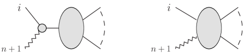
Figure 1: The two types of contributions to a soft limit of an amplitude with $n+1$ particles. The first has a pole when $p_{n+1}\rightarrow 0$ while the second does not. The zig-zag line represents a particle of spin $j$ whose momentum is taken to be soft; straight lines represent particles of spin $j_{i}$ ($i=1,2,...,n$).

At the same time, the gauge invariance of the full amplitude (B.2) with respect to the transformation of the spin $j$ polarization tensor requires that

$$q_{\mu_{j}}{\cal A}^{\mu_{1}\dots\mu_{j}}(p_{1},\dots,p_{n},q)=0\ ,$$ (B.7)

or, equivalently,

$$\sum_{i}\sum_{j^{\prime}_{i}}{p_{i}^{\mu_{1}}\dots p_{i}^{\mu_{j-1}}}\ j^{\prime}_{i}!\ W_{j^{\prime}_{i}}(p_{i}+q,\partial_{u^{\prime}})P_{j^{\prime}_{i}}(p_{i}-q,u^{\prime})+q_{\mu_{j}}N^{\mu_{1}\dots\mu_{j}}(p_{1},\dots,p_{n},q)=0\ .\ \$$ (B.8)

This relation should hold for any $q$, e.g., order by order in a small $q$ expansion. Below we shall focus on the leading order in its small-$q$ expansion.

The leading ${\cal O}(q^{0})$ term obtained by setting $q=0$ in (B.8) gives

$$\sum_{i}\sum_{j^{\prime}_{i}}{p_{i}^{\mu_{1}}\dots p_{i}^{\mu_{j-1}}}\ j^{\prime}_{i}!\ W_{j^{\prime}_{i}}(p_{i},\partial_{u^{\prime}})P_{j^{\prime}_{i}}(p_{i},u^{\prime})=0\ .$$ (B.9)

Here we used the assumption of locality to drop the $N$-term in (B.8) which should not have poles in $q$. Since here $W_{j^{\prime}_{i}}$ (taken at $q=0$) is an on-shell amplitude, it should obey the gauge-invariance constraints (B.6) which imply that only the terms with $j^{\prime}_{i}=0$ are non-vanishing. Then the surviving $W_{0}$ factor becomes simply the same as the scattering amplitude ${\cal A}^{0...0}(p_{1},\dots,p_{n})$ of $n$ spin-$0$ fields, i.e. we get (for any $j$)

$${\cal A}^{0...0}(p_{1},\dots,p_{n})\sum_{i}p_{i}^{\mu_{1}}\dots p_{i}^{\mu_{j-1}}=0\ .$$ (B.10)

As the sum of products of momenta does not, in general, vanish if $j>2$ we conclude that

$${\cal A}^{0...0}(p_{1},\dots,p_{n})=0\ ,$$ (B.11)

i.e. if one starts with a local action then the scalar scattering amplitude should vanish, in agreement with [26].

Note that this conclusion is consistent with the cancellation of the poles of the $0000$ amplitude observed in section 5 where we introduced a local action involving extra fields $\psi_{j}$.

B.2 Expansion of the $j_{1}...j_{n}j$ amplitude

Next, let us generalize the above discussion and consider the consequences of gauge invariance for an amplitude with $n$ particles of generic spins $j_{1},\dots,j_{n}$ (with momenta $p_{1},\dots,p_{n}$) and an additional particle of spin $j$ with soft momentum $p_{n+1}=q$. We will again assume that our starting point is a local interacting Lagrangian. As in the $j_{1}=...=j_{n}=0$ case analysed above, the $q\to 0$ limit of this amplitude then has a singular and a regular contributions shown in fig. 1:

$${\cal A}^{\mu_{1}\dots\mu_{j}}(p_{1},\dots,p_{n},q) \sim \sum_{i}\sum_{j^{\prime}_{i}}V^{\mu_{1}\dots\mu_{j}}_{j,j_{i},j^{\prime}_{i}}(q,p_{i},\partial_{u})\ \frac{P_{j^{\prime}_{i}}(u,u^{\prime})}{2q\cdot p_{i}}\ W_{j^{\prime}_{i}}(p_{i}+q,\partial_{u^{\prime}})$$ (B.13)

$$+\ N^{\mu_{1}\dots\mu_{j}}(p_{1},\dots,p_{n},q)\ .$$

Here we explicitly indicated only Lorentz indices that should be contracted with spin $j$ polarization tensor. As in (B.2), $W_{j^{\prime}_{i}}$ is a Green’s function with all but the $i$-th leg (with momentum $q+p_{i}$) being on shell. For $q\to 0$ it becomes an $n$-point amplitude once it acts on a polarization tensor, and thus it should obey the constraints (B.6).

The covariant three-point vertices $V^{\mu_{1}\dots\mu_{j}}_{j,j_{i},j^{\prime}_{i}}(q,p_{i},\partial_{u})$ can be found in [7]. In the present case (relevant for the discussion of the first diagram in fig. 1) the cubic vertex may be written as

$$V_{j,j_{i},j^{\prime}_{i}}(q,p_{i},p_{i^{\prime}};u_{q};\partial_{u}) \equiv u_{q}^{\mu_{1}}\dots u_{q}^{\mu_{j}}V^{\mu_{1}\dots\mu_{j}}_{j,j_{i},j^{\prime}_{i}}(q,p_{i},p_{i^{\prime}};\partial_{u})$$

$$= c_{jj_{i}j^{\prime}_{i}}\sum_{\stackrel{{\scriptstyle\alpha+\beta+\gamma=n}}{{0\leq n\leq{\rm min}(j,j_{i},j^{\prime}_{i})}}}\frac{1}{\alpha!\beta!\gamma!}((q-p_{i})\cdot\partial_{u})^{j^{\prime}_{i}-n+\gamma}$$

$$(u_{q}\cdot(p_{i}-p_{i^{\prime}}))^{j-n+\alpha}(u_{q}\cdot\partial_{u})^{\beta}\phi_{j_{i}}\big{(}p_{i},(p_{i^{\prime}}-q)^{j_{i}-n+\beta},\partial_{u}^{\alpha},u_{q}^{\gamma}\big{)}\ .$$

Here we assume that the polarization tensor of the external leg $\phi_{i}$ is already a part of $V$ and the argument $u$ corresponds to the internal line with spin $j^{\prime}_{i}$ and momentum $p_{i^{\prime}}$. We also used the notation $\phi_{j}(a^{k},...,b^{n})$ explained in (3.2). The coefficients $c_{jj_{i}j^{\prime}_{i}}$ (fixed in the light-cone gauge approach [4] will be assumed a priori to be arbitrary.

The transformation of $V_{j,j_{i},j^{\prime}_{i}}$ under the spin-$j$ gauge symmetry is given by the contraction of one of its free indices with the momentum $q$, or, alternatively, by replacing one of the vectors $u_{q}$ by $q$. Then the only nontrivial contribution comes from $q\cdot(p_{i}-p_{i^{\prime}})$ term; all other terms cancel out because of the on-shell gauge invariance of the three-point vertex [7], i.e.

$$q\cdot\partial_{u_{q}}V_{j,j_{i},j_{3}}(q,p_{i},p_{i^{\prime}};u_{q};\partial_{u}) = 2q\cdot p_{i}\ c_{jj_{i}j^{\prime}_{i}}\sum_{\stackrel{{\scriptstyle\alpha+\beta+\gamma=n}}{{0\leq n\leq{\rm min}(j,j_{i},j^{\prime}_{i})}}}\frac{1}{\alpha!\beta!\gamma!}((q-p_{i})\cdot\partial_{u})^{j^{\prime}_{i}-n+\gamma}$$ (B.15)

$$\!\!\!\!\!\!\!\!\!\!\!\!\times(u_{q}\cdot(p_{i}-p_{i^{\prime}}))^{\alpha-1}(u_{q}\cdot\partial_{u})^{\beta}\phi_{j_{i}}(p_{i},(p_{i^{\prime}}-q)^{j_{i}-n+\beta},\partial_{u}^{\alpha},u_{q}^{\gamma})$$

$$\equiv 2q\cdot p_{i}\ F_{j,j_{i},j^{\prime}_{i}}(q,p_{i};u_{q};\partial_{u})\ .$$ (B.16)

Therefore, the spin-$j$ gauge invariance of the amplitude (B.13) implies that

$$0 = q\cdot\partial_{u_{q}}(u_{q}^{\mu_{1}}\dots u_{q}^{\mu_{j}}{\cal A}^{\mu_{1}\dots\mu_{j}}(p_{1},\dots,p_{n},q))$$ (B.18)

$$= \sum_{i}\sum_{j^{\prime}_{i}}F_{j,j_{i},j^{\prime}_{i}}(q,p_{i};u_{q};\partial_{u})\ W_{j^{\prime}_{i}}(p_{i}+q,\partial_{u^{\prime}})\ {P_{j^{\prime}_{i}}(u,u^{\prime})}$$

$$+\ q\cdot\partial_{u_{q}}(u_{q}^{\mu_{1}}\dots u_{q}^{\mu_{j}}N^{\mu_{1}\dots\mu_{j}}(p_{1},\dots,p_{n},q))\ .$$

Here the second line is the transformation of the contribution of the first diagram in fig. 1 and the third line represents the transformation of the contribution of the second diagram.

To determine the general consequences of gauge invariance of the amplitude we shall expand (B.18) at small $q$. While there may be interesting information contained in the subleading terms (like, e.g., subleading soft theorems in YM theory [27]), here we shall restrict consideration to the leading $O(q^{0})$ order.

Setting $q=0$ in (B.18) we find (assuming again the locality of the Lagrangian, i.e. the regularity of $N$ in (B.18))

$$0 = \sum_{i}\sum_{j^{\prime}_{i}}F_{j,j_{i},j^{\prime}_{i}}(0,p_{i};u_{q};\partial_{u})\ W_{j^{\prime}_{i}}(p_{i},\partial_{u^{\prime}})\ {P_{j^{\prime}_{i}}(u,u^{\prime})}$$ (B.20)

$$= \sum_{i}\sum_{j^{\prime}_{i}}c_{jj_{i}j^{\prime}_{i}}\sum_{\stackrel{{\scriptstyle\alpha+\beta+\gamma=n}}{{0\leq n\leq{\rm min}(j,j_{i},j^{\prime}_{i})}}}\frac{(-1)^{j^{\prime}_{i}+j_{i}-2n+\gamma+\beta}\ 2^{j+j_{i}-2n+\alpha+\beta-1}}{\alpha!\beta!\gamma!}(p_{i}\cdot\partial_{u})^{j^{\prime}_{i}-n+\gamma}$$

$$\times(u_{q}\cdot p_{i})^{\alpha-1}(u_{q}\cdot\partial_{u})^{\beta}\phi_{j_{i}}(p_{i},p_{i}^{j_{i}-n+\beta},\partial_{u}^{\alpha},u_{q}^{\gamma})\ W_{j^{\prime}_{i}}(p_{i},\partial_{u^{\prime}})\ {P_{j^{\prime}_{i}}(u,u^{\prime})}\ .$$

The transversality of the polarization tensor and the constraints (B.6) imply that all the terms with $j_{i}-n+\beta\neq 0~{}~{}{\rm or}~{}~{}j^{\prime}_{i}-n+\gamma\neq 0$ vanish identically. Therefore, the only nontrivial constraints come from configurations of parameters for which $j_{i}-n+\beta=0$ and $j^{\prime}_{i}-n+\gamma=0$ are satisfied at the same time. Since $\beta,\gamma\geq 0$ and $n\leq{\rm min}(j,j_{i},j^{\prime}_{i})$, the solution to these constraints is

$$j_{i}=j^{\prime}_{i}\leq j~{}~{},\quad n=j_{i}=j^{\prime}_{i}~{}~{},\quad\beta=\gamma=0~{}~{},\quad\alpha=n=j_{i}=j^{\prime}_{i}\ .$$ (B.21)

Then all the sums except the sum over the external particles collapse to a single term and (B.20) reduces to

$$0 = \sum_{i}c_{jj_{i}j_{i}}\frac{1}{j_{i}!}(u_{q}\cdot p_{i})^{j-1}\phi_{j_{i}}(p_{i},\partial_{u}^{j_{i}})\ W_{j^{\prime}_{i}}(p_{i},\partial_{u^{\prime}})\ {P_{j^{\prime}_{i}}(u,u^{\prime})}$$ (B.22)

$$= {\cal A}^{j_{1}...j_{n}}(p_{1},\dots,p_{n})\sum_{i}c_{jj_{i}j_{i}}(u_{q}\cdot p_{i})^{j-1}\ .$$

For $j=2$ we get the constraint that $c_{2j^{\prime}j^{\prime}}$ must be the same for all $j^{\prime}$, i.e. the spin 2 coupling must be universal (then $c_{2j^{\prime}j^{\prime}}$ factorizes and the momentum conservation sets the sum in (B.22) to zero).

For $j>2$ the sum in (B.22) cannot vanish for generic on-shell momenta; it follows then that the gauge invariance requires that either all the $j_{1}...j_{n}$ amplitudes should vanish

$${\cal A}^{j_{1}...j_{n}}=0\ ,$$ (B.23)

or we should have the following constraint on the three-point coupling constants

$$c_{jj_{i}j_{i}}=0~{},\ \ \ \ \ \ \ \ ~{}~{}j_{i}<j\ .$$ (B.24)

The latter condition (found earlier in [11]) (B.24) means that there should be no cubic diagonal coupling (B.2) of a spin-$j$ field with all smaller $j_{i}<j$ spins. In our discussion of the $0...0j$ amplitude in the previous subsection we assumed that $c_{j00}\not=0$ and thus arrived at (B.23), i.e. (B.11).

The 3-point coupling constants found in the light-cone approach in [4] do not satisfy (B.24) and then one should either relax the assumption of locality of the interaction Lagrangian or accept the vanishing of the scattering amplitudes (B.23).

Appendix C Vanishing of the trace contribution to four-graviton amplitude

Below we sketch the argument for the vanishing of the on-shell matrix element of the graviton trace contribution in the $\partial_{m}t_{mn}=0$ gauge, i.e. of $Y_{4}$ in (6.1), for a special choice of on-shell gauge, i.e. for a special choice of the polarization tensors.

Let us for definiteness consider the amplitude where the particles $1$ and $2$ have negative helicity (-2) while the particles $3$ and $4$ have positive helicity (+2). The main point is that using the on-shell gauge invariance it is possible to choose the 4 polarization tensors $\varepsilon^{\pm}(p)$ in such a way that the following combinations with some free indices are simultaneously zero

$$\varepsilon^{-}(p_{1})_{ac}\,\varepsilon^{-}(p_{2})_{bc}\,\varepsilon^{+}(p_{3})_{kn}\,\varepsilon^{+}(p_{4})_{mn}=0\ ,\qquad\varepsilon^{-}(p_{1})_{ac}\,\varepsilon^{+}(p_{3})_{kc}\,\varepsilon^{-}(p_{2})_{bn}\,\varepsilon^{+}(p_{4})_{mn}=0\ ,$$

$$\varepsilon^{-}(p_{1})_{ac}\,\varepsilon^{+}(p_{4})_{mc}\,\varepsilon^{-}(p_{2})_{bn}\,\varepsilon^{+}(p_{3})_{kn}=0\ .$$ (C.1)

Since the matrix element of $Y_{4}$ in (6.1) is given by a linear combination of such products it then vanishes.

The reason for the relations (C.1) is the following. In the spinor helicity notation the graviton polarization tensor may be represented as (for each helicity choice) $\varepsilon^{\pm}(p)=\varepsilon^{\pm}(p)\otimes\varepsilon^{\pm}(p)$ where $\varepsilon$ is the polarization vector, i.e. $\varepsilon^{-}(p)=|q]\langle p|/[qp]$,     $\varepsilon^{+}(p)=|q\rangle[p|/\langle qp\rangle$. Here $q=|q\rangle[q|$ is an arbitrary null vector, which can be chosen independently for each polarization vector; this reflects the remaining on-shell gauge invariance. Once chosen, these reference vectors are not changed from graph to graph. The gauge transformation $\varepsilon^{\mu}\rightarrow p^{\mu}$ translates into $|q\rangle\mapsto|p\rangle$ and $|q]\mapsto|p]$.

Choosing $q_{1}=q_{2}$ and $q_{3}=q_{4}$, the scalar products of the polarization vectors become

$$\varepsilon^{-}(p_{1})\cdot\varepsilon^{-}(p_{2})\sim[q_{1}q_{2}]=[q_{1}q_{1}]=0\ ,$$

$$\varepsilon^{-}(p_{1})\cdot\varepsilon^{+}(p_{3})\ \varepsilon^{-}(p_{2})\cdot\varepsilon^{+}(p_{4})\sim[q_{1}p_{3}][q_{1}p_{4}]\langle q_{3}p_{1}\rangle\langle q_{3}p_{2}\rangle\ ,$$

$$\varepsilon^{-}(p_{1})\cdot\varepsilon^{+}(p_{4})\ \varepsilon^{-}(p_{2})\cdot\varepsilon^{+}(p_{3})\sim[q_{1}p_{4}][q_{1}p_{3}]\langle q_{3}p_{1}\rangle\langle q_{3}p_{2}\rangle\ .$$ (C.2)

Then choosing, e.g., $q_{1}=q_{2}=p_{3}$ and $q_{3}=q_{4}=p_{1}$ sets to zero the last two products in (C.2) and thus implies (C.1) and, as a consequence, the vanishing of the matrix element of $Y_{4}$.

The above choice simplifies also the on-shell matrix elements of $\bar{X}_{3}$ in (6.14) and $\bar{X}_{4}$ in (6.15) since whenever two external on shell polarization tensors are contracted over (at least) one index they do not contribute to the amplitude. For example, in $\bar{X}_{4}$ there are always at least two $t_{mn}$ tensors contracted over one index, so with the above choice of the polarization tensors the contribution of this local four-point vertex to the amplitude also vanishes. This mirrors what happens in gauge theory where a similar choice of the reference vectors $q_{i}$ sets to zero the contribution of the four-point contact term in the YM action to the tree-level four-gluon amplitude; then the full amplitude is given just by the exchange contribution.

References

- [1] X. Bekaert, N. Boulanger, and P. Sundell, “How higher-spin gravity surpasses the spin two barrier: no-go theorems versus yes-go examples,” Rev. Mod. Phys. 84 (2012) 987–1009, [arXiv:1007.0435]. M. Porrati, “Old and New No Go Theorems on Interacting Massless Particles in Flat Space,” arXiv:1209.4876.
- [2] A. K. H. Bengtsson, I. Bengtsson, and L. Brink, “Cubic Interaction Terms for Arbitrary Spin,” Nucl. Phys. B227 (1983) 31. A. K. H. Bengtsson, I. Bengtsson, and N. Linden, “Interacting Higher Spin Gauge Fields on the Light Front,” Class. Quant. Grav. 4 (1987) 1333.
- [3] F. A. Berends, G. J. H. Burgers, and H. Van Dam, “On Spin Three Selfinteractions,” Z. Phys. C24 (1984) 247; “On the Theoretical Problems in Constructing Interactions Involving Higher Spin Massless Particles,” Nucl. Phys. B260 (1985) 295.
- [4] R. R. Metsaev, “Poincare invariant dynamics of massless higher spins: Fourth order analysis on mass shell,” Mod. Phys. Lett. A6 (1991) 359. “S matrix approach to massless higher spins theory. 2: The Case of internal symmetry,” Mod. Phys. Lett. A6 (1991) 2411. “Generating function for cubic interaction vertices of higher spin fields in any dimension,” Mod. Phys. Lett. A8 (1993) 2413. “Cubic interaction vertices of massive and massless higher spin fields,” Nucl. Phys. B759 (2006) 147–201 [hep-th/0512342]
- [5] A. Fotopoulos and M. Tsulaia, “Gauge Invariant Lagrangians for Free and Interacting Higher Spin Fields. A Review of the BRST formulation,” Int. J. Mod. Phys. A24 (2009) 1 [arXiv:0805.1346]. “On the Tensionless Limit of String theory, Off - Shell Higher Spin Interaction Vertices and BCFW Recursion Relations,” JHEP 11 (2010) 086. [arXiv:1009.0727].
- [6] N. Boulanger, S. Leclercq, and P. Sundell, “On The Uniqueness of Minimal Coupling in Higher-Spin Gauge Theory,” JHEP 08 (2008) 056. [arXiv:0805.2764].
- [7] R. Manvelyan, K. Mkrtchyan, and W. Ruhl, “General trilinear interaction for arbitrary even higher spin gauge fields,” Nucl. Phys. B836 (2010) 204 [arXiv:1003.2877] “A Generating function for the cubic interactions of higher spin fields,” Phys. Lett. B696 (2011) 410 [arXiv:1009.1054]
- [8] A. Sagnotti and M. Taronna, “String Lessons for Higher-Spin Interactions,” Nucl. Phys. B842 (2011) 299 [arXiv:1006.5242].
- [9] R. R. Metsaev, “BRST-BV approach to cubic interaction vertices for massive and massless higher-spin fields,” Phys. Lett. B 720, 237 (2013) [arXiv:1205.3131].
- [10] X. Bekaert, N. Boulanger and S. Leclercq, “Strong obstruction of the Berends-Burgers-van Dam spin-3 vertex,” J. Phys. A 43, 185401 (2010) [arXiv:1002.0289].
- [11] M. Taronna, “Higher-Spin Interactions: four-point functions and beyond,” JHEP 1204, 029 (2012) [arXiv:1107.5843].
- [12] P. Dempster and M. Tsulaia, “On the Structure of Quartic Vertices for Massless Higher Spin Fields on Minkowski Background,” Nucl. Phys. B 865, 353 (2012) [arXiv:1203.5597].
- [13] D. Ponomarev and A. A. Tseytlin, “On quantum corrections in higher-spin theory in flat space,” JHEP 1605, 184 (2016) [arXiv:1603.06273].
- [14] A.A. Tseytlin, “On higher spin scattering in flat space”, talk at the workshop “Aspects of Higher-spin theories”, MIAPP, Munich, 23-25 May 2016.
- [15] A. K. H. Bengtsson, “Investigations into Light-front Interactions for Massless Fields (I): Non-constructibility of Higher Spin Quartic Amplitudes,” JHEP 1612, 134 (2016) [arXiv:1607.06659]. “Quartic amplitudes for Minkowski higher spin,” arXiv:1605.02608.
- [16] C. Sleight and M. Taronna, “Higher-Spin Algebras, Holography and Flat Space,” arXiv:1609.00991.
- [17] D. Ponomarev and E. D. Skvortsov, “Light-Front Higher-Spin Theories in Flat Space,” arXiv:1609.04655. D. Ponomarev, “Off-Shell Spinor-Helicity Amplitudes from Light-Cone Deformation Procedure,” JHEP 1612, 117 (2016) [arXiv:1611.00361].
- [18] M. Taronna, “On the Non-Local Obstruction to Interacting Higher Spins in Flat Space,” arXiv:1701.05772 [hep-th].
- [19] M. A. Vasiliev, “Algebraic aspects of the higher spin problem,” Phys. Lett. B 257, 111 (1991). “Higher spin gauge theories: Star product and AdS space,” In *Shifman, M.A. (ed.): The many faces of the superworld* 533-610 [hep-th/9910096].
- [20] E. S. Fradkin and G. A. Vilkovisky, “Conformal Off Mass Shell Extension and Elimination of Conformal Anomalies in Quantum Gravity,” Phys. Lett. 73B, 209 (1978).
- [21] E. S. Fradkin and A. A. Tseytlin, “Conformal Supergravity,” Phys. Rept. 119, 233 (1985).
- [22] A. Y. Segal, “Conformal higher spin theory,” Nucl. Phys. B 664, 59 (2003) [hep-th/0207212].
- [23] E. Joung, S. Nakach and A. A. Tseytlin, “Scalar scattering via conformal higher spin exchange,” JHEP 1602, 125 (2016) [arXiv:1512.08896].
- [24] M. Beccaria, S. Nakach and A. A. Tseytlin, “On triviality of S-matrix in conformal higher spin theory,” JHEP 1609, 034 (2016) [arXiv:1607.06379].
- [25] F. E. Low, “Bremsstrahlung of very low-energy quanta in elementary particle collisions,” Phys. Rev. 110, 974 (1958).
- [26] S. Weinberg, “Photons and Gravitons in s Matrix Theory: Derivation of Charge Conservation and Equality of Gravitational and Inertial Mass,” Phys. Rev. 135, B1049 (1964). “Infrared photons and gravitons,” Phys. Rev. 140, B516 (1965).
- [27] Z. Bern, S. Davies, P. Di Vecchia and J. Nohle, “Low-Energy Behavior of Gluons and Gravitons from Gauge Invariance,” Phys. Rev. D 90, no. 8, 084035 (2014) [arXiv:1406.6987].
- [28] C. Fronsdal, “Massless Fields with Integer Spin,” Phys. Rev. D18 (1978) 3624.
- [29] X. Bekaert, E. Joung and J. Mourad, “On higher spin interactions with matter,” JHEP 0905, 126 (2009) [arXiv:0903.3338].
- [30] C. Sleight and M. Taronna, “Higher Spin Interactions from Conformal Field Theory: The Complete Cubic Couplings,” Phys. Rev. Lett. 116, no. 18, 181602 (2016) [arXiv:1603.00022].
- [31] B. S. DeWitt, “Quantum Theory of Gravity. 3. Applications of the Covariant Theory,” Phys. Rev. 162, 1239 (1967).
- [32] F. A. Berends and R. Gastmans, “On the High-Energy Behavior in Quantum Gravity,” Nucl. Phys. B 88, 99 (1975).
- [33] M. H. Goroff and A. Sagnotti, “The Ultraviolet Behavior of Einstein Gravity,” Nucl. Phys. B 266, 709 (1986).
- [34] S. Sannan, “Gravity as the Limit of the Type II Superstring Theory,” Phys. Rev. D 34, 1749 (1986).
- [35] J. Erdmenger, “Conformally covariant differential operators: Properties and applications,” Class. Quant. Grav. 14, 2061 (1997) [hep-th/9704108].
- [36] S. Deser, M. T. Grisaru, P. van Nieuwenhuizen and C. C. Wu, “Scale Dependence and the Renormalization Problem of Quantum Gravity,” Phys. Lett. B 58, 355 (1975).
- [37] F. Englert, C. Truffin and R. Gastmans, “Conformal Invariance in Quantum Gravity,” Nucl. Phys. B 117, 407 (1976).
- [38] N. C. Tsamis and R. P. Woodard, “No New Physics in Conformal Scalar - Metric Theory,” Annals Phys. 168, 457 (1986).
- [39] S. Ferrara, R. Kallosh and A. Van Proeyen, “Conjecture on hidden superconformal symmetry of Supergravity,” Phys. Rev. D 87, no. 2, 025004 (2013) [arXiv:1209.0418].
- [40] R. Britto, F. Cachazo, B. Feng and E. Witten, “Direct proof of tree-level recursion relation in Yang-Mills theory,” Phys. Rev. Lett. 94, 181602 (2005) [hep-th/0501052].
- [41] R. Gastmans, R. Kallosh and C. Truffin, “Quantum Gravity Near Two-Dimensions,” Nucl. Phys. B 133, 417 (1978).
- [42] G. ’t Hooft and M. J. G. Veltman, “One loop divergencies in the theory of gravitation,” Ann. Inst. H. Poincare Phys. Theor. A 20, 69 (1974).
- [43] E. D. Skvortsov and M. A. Vasiliev, “Transverse Invariant Higher Spin Fields,” Phys. Lett. B 664, 301 (2008) [hep-th/0701278].
- [44] D. Francia and A. Sagnotti, “Free geometric equations for higher spins,” Phys. Lett. B 543, 303 (2002) [hep-th/0207002].