Origin of spatial organization of DNA-polymer in bacterial chromosomes.

Abstract

In-vivo DNA organization at large length scales ($\sim 100nm$) is highly debated and polymer modelshave proved useful to understand the principle of DNA-organization. Here, we show that $<2$% cross-links at specific points in a ring polymer can lead to a distinct spatial organization of the polymer. The specific pairs of cross-linked monomers were extracted from contact maps of bacterial DNA.We are able to predict the structure of 2 DNAs using Monte Carlo simulations of the bead-spring polymer with cross-links at these special positions. Simulations with cross-links at random positions along the chain show that the organization of the polymer is different in nature from the previous case.

It is established that DNA-polymer is not a random coil in either bacterial cells Le et al. (2013); Joyeux (2015); Cagliero et al. (2013) or in eukaryotic cells Lieberman-Aiden et al. (2009); Bickmore and van Steensel (2013); Sexton et al. (2012); Tjong et al. (2012). Experimental methods such as CCC (chromosomal conformation capture) which was then further developed as 5C and then Hi-C have consistently shown the presence of topologically associated domains (TADs) in the contact maps (C-maps) of DNA-chains Dixon et al. (2012); Jonathan D. Halverson and Grosberg (2014); Dekker et al. (2013). The Hi-C technique gives us the C-map which is the map of frequencies that a segment of the DNA chain (say $i$) is found in spatial proximity to another segment (say $j$) for all combinations $i,j$ of segments along the contour length of the DNA-polymer. TADs are patches in C-maps which indicate that some segments of the chain (at 1 mega-base pair(BP) to 1 kilo-BP resolution), are found spatially close to other particular segments with higher frequencies compared to the rest of the segments.

The ds-DNA is stiff at length scales of $1$nm but can be considered to be a flexible chain at length scales beyond $100$nm Rob Phillips (2008) . The persistence length $\ell_{p}$ of a naked DNA is 150 Base Pairs (BP) $\equiv 50$ nm Rubinstein and Colby (2003) and the value of $\ell_{p}$ in vivo is debated Maeshima et al. (2010). Since, the resolution of Hi-C experiments are well above this length scale Lieberman-Aiden et al. (2009); Le et al. (2013), there has a focussed attempts in the last few years trying to understand the DNA organization and in particular origin of formation of TADs from the principles of polymer physics Pombo and Nicodemi (2014); Gilbert et al. (2017); Fudenberg et al. (2016a); Mirny (2011); Rosa and Everaers (2008). A series of studies indicate that TADs in eukaryotic cells are indicative of fractal globule organization of the polymer (as opposed to equilibrium globule) Lieberman-Aiden et al. (2009); Imakaev et al. (2015). Recently, more detailed polymer models with either different lengths of loops or with many distinct (coarse-grained) diffusing binder molecules which cross-link different segments of the chain have reproduced TADs of sections of a particular eukaryotic DNA by performing optimizations in multi-parameter space. Distinct kinds of binder molecules link correspondingly distinct monomers (DNA-segments) along the chain, and the optimization parameters include the number of distinct kind of binders/monomers as well as the position and number of distinct monomers as well as diffusing cross-links along the contour Barbieri et al. (2012); Fudenberg et al. (2016b, a); Goloborodko et al. (2016).

We propose a much simpler model for shorter bacterial DNAs and ask a more general question: Does fixed cross-links (CLs) at a few specific positions along the polymer chain contour organize the polymer into a particular architecture? If so, can we predict the global shape/structure of the DNA polymer and does it reproduce the C-map or at least parts of it? The position of the cross-links are chosen by using the C-map to identify the highest frequencies of two segments to be in spatial proximity. We cross-link a minimal number of these segments, and then computationally cross-check if the other segments of the polymer get localized in space and with respect to each other. Of course the chain can fluctuate due to thermal fluctuations but maintaining the architecture. We then compare this polymer organization with the organization obtained when a ring-polymer (most bacterial DNAs are ring polymers) has an equal number of CLs at randomly chosen positions along the chain contour. We choose $10$ different realizations of randomly positioned CLs. On comparing we see that nature chooses the position of CLs carefully such that the architecture of the DNA-polymer is well organized in a manner very distinct from what is obtained for a polymer with random CLs.

We investigate the organization of two bacterial DNAs, E. Coli and C. Crescentus. Each has a single chromosome of length $4$ Mega-BP: we choose to work with shorter bacterial DNA with just one chromosome and no nucleus wall. DNA is modeled as a flexible bead spring ring polymer (both bacterial chromosomes are ring polymers) with a harmonic spring potential $\kappa(r-a)^{2}$ acting between neighbouring beads; the choice of $a=1$ ($\sim 100$ nm) sets the length scale of the problem. The excluded volume(EV) of the beads are modelled by suitably truncated purely repulsive Lennard-Jones potential with $\sigma=0.2a$. The E.coli and C.Crescentus DNAs have $4642$ and $4017$ kilo-BPs, which we model by $4642$ and $4017$ monomers, respectively. The naked DNA Kuhn segment has just 300 BPs Rubinstein and Colby (2003) whereas a bead represents 1000 BPs. The effects of DNA coiling around histone-like proteins occurs at smaller length scales; longer range effects due supercoiling, presence of plectonemes etc. should show up in the C-map and their effects gets incorporated as cross-links at the length scales we consider. Moreover, bacterial DNA occupy $15-25$% of cellular volume, so we choose to ignore confinement effects, if any. Instead, we fully focus on the role of CLs in the organization of the polymer. The introduction of CLs between segments of the chain in our model can be justified due the presence of DNA-binding proteins which are present in bacterial cells (as well as higher eukaryotic cells) Joyeux (2015); Dixon et al. (2012); Phillips and Corces (2009); Ohlsson et al. (2010).

We model the cross-links between two segments of the DNA-polymer by a harmonic potential [$\kappa(r-a)^{2}$, where $\kappa=200k_{B}T/a^{2}$] between two monomer beads. The two “cross-linked” monomers (CLs) are typically well separated along contour of the model polymer. We cross-link pair of monomers if they are found spatially close above a certain frequency in C-maps. By lowering the frequency cutoff, we can have more cross-linked monomers. For details, refer Agarwal et al. (2017). So, we take $47$ or $159$ CLs for E. Coli. For C.Crescentus we take $49$ or $153$ CLs which we refer as BC-1 and BC-2, respectively. The list of cross-linked monomers are listed in Table SLABEL:tab:table1. From the table one observes that a pair of neighbouring monomers along the chain contour can get cross-linked to another pair of neighbouring monomers, hence the number of actual CLs are fewer (refer Table LABEL:tab:table1 for examples and detailed explanations) . Removing such over-counts, there are $26$ and $60$ effective CLs for C.Crescentus. For E. Coli we have $27$ and $82$ effective CLs, CL-list and other details are in Agarwal et al. (2017). We also investigate large scale organization of the chain when we have a set of CLs, where pairs of monomers are chosen randomly and cross-linked. A set of $26$ and $60$ CLs at random positions in a ring of $4017$ monomers is referred as RC-1 and RC-2, respectively.

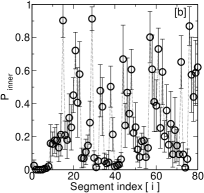
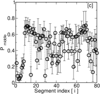
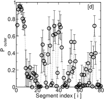
Figure 1: (a) shows that the $R_{g}$ of C.Crescentus DNA for 9 runs, each starting from independent initial conditions for BC-1 and BC-2 sets of CLs. It also shows $R_{g}$ data for random set of CLs: RC-1 and RC-2 for 10 different choices of random cross-links sets, set-index is on x-axis. The error bar shown for $R_{g}$ is the standard deviation (SD) calculated from $9$ indepedent runs for a particular set of CLs. Subplots (b),(c) and (d) show the probability $P_{inner},\,P_{middle},\,P_{outer}$ of finding a segment $i$ in the inner, middle and outer regions, respectively, of the DNA-coil for BC-2. The error bar is the SD calculated from $9$ independent runs.

I Results

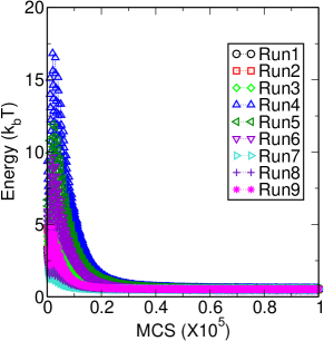
Figure S3: Plot shows the potential energy of the polymer chain with CLs as it relaxes to the same value of the potential energy.Each of the $9$ runs start with independent initial configuration of the polymer.

To establish that sets of bio-CLs lead to a particular organization of the polymer, we start from $9$ different initial configurations of a ring polymer, and allow the chain to equilibrate using Monte Carlo (MC) simulations using Metropolis algorithm. After equilibration (inherently non-equilibrium biological systems at a certain stage of their cell cycle can be thought of to be in a state of local equilibrium), we compare statistical quantities which provide us evidences about structure and conformations of polymer chains. If we get similar structure from all $9$ runs, we could claim that CLs lead to particular sets of conformation at large length-scales. We take care to choose the $9$ different initial configurations of polymers in ways that we ensure that the cross-linked monomers are at very different relative positions with respect to each other, moreover, distance between them can be much larger than their equilibrium distance $a$. Thus the initial potential energy of the system will be high (Fig.S3), and as the system relaxes due to the presence of CLs through MC moves, the average energy of the polymers in each run should have nearly the same value at the end of equilibration run. After equilibration, the polymer explores phase space over $12$ million iterations in each run to calculate statistical quantities with thermal energy scale $k_{B}T=1$. Small EV of the beads allows chains to cross each other, moreover we take a large MC displacement of $1.2\sigma$ in every 100 steps. These help in releasing any artificial topological constraints induced by intial configuration. Chain crossing is justified due to the activity of topoisomerase II.

We repeat these calculations using RC-1 and RC-2 CLs and compare polymer organization with those obtained using BC-1 & BC-2. To firmly establish that the BC-1 and BC-2 set of CLs lead to an organization of the ring polymer which is very distinct from the organization achieved with random CLs, we choose $10$ independent sets of random CLs, then for each set of CLs gave $9$ runs starting from $9$ independent initial positions. After equilibration, we compare the differences in the large-scale organization. For each random CL-set, RC-1 CLs are a subset of RC-2 CL set. We show later that the reason for the distinct organizaton of the chain with BC-2 is in turn the very distinct spatial organization of the CLs themselves in space, which in turn comes from choice of monomers which are cross-linked.

The primary problem is how to identify large scale organization of a single floppy polymer chain and come up with a prediction of relative position of different segments, when rapid comformation changes are inherent in the system. Quantities like pair correlation function $g(r)$ between monomers are insufficient as we would like more individualized information about arrangement of different segments of the DNA. We use the following four quantities to identify the global organization of C.Crecentus DNA-polymers; similar detailed data for E.coli is given in Agarwal et al. (2017)

1. We estimate the radius of gyration $R_{g}$ of the DNA-polymer of C.Crescentus. The value of $R_{g}$ obtained is $\approx 8a$ from all the $9$ runs for BC-1, and $\approx 6.5a$ for BC-2. Data is shown in Fig 1a. In contrast, $R_{g}$ decreases from $8a$ to $6a$, when number of CLs are increased from RC-1 to RC-2 for each set of random CLs. The decrease is more significant for random CLs, as would be expected for a polymer chain with more constraints. A smaller relative decrease in $R_{g}$ as we change from BC-1 to BC-2 compared to the change from RC-1 $\rightarrow$ RC-2 is the first indication of distinct organization of the coil with bio-CLs. A ring polymer with $4017$ monomers without any CLs has $R_{g}$ value of $11$.

2. We divide the polymer into segments of $50$ monomers each, and identify whether the center of mass (CM) of each segment is to be found in the inner, middle or outer section of the coil. Thereby the polymer has $80$ segments. We define a segment to be in inner/middle/outer section if the distance $r$ of segment’s CM from the CM of the coil is ($r<5a$), /($5a<r<9a$), /($r>9a$), respectively. If a segment $i$ is found to be in the same section in all the $9$ independent runs, we can claim that all $9$ chains are similarly organized. Data in Fig.1 b,c,d, confirms and validates the above claim. As we see in Fig.1b, the same segments are found inside of the coil with higher probability, some are more likely to be found in the middle region, and the rest in the outer region. However, the values of probabilities $P_{inner},P_{middle},P_{outer}$ for a segment statistically fluctuate across runs.

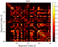
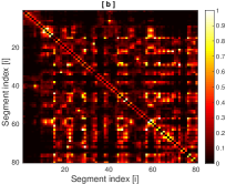
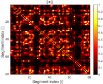
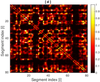
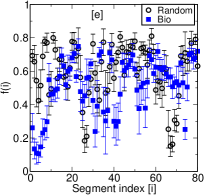
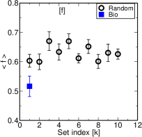
Figure 2: The colormaps give the probability of finding the CM of segment $i$ and $j$ within a distance cutoff of $R^{C}=5a$ for a DNA polymer with cross-links. Figure (a),(b) correspond to two independent runs starting with different initial configurations for BC-2. and (c),(d) correspond to the runs with different intial conditions for RC-2. Data for additional runs for BC-1, BC-2 and RC-1, RC-2 are given in Fig.S1. In plot (e) the x-axis shows segment index and y-axis shows [$f(i)$] which is the number of pixels with probability $p(i,j)>0.05$ (non-dark pixels) divided by the total number of segments in subplots (a),(b),(c),(d) for BC-2 and RC-2 respectively. Error bars shows the fluctuations in the value of $f(i)$ across independent $9$ initial conditions. Subplot (f) shows the average value of $f(i)$ ($\langle f\rangle$)for $10$ random CL-sets and $1$ bio-CL set BC-2.

3. Instead of calculating $g(r)$, we aim to identify which segments (say $i$) are near other segments (say $j$) with higher probability. We can calculate this probability for each pair of segments and show this in a color-map, where both the axes represent segment indices and the color of each pixel denotes the probability that the CM of segments $i$ and $j$ are within distance of $R^{C}<5a$. We show data from two runs for BC-2 in Fig.2 (a,b). For comparison we also show data RC-2 in Fig.2 (c,d) , respectively. Colormaps of bio-CLs and random-CLs in Fig.2 show that there is higher probability (color red) of finding only certain segments near others, and some segments are never found in proximity of certain other segments (color black). This indicates a certain degree of organization of segments. Large fluctuations in the conformation of polymer would result in a colormap which would be predominantly dark, indicating that there is almost equal (and small) probability of different segments to be near each other(Fig.S1). Moreover, colormaps from independent runs and same CL set show statistically similar patterns of red and dark pixels: this implies the same organization of segments in independent runs.

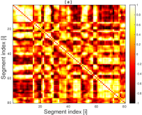
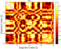
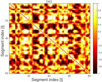
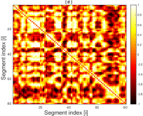
Figure 3: The set of 4 colormaps give the probability of finding the angular correlations between segment $i$ and segment $j$ of a ring polymer. Figure (a),(b) correspond to independent runs of the C.Crescentus DNA-polymers with BC-2 set of CLs. Subplots (c),(d) are for runs with CL-set RC-2. Colormaps from additional runs for BC-1, BC-2, RC-1 and RC-2 are given in Fig.S2.

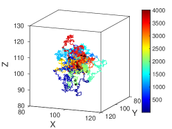
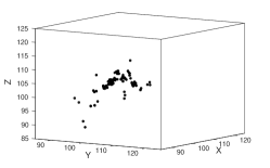
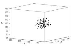
Figure S6: Representative snaphots of the polymer with BC-2(top) CLs form our simulation. Black circles show the positions of the CLs. The monomers are colored from blue to red along the chain contour. The positions of CLs for BC-2, RC-2 is also shown in middle, bottom figures where the polymer is not shown for better visualization. From the plots we see that CLs are clustered in space for BC-2 and are scattered for RC-2.

For BC-1/RC-1, we cannot identify large scale structural organization of the polymer, nor can one distinguish between the colormaps of BC-1 and RC-1. In contrast, on comparing colormaps of BC-2 and RC-2 (Fig.2) we can infer that the character of organization of the polymer is different in the two cases. We find large red patches separated by dark rows/columns in the colormaps for BC-2, whereas, for RC-2 colormaps the lighter pixels are relatively more scattered. This is further quantified in Fig.2e, where we see that a chain segment is approached by fewer other segments for BC-2 as compared to RC-2. For each of the random CL-sets, each segment can be near a larger number of segments as can be deduced from the higher value of $\langle f\rangle$ in Fig.2f. This observation, coupled with the fact that polymer has higher value of $R_{g}$ and more segments in the outer region for BC-2 when compared with data for RC-2(Fig.S6), implies that certain segments have well defined neighbouring segments (more structure) as compared to polymer with RC-2. The neighbouring segments could be far away along the contour length but are neighbours spatially. Thus, the positions of bio-CLs along the contour are special (not random) for BC-2, as these result in distinctive meso-scale organization of the DNA.

We emphasize that the colormaps of Fig.2 look similar to the C-maps of DNA-polymer which we use as modelling input. But the content is very different in the sense we obtain large scale structural correlations of the entire polymer chain from our colormaps. To reiterate, C-maps give us input about the location of CLs along the polymer contour at the length scale of monomers, our color-maps show how various segments (each of 50 monomers) are organized relative to each other in space.

4. We next focus on relative angular position of polymer segments with respect to the CM of the DNA globule. For each pair of segments $i,j$ we calculate if the vectors $\vec{r_{i}}$ and $\vec{r_{j}}$, joining the CM of globule to the CM of the segments $i,j$, subtend an angle of more than $\pi/2$ radians. If the angle $\theta$ between $\vec{r_{i}}$ and $\vec{r_{j}}$ is $>\pi/2$, then we interpret that the two segments lie in opposite hemispheres, else the two segments lie on the same side of the globule w.r.t the CM of the polymer. We compute the average of the counter $\delta^{ij}_{\theta}$ for each pair of segments $i,j$ as follows: for a microstate $\delta^{ij}_{\theta}$ is incremented by $1$ if $\cos(\theta)<0$, and decremented by $1$ if $\cos(\theta)<0$. We plot the value of $\langle\delta^{ij}_{\theta}\rangle$ $N^{ave}$ in Fig.3 for each pair of $i-j$ for BC-1,BC-2,RC-1,RC-2 CLs. The value of $\langle\delta^{ij}_{\theta}\rangle$ varies from $-1$ to $1$.

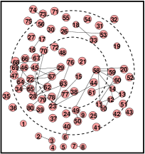
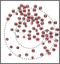
Figure 4: The 2-d maps of DNA organization of C. Crescentus and E.coli bacteria above the $100$ nm length scale using BC-2. This is obtained using the statistical data presented in this manuscript, and in Agarwal et al. (2017) for E.Coli. The links between different circles indicate that colormaps show these segments to be spatially close to each other though they look separated on the map.

The interpretation of data presented in Fig.3 is similar to that of Fig.2. If the pixel corresponding to segments $i,j$ is bright, then they are angularly close w.r.t. coil CM, and a dark pixel indicates they lie predominantly on opposite hemispheres. An orange pixel corresponds to the value of $\langle\delta^{ij}_{\theta}\rangle\approx 0$. If $\langle\delta^{ij}_{\theta}\rangle\approx 0$ then we cannot interpret their relative angular locations. An orange pixel does not imply $\theta\approx\pi/2$ because one can also get $\langle\delta^{ij}_{\theta}\rangle\approx 0$ if the segments lie close to center of the coil and can rapidly change their relative positions by small spatial displacements. This would lead to $\langle\delta^{ij}_{\theta}\rangle\approx 0$. For BC-1 and RC-1 CL sets(Fig.S2), we again see that the patterns of bright and dark pixels are almost identical from independent runs. In contrast, the colormaps for BC-2 in Fig.3 (a,b) and RC-2 in (c,d) are immediately distinguishable. The BC-2 data show large patches of bright pixels indicating that adjacent segments along the contour are on the same side of the globule. The dark and bright pixels for RC-2 is relatively more distributed/scattered. Furthermore, more detailed discussion on the reasons for differences color-maps in Fig.2 and 3 for BC-2 are given in Supplementary section.

Finally, using the aggregate of all the structural quantities presented in Figs.1,2, 3 we are able to piece together the large scale organization of DNA-polymers in a 2D map for both C.Crescentus and E. Coli(Fig.4). For details see supplementary section: Construction of 2-D map. Corresponding structural quantities/colormaps for E. Coli can be found in Agarwal et al. (2017); the interpretation and conclusions are similar to what is discussed above for C.Crescentus.

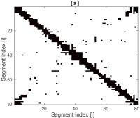
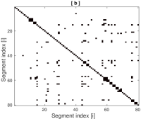
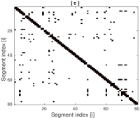
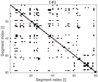
Figure 5: Plots (a), (b) show binary version of the coarse-grained experimental C-map and color map obtained from simulations respectively, for C. Crecentus. Plots (c),(d) are corresponding data for E.Coli. To be able to compare easily by the eye, we have color coded all the frequencies $f$ [probabilities $p$] with value $f>0.0001$ [$p>0.5$] as black for experimental [simulation] colormaps. The corresponding actual (non-binary) coarse-grained experimental data is given in Fig.S4

In lieu of the future experiments which can confirm our predictions, we can use the information content of the contact map to validate our prediction of DNA-organization. To be able to compare the positional colormaps obtained from our simulations to the experimental C-map, we condense the data of C-maps into a $80\times 80$ matrix by suitable coarse-graining (averaging over neighbouring bins) of the frequency data of C-maps. We can now compare the coarse-grained experimental C-map (which now give proximity frequencies of large sections of the DNA) with the highest probabilities ($>0.5$) of the color-maps (generated by our simulations) as shown in Fig. 5, these show a good match with each other. This is by no means an obvious match: we take very few (but significant) points from the C-map as cross-linked monomers in our simulations, and are able to predict from our simulations the positions of highest contact frequencies in the coarse-grained C-map. In addition, we generate from our simulations the radial position of segements, angular positions of segments which is not available in the C-maps. The difference between the coarse-grained experimental and simulation color-map for C.Crecentus is the absence of clear high-probability diagonals in our colormap. The plausible reason for the presence of the diagonal and off-diagonal bright patches in the experimental C-map could be the presence of plectonemes as proposed in Le et al. (2013). The effect of plectonemes are not accounted for in our model as we have taken only 153 CLs which translate to only 60 effective CLs. But using these CLs our simulation C-maps matches accurately with the high probablity pixels for segments far separated along the contour in the experimental C-map. Furthermore, the cutoff distance $R^{C}=5a$ we choose while generating colormaps is comparable to the $R_{g}\approx 4a$ of 50 segments. Thereby, only few segment CMs can occupy positions within distance $R^{C}$.

To summarize, we show that the underlying mechanism of meso-scale organization in E. Coli and C.Crescentus DNA involves constraints (cross-links) at specific positions along the chain contour. Also we predict the overall 2D architecture of the bacterial genomes. We observe that the nature of the organization is different for polymers with the CLs taken from the experimental C-maps and for polymers with CL-positions chosen randomly. Our preliminary understanding for this difference is that for bio-CLs multiple CLs get clumped together spatially (Fig.S??). As a consequence multiple segments of the chain are pulled in together towards the center of the coil with loops remaining on the outside. This can be reconfirmed also for E.Coli in Agarwal et al. (2017). In contrast for RC-2 set of CLs the CLs are scattered in space. We have also shown that a minimal number (around $\sim 3\%$ of monomers) of CLs are required for a polymer to get organized in a particular structure as we do not get any organization in the case of BC-1 and RC-1. We have checked lack of clear polymer organization with the number of CLs in between BC-1 and BC-2.

Supplementary Materials

II List of cross-linked monomers in our simulations.

In the following table, we list the monomers which are cross-linked to model the constraints for the DNA of bacteria C. Crecentus. Note that for random cross links (CL) set-1 and set-2 (RC-1, RC-2) we have fewer number of CLs, as there are fewer effective CLs.

In particular while counting the number of independent CLs, one should pay special attention to the points listed below. As a consequence, $49$ CLs of BC-1 should be counted as only $26$ independent and thereby $26$ effective CLs. Hence, we use just $26$ CLs in RC-1, when we compare organization of RC-1 and BC-1. Correspondingly, we have just $60$ CLs in RC-2, instead of $153$ in BC-2.

• The rows corresponding to independent cross-links of set BC-1 are marked by ^∗, one can observe that the next row of CLs are adjacent to the monomers marked just previously by ^∗. These cannot be counted as independent CLs.

• The rows marked by ⁺ is not a independent CL at all, monomers $2581,2582$ and $2584$ are trivially close to each other by virtue of their position along the contour.

• There are some CLs marked by ^∗∗, where one monomer is linked to 2 different (non-adjacent) monomers.

Similar careful identification of effective CLs was done for BC-2 as well. As one can calculate, there are $26$ and $60$ effective CLs for C.Crescentus. For E. Coli, the corresponding calculation of effective CLs ($27$ and $82$ for BC-1 and BC-2, respectively) in shown in Agarwal et al. (2017).

Table S1: Table showing the list of pair of monomers which constitute the CLs for C. Crecentus, these CLs are used as an input to the simulation by constraining these monomers to be at a distance $a$ from each other. The first monomer with label $1$ and the last monomer labelled $4017$ are linked together because the DNA is a ring polymer.

-	BC-1		RC-1		BC-2		RC-2
Serial	Monomer	Monomer	Monomer	Monomer	Monomer	Monomer	Monomer	Monomer
no.	index-1	index-2	index-1	index-2	Index-1	Index-2	Index-1	Index-2
1	1∗	4017	1	4017	1	4017	1	4017
2	289∗	1985	23	2743	289	1985	23	2743
3	289	1986	2348	3956	289	1986	2348	3956
4	290	1986	2602	3884	290	1986	2602	3884
5	290	1987	3724	2295	290	1987	3724	2295
6	468∗	564	2675	2406	438	3797	2675	2406
7	469	565	1972	2520	468	563	1972	2520
8	470	566	3779	1729	468	563	3779	1729
9	470	567	3022	3962	469	565	3022	3962
10	471	567	1093	2574	469	566	1093	2574
11	541∗	2494	2739	3649	470	566	2739	3649
12	541∗	2907	958	3944	470	567	958	3944
13	541∗	2957	2611	1071	471	567	2611	1071
14	541	2958	512	1466	540	955	512	1466
15	641∗	683	229	1385	540	2494	229	1385
16	693∗	2875	3206	679	540	2906	3206	679
17	693	2876	2471	3744	540	2957	2471	3744
18	693∗	2945	663	2183	541	2493	663	2183
19	710∗	1890	1906	3786	541	2494	1906	3786
20	710∗	3145	2029	1691	541	2906	2029	1691
21	733∗	1890	1218	199	541	2907	1218	199
22	847∗	3912	1478	2675	541	2957	1478	2675
23	1032∗	1437	906	1605	541	2958	906	1605
24	1032∗	3851	1124	3776	542	2907	1124	3776
25	1033∗∗	3579∗∗	1656	881	542	2958	1656	881
26	1261∗	2613	2183	332	542	2907	2183	332
27	1369∗	2250	-	-	640	683	3083	1374
28	1370	2249∗∗	-	-	641	683	2086	742
29	1370	2250	-	-	693	2875	2145	314
30	1393∗	3119	-	-	693	2876	748	841
31	1398∗	3455	-	-	693	2945	3555	3745
32	1399	3454	-	-	693	2946	1687	2814
33	1399	3454	-	-	694	2876	1723	520
34	1437∗	3580	-	-	694	2944	2480	2903
35	2249∗∗	2803∗∗	-	-	694	2975	1722	3828
36	2493∗	2907	-	-	710	733	525	2133
37	2494	2907	-	-	710	1890	3900	1691
38	2494	2907	-	-	710	1891	831	1958
39	2581+	2584	-	-	710	3037	1538	2521
40	2582+	2584	-	-	710	3038	826	2225
41	2803∗∗	3119	-	-	710	3145	2078	2734
42	2837∗	3767	-	-	710	3146	2208	1592
43	2838	3768	-	-	733	1890	3914	557
44	2839	3769	-	-	733	3037	1838	3442
45	2842∗	3772	-	-	733	3038	3230	939
46	2875∗	2945	-	-	733	3145	1519	785
47	2875	2946	-	-	734	1890	2927	2645
48	3348∗	3377	-	-	734	3038	1024	2151
49	3579∗∗	3850	-	-	847	3912	1855	3704
50	-	-	-	-	874	876	375	3836
51	-	-	-	-	875	1611	2626	54
52	-	-	-	-	876	1611	1493	2839
53	-	-	-	-	1032	1437	2158	3728
54	-	-	-	-	1032	3579	1389	2943
55	-	-	-	-	1032	3580	100	2045
56	-	-	-	-	1032	3850	2130	2899
57	-	-	-	-	1032	3851	1214	480
58	-	-	-	-	1033	1438	1162	1808
59	-	-	-	-	1033	3579	981	1120
60	-	-	-	-	1033	3850	2492	1058
61	-	-	-	-	1057	1103	-	-
62	-	-	-	-	1057	3240	-	-
63	-	-	-	-	1057	3331	-	-
64	-	-	-	-	1069	3418	-	-
65	-	-	-	-	1069	3419	-	-
66	-	-	-	-	1162	1164	-	-
67	-	-	-	-	1163	1165	-	-
68	-	-	-	-	1261	2613	-	-
69	-	-	-	-	1261	2614	-	-
70	-	-	-	-	1262	2613	-	-
71	-	-	-	-	1369	1394	-	-
72	-	-	-	-	1369	2250	-	-
73	-	-	-	-	1369	2804	-	-
74	-	-	-	-	1369	3119	-	-
75	-	-	-	-	1370	1393	-	-
76	-	-	-	-	1370	1394	-	-
77	-	-	-	-	1370	2249	-	-
78	-	-	-	-	1370	2250	-	-
79	-	-	-	-	1370	2803	-	-
80	-	-	-	-	1370	3119	-	-
81	-	-	-	-	1393	2249	-	-
82	-	-	-	-	1393	2803	-	-
83	-	-	-	-	1393	3119	-	-
84	-	-	-	-	1394	2250	-	-
85	-	-	-	-	1394	2804	-	-
86	-	-	-	-	1394	3119	-	-
87	-	-	-	-	1398	3455	-	-
88	-	-	-	-	1399	3454	-	-
89	-	-	-	-	1399	3455	-	-
90	-	-	-	-	1421	1657	-	-
91	-	-	-	-	1421	2385	-	-
92	-	-	-	-	1437	3579	-	-
93	-	-	-	-	1437	3580	-	-
94	-	-	-	-	1437	3851	-	-
95	-	-	-	-	1890	3038	-	-
96	-	-	-	-	1890	3145	-	-
97	-	-	-	-	1891	2177	-	-
98	-	-	-	-	1891	2178	-	-
99	-	-	-	-	1891	3958	-	-
100	-	-	-	-	2041	2046	-	-
101	-	-	-	-	2059	2061	-	-
102	-	-	-	-	2141	2143	-	-
103	-	-	-	-	2249	2803	-	-
104	-	-	-	-	2250	2803	-	-
105	-	-	-	-	2250	2804	-	-
106	-	-	-	-	2250	3119	-	-
107	-	-	-	-	2303	3240	-	-
108	-	-	-	-	2303	3958	-	-
109	-	-	-	-	2385	3958	-	-
110	-	-	-	-	2493	2907	-	-
111	-	-	-	-	2493	2958	-	-
112	-	-	-	-	2494	2906	-	-
113	-	-	-	-	2494	2907	-	-
114	-	-	-	-	2494	2957	-	-
115	-	-	-	-	2495	2906	-	-
116	-	-	-	-	2495	2957	-	-
117	-	-	-	-	2581	2583	-	-
118	-	-	-	-	2581	2584	-	-
119	-	-	-	-	2582	2584	-	-
120	-	-	-	-	2655	3912	-	-
121	-	-	-	-	2803	3118	-	-
122	-	-	-	-	2803	3119	-	-
123	-	-	-	-	2804	3119	-	-
124	-	-	-	-	2837	3767	-	-
125	-	-	-	-	2837	3768	-	-
126	-	-	-	-	2838	3767	-	-
127	-	-	-	-	2838	3768	-	-
128	-	-	-	-	2838	3769	-	-
129	-	-	-	-	2839	3769	-	-
130	-	-	-	-	2839	3770	-	-
131	-	-	-	-	2840	3770	-	-
132	-	-	-	-	2841	3770	-	-
133	-	-	-	-	2842	3773	-	-
134	-	-	-	-	2842	3772	-	-
135	-	-	-	-	2842	3773	-	-
136	-	-	-	-	2874	2946	-	-
137	-	-	-	-	2875	2945	-	-
138	-	-	-	-	2875	2946	-	-
139	-	-	-	-	2876	2945	-	-
140	-	-	-	-	2906	2957	-	-
141	-	-	-	-	2907	2958	-	-
142	-	-	-	-	3008	3011	-	-
143	-	-	-	-	3037	3145	-	-
144	-	-	-	-	3038	3145	-	-
145	-	-	-	-	3241	3591	-	-
146	-	-	-	-	3241	3957	-	-
147	-	-	-	-	3348	3377	-	-
148	-	-	-	-	3579	3850	-	-
149	-	-	-	-	3579	3851	-	-
150	-	-	-	-	3580	3851	-	-
151	-	-	-	-	3591	3957	-	-
152	-	-	-	-	3764	3958	-	-
153	-	-	-	-	4007	4011	-	-

III Positional Correlations

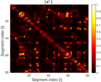
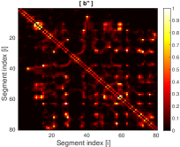
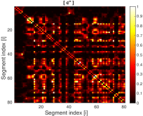
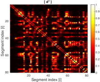
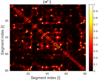
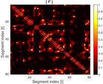
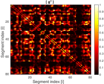
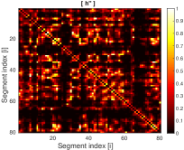
Figure S1: The set of 8 colormaps give the probability of finding the center of mass of segment $i$ and segment $j$ of rings polymers within a distance cutoff of $R^{C}=5a$. The C. Crescentus bacteria ring polymer with $4017$ monomers is considered to be a set of 80 segments with $50$ monomers in each segment. These data provide more structural information of the local arrangements of polymer segments than a stardard pair correlation function $g(r)$ data. Figure (a”),(b”) correspond different runs of a polymer chain with cross links (CL), the locations of CLs correspond to BC-1. Each run stars with different initial configuration. Subplots (c”),(d”) similarly are for different runs with BC-2. The data shown in (e”),(f”) are for different runs with RC-1, and (g”),(h”) for runs with RC-2. This figure gives data from extra runs, corresponding to that of Fig. 2 of main manuscript.

IV Angular Correlations

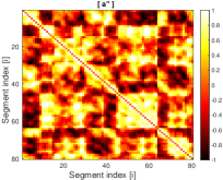
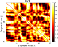
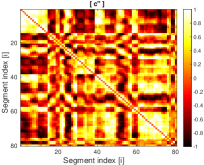
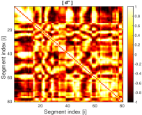
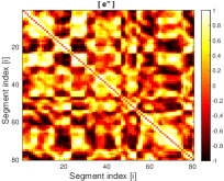
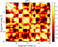
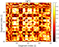
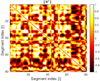
Figure S2: The set of 8 colormaps give the probability of finding the angular correlations between segment $i$ and segment $j$ of a ring polymer. These data provide more structural information of the local arrangements of polymer segments than a standard pair correlation function $g(r)$ data. Figure (a”),(b”) correspond to different runs of a polymer chain with cross links at positions corresponding to BC-1. Each run starts with a different initial configuration. Subplots (c”),(d”) similarly are for different runs with BC-2. The data shown in (e”),(f”) are for different runs with RC-1, and (g”),(h”) for runs with RC-2. This figure gives data from extra runs and correspond to Fig.3 of main manuscript.

V Energy

VI Radial distribution of Segments

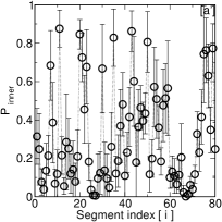
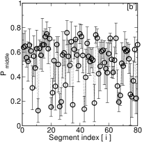
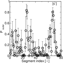
Figure S4: Plot shows the probability $P_{inner},\,P_{middle},\,P_{outer}$ of finding a segment $i$ in the inner, middle and outer regions, respectively, of the polymer for RC-2.

VII Experimental contact-maps

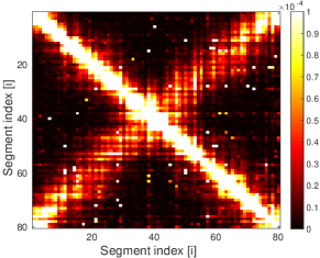
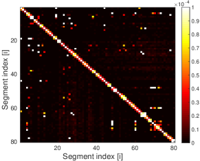
Figure S5: Figure shows colormap obtained from the analysis of Hi-C data and the color represent the interaction frequencies in the experiment. Top colormap is for bacteria C.Crescentus and the bottom colormap is for the E.Coli.

VIII Reasons for differences between colormaps of Fig.2 and Fig.3

Comparing the colormaps of positional and angular correlations in Fig.S1 c”,d” with Fig.S2 c”,d” (or equivalently Fig.2 c,d with Fig.3 c,d) for BC-2, we observe relatively large patches of bright pixels along the diagonal in Fig.S2 c”,d”. The reason for this difference is as follows. the cutoff distance chosen for the calculations in Fig.S1 c”,d” is $R^{C}=5a$; this is nearly equal to the value of $R_{g}$ of the $50$-monomer segments, viz.,$R_{g}\sim{50}^{0.6}a/\sqrt{6}\approx 4.2a$. Thus fewer segments can be accommodated within distance $R^{C}$ from the CM of a particular segment, resulting in small bright patches. In contrast, for angular correlations, we just calculate whether two particular segments lie on the same or opposite side with respect to CM of coil. The relatively large patches of bright pixels in Fig.S2 c”,d” is a consequence of choice of binary values of $\delta^{ij}_{\theta}$ for a particlar microstate. The patterns would be more fuzzy if chose to plot $\langle\cos(\theta^{ij})\rangle$ instead of $\langle\delta^{ij}_{\theta}\rangle$.

IX Construction of 2-D map

To construct the 2-D map, we assumed a spherical globular structure of the DNA-coils and then we use a 3-step procedure in conjunction. Firstly, we know from Fig.1 which segments are to be found primarily in the inner, middle and peripheral region of a globule. Secondly and thirdly, we use the information about which segments are to be found on the radially opposite hemispheres (Fig.3), in tandem with the data about positional correlation given in Fig.2. We use this collective quantitative information to distribute the segments within the schematic diagram of the globule.

X Snapshot from simulation

References

- Le et al. (2013) T. B. K. Le, M. V. Imakaev, L. A. Mirny, and M. T. Laub., Science 342, 731 (2013).
- Joyeux (2015) M. Joyeux, Journal of Physics: Condensed Matter 27, 383001 (2015).
- Cagliero et al. (2013) C. Cagliero, R. S. Grand, M. B. Jones, D. J. Jin, and J. M. O’Sullivan, Nucleic Acids Res. 41, 6058 (2013).
- Lieberman-Aiden et al. (2009) E. Lieberman-Aiden, N. L. van Berkum, L. Williams, M. Imakaev, T. Ragoczy, A. Telling, I. Amit, B. R. Lajoie, P. J. Sabo, M. O. Dorschner, R. Sandstrom, B. Bernstein, M. A. Bender, M. Groudine, A. Gnirke, J. Stamatoyannopoulos, L. A. Mirny, E. S. Lander, and J. Dekker, Science 326, 289 (2009).
- Bickmore and van Steensel (2013) W. A. Bickmore and B. van Steensel, Cell 152, 1270 (2013.).
- Sexton et al. (2012) T. Sexton, E. Yaffe, E. Kenigsberg, F. Bantignies, B. Leblanc, M. Hoichman, H. Parrinello, A. Tanay, and G. Cavalli, Cell 148, 458 (2012).
- Tjong et al. (2012) H. Tjong, K. Gong, Chen, L., and F. Alber, Genome Res. 22, 1295 (2012).
- Dixon et al. (2012) J. R. Dixon, S. Selvaraj, F. Yue, A. Kim, M. H. Y. Li, Y. Shen, J. S. Liu, and B. Ren, Nature 485, 376 (2012).
- Jonathan D. Halverson and Grosberg (2014) K. K. Jonathan D. Halverson, Jan Smrek and A. Y. Grosberg, Reports on Progress in Physics 77 (2014.).
- Dekker et al. (2013) J. Dekker, M. A. Marti-Renom, and L. A. Mirny, Nat Rev Genet. 14, 390 (2013).
- Rob Phillips (2008) J. T. Rob Phillips, Jane Kondev, Physical Biology of the Cell (Garland Science., 2008).
- Rubinstein and Colby (2003) M. Rubinstein and R. H. Colby, Polymer physics (Oxford University Press, Oxford., 2003).
- Maeshima et al. (2010) K. Maeshima, S. Hihara, and M. Eltsov, Current Opinion in Cell Biology 22, 291 (2010).
- Pombo and Nicodemi (2014) A. Pombo and M. Nicodemi, Current Opinion in Cell Biology, 28 (2014.).
- Gilbert et al. (2017) N. Gilbert, Marenduzzo, and Davide, Chromosome Research 25, 1 (2017).
- Fudenberg et al. (2016a) G. Fudenberg, M. Imakaev, C. Lu, A. Goloborodko, N. Abdennur, and L. A. Mirny, Cell Reports 15, 2038 (2016a).
- Mirny (2011) L. A. Mirny, Chromosome Res. 19, 37 (2011.).
- Rosa and Everaers (2008) A. Rosa and R. Everaers, PLOS Computational Biology 4:e1000153 (2008), 10.1371/journal.pcbi.1000153.
- Imakaev et al. (2015) M. V. Imakaev, K. M. Tchourine, S. K. Nechaev, and L. A. Mirny, Soft Matter 11, 665 (2015).
- Barbieri et al. (2012) M. Barbieri, M. Chotalia, J. Fraser, L.-M. Lavitas, J. Dostie, A. Pombo, and M. Nicodemi, PNAS U.S.A. 109, 16173 (2012).
- Fudenberg et al. (2016b) G. Fudenberg, M. Imakaev, C. Lu, A. Goloborodko, N. Abdennur, and L. A. Mirny, Cell Reports 15, 2038 (2016b).
- Goloborodko et al. (2016) A. Goloborodko, J. F. Marko, and L. A. Mirny, Biophysical Journal 110, 2162 (2016).
- Phillips and Corces (2009) J. E. Phillips and V. G. Corces, Cell 137, 1194 (2009).
- Ohlsson et al. (2010) R. Ohlsson, M. Bartkuhn, and R. Renkawitz, Chromosoma 119, 351 (2010).
- Agarwal et al. (2017) T. Agarwal, G. Manjunath, F. Habib, P. Lakshmi, and A. Chatterji, “Role of special crosslinks in structure formation of dna polymer.” (2017), arXiv:1701.05068 .