A Large-scale Dataset and Benchmark for Similar Trademark Retrieval

Abstract

Trademark retrieval (TR) has become an important yet challenging problem due to an ever increasing trend in trademark applications and infringement incidents. There have been many promising attempts for the TR problem, which, however, fell impracticable since they were evaluated with limited and mostly trivial datasets. In this paper, we provide a large-scale dataset with benchmark queries with which different TR approaches can be evaluated systematically. Moreover, we provide a baseline on this benchmark using the widely-used methods applied to TR in the literature. Furthermore, we identify and correct two important issues in TR approaches that were not addressed before: reversal of contrast, and presence of irrelevant text in trademarks severely affect the TR methods. Lastly, we applied deep learning, namely, several popular Convolutional Neural Network models, to the TR problem. To the best of the authors, this is the first attempt to do so.

[table]capposition=top

1 Introduction

A trademark is a recognizable symbol or associated text that identifies products or services of an individual, a business organization or a legal entity from those of others. Registered trademarks are viewed as a form of legitimate property and needs to be protected from brand piracy and trademark infringement. To protect and legalize their trademarks, owners have to register their trademarks in patent offices in many countries. More than 100 million companies are known to exist in local and global markets, and many of them own at least one registered trademark. According to Word Intellectual Property Organization [44], 3 million trademark registrations exist worldwide and trademark applications keep increasing at a rate of 6-8% in recent years.

(a)

(b)

(c)

(d)

(e)

(f)

(g)

(h)

(i)

Figure 1: Sample trademarks and trademark similarities.

Upon application of a new trademark, it needs to be made sure that the new trademark does not imitate or is dissimilar enough from existing trademarks. In most developed countries, organizations like patent offices take the responsibility of protecting trademarks from encroachment. To avoid various infringements, they exclude registration of near-duplicate or intentionally imitated trademarks by manually checking trademarks in the database or by using TR systems. Massive amounts of registration have overwhelmed both manual and automatic operations and reduced service quality of patent offices, which leaves an open space for trademark infringements. What is worse, two mistakenly registered similar trademarks will increase the complexity of handling legal disputation between owners. To ease the burdens of patent offices, a robust automated trademark retrieval (TR) system with intelligent image analyzing techniques is imperative.

However, retrieving all trademark similarities in an efficient and effective way is challenging since:

1. similarity, even when constrained to visual aspects, is eluding since it can occur at many different levels, either visually or semantically – see Figure 1 for some samples. For example, two trademarks can be deemed similar based on the textu(r)al content, the way a line is shaped or placed, or the combinations of such low-level visual content – see Figure 2.

2. similarity is subjective mainly due to the lack of clear criteria for deciding similarity. Visual similarity, especially in the case of trademark similarity, can be influenced greatly by many aspects including education background, religion, hobbies etc.

   Another important factor affecting similarity is the fact that the amount of existing trademarks is tremendous and rapidly increasing, which poses a challenge for the creation of new, substantially different trademark for expressing the same content. This, in time, may lead to a shift in deciding similarity since we may run out of ways to express a meaning.

3. until recently [59], there was no large trademark dataset available to see the challenges of the problem and evaluate the methods. With this paper, we hope to extend our previous work [59] – see Section 1.1 for the details.

4. Available image retrieval methods, which are mostly tailored towards defining similarity in terms of object-related features, are not optimal solutions for trademark retrieval problems, since figures of trademarks mostly incorporate abstract information with various transformations and amounts of detail. In fact, trademark retrieval systems should be equipped with high-level visual capabilities like visual grouping, object recognition, scene/content understanding etc. to be able to handle cases like the ones in Figure 3.

(a) Text only mark

(b) Figure only mark

(c) Figure and text mark

Figure 2: Examples of different trademark types.

1.1 Contributions

In this paper, we focus on trademark similarity defined in terms of visual similarity (see Figure 1 for examples) and skip the conceptual/semantic similarities (see, e.g., [28, 7] for some attempts). Visual similarities of trademarks includes color, shape and texture aspects.

In this work, we extend our previous work [59, 57] and make the following contributions:

• A large-scale dataset and a benchmark: We had already introduced the dataset in our previous work [59]. However, the dataset has been extended with more trademarks and better query samples with which trademark retrieval systems can be tested and compared.

• An analysis of visual features and a baseline: We apply on our dataset many widely-used hand-crafted features (including local and global descriptors based on color, texture and shape – including color histogram, shape context, LBP, SIFT, SURF, GIST, etc.) as well as deep features (AlexNet [31], GoogleNet [56] and VGG-net [52]) that have been shown to perform well on many challenging image recognition tasks. In fact, to the best of our knowledge, this is the first study that has applied deep learning to the trademark retrieval problem. Moreover, we have tested fusion of the best features to see whether they can perform better when combined.

  The performances of the methods reveal that the trademark retrieval problem is very challenging (even for deep learning), and in fact, it should attract more attention than it does in the computer vision and pattern recognition community.

• An analysis of the aspects: We identified that the methods were impeded by the presence of text, or inverse contrast change. To overcome these limitations, we have proposed and tested several methods.

To be more specific, the current paper differs from our previous work [59, 57] in (i) the dataset, and (ii) the methods tested. Namely, the current paper includes deep learning methods, and the improvement of performance of the methods through handling text and contrast change separately.

1.2 Organization

Section 3 introduces the METU trademark dataset. We present our large scale trademark dataset and compare it with other related datasets. Section 4 describes the methods evaluated in this work. These methods are divided into two main groups: traditional hand-crafted features and deep features. In Section 6, the setup and configurations of our experiments are given. Finally, Section 7 concludes the paper with an outline of future work.

(a) WWF logo

(b) IBM logo

Figure 3: Example of how Gestalt principles affect trademark perception.

2 Related Studies

In this section, we discuss the current approaches to trademark similarity, including the manual methods.

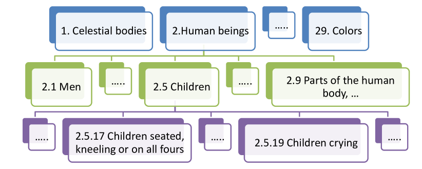
(a) Sample part of Vienna classification categories.

(b) Vienna code: 2.5.19

(c) Vienna code: 2.5.17

Figure 4: Vienna classification categories (a) and sample codes (b-c).

2.1 Checking Trademark Similarity Using Manual Methods

All patent offices still rely on manual effort for evaluating trademark similarity. Such efforts can be fully manual or semi-manual: In a fully manual approach, a human first memorizes a trademark and then skims through the whole collection of trademarks to hopefully spot similarities. In the semi-manual approach, a human first labels the trademarks, retrieves trademarks with the same labels, and visually inspects similarity among the retrieved trademarks.

The accepted standard for the labeling approach is the Vienna classification system, which uses a hierarchy of categories (as displayed in Figure 4a) for labeling the trademarks. For example, the Vienna code (category) for a trademark including human-beings is 2, and 5 as a sub-category for a baby. Based on what the baby is doing, further sub-categories can be attached: e.g., 17 and 19 stand for sitting and crying babies respectively – see Figure 4. When queried with a trademark for similarity, first the trademark is labeled with the Vienna categories, then the trademarks with these categories are retrieved, and similarity is evaluated by an expert using visual inspection.

Although Vienna classification system is practical compared to a fully-manual approach, it bares several disadvantages: (i) The classification process is subjective since the detail of labeling can depend on the observer. (ii) The categories are fixed and not expendable. (iii) It is not possible to describe in words all the content of a trademark, as in the famous saying “a picture is worth a thousand words”.

In short, manual approaches, even sophisticated labeling systems such as the Vienna classification, are (i) unreasonably time-demanding (in the fully-manual case, it takes 3-4 days for a human expert to visually inspect a trademark among approx. 1 million trademarks), (ii) quite error prone since humans are involved in the process, and (iii) unpractical for a trademark system that is rapidly growing with new trademarks. Therefore, automatizing trademark similarity is necessary.

2.2 Checking Trademark Similarity Using Automated Methods

Although patent offices still rely on manual methods, researchers have been working on fully automated methods for similar trademark retrieval for around two decades.

Early attempts applied low/medium level global features, including graphic feature vectors [27], Fourier descriptors [66, 21, 16], image moments [66, 22, 16, 12], Zernike moments [63, 29, 70] as well as simpler and lower-cost shape features such as aspect ratio [16], circularity [16], Rosin descriptor [16], angular radial transform [16], gray level projection [66], gradient orientation histogram [22, 12], wavelets [12], triangle area representation [2, 3] – see Table 1 for an overview. In addition to shape and texture related features, color-feature based approaches have also been applied for trademark retrieval [32, 45, 48, 69, 50].

Jiang et al. [23] pointed out that the aforementioned descriptors do not incorporate geometric information of the extracted features. These descriptors will fail in cases where trademarks match each other at partial parts or unrelated trademarks lead to similar global descriptors. To improve retrieval results, various combinations of these features have been applied. Although there is contrasting evidence [17], effective integration of multiple features has been shown to improve retrieval performance [20, 22].

To improve retrieval results and the partial matching problem, one approach is to segment trademarks to several sub-objects and match trademarks by comparing their part descriptors [4, 5, 6, 15, 16, 17, 22, 35]. However, segmentation is an ill-posed problem, and looking at cases like those in Figure 3, a promising approach should rely on employing perceptual organization and grouping mechanisms similar to Gestalt principles [65]. Some common Gestalt principles like similarity, continuation, closeness, proximity and etc. have already been incorporated into trademark retrieval systems by Eakins et al. [16, 17, 15], Alwis et al. [4, 6], and Jiang et al. [23].

Describing trademarks with global features extracted either from the whole trademark or its parts is time and memory efficient. However, these methods ignore local information, which can be important in addressing partially infringement issues. In order to include local information for addressing partial matching, key-point based methods such as SIFT [30, 64, 36], Harris corners [69], etc. have been tested.

Table 1: Shape-based trademark retrieval methods in the literature.

Group	Approach	Study
Transform- and moment-based shape features	Fourier descriptors	[66, 21, 16]
	Moment variants	[66, 22, 16, 12]
	Zernike moments	[63, 29, 70]
	Wavelets	[12]
	Angular radial transform	[16]
Simple and low-cost shape features	Aspect ratio	[16]
	Circularity	[16, 63]
	Convexity	[16, 70]
	Compactness	[70]
	Eccentricity	[70, 2]
	Distance to centroid	[63]
	Rosin descriptor (triangularity,	[16]
	rectangularity and ellipticity)
	Triangle area representation (TAR)	[2, 3]
Histogram or relation-based shape features	Gray level projection	[66]
	Gradient orientation histogram (edge direction)	[22, 12]
	Shape-context	[50, 49]

2.3 Related Problems: Trademark Detection and Recognition

Trademark detection and recognition are two problems, which are related to trademark retrieval. Trademark detection is the problem of finding all trademarks in a scene. On the other hand, trademark recognition is interested in finding a specific trademark in the scene – see Kesidis et al. [28] for a very detailed survey about these problems.

Kesidis et al. [28] point out that the difference between similarity and matching is subtle but critical to trademark retrieval, since most of the image retrieval methods are designed for exact match rather than detecting similarity. For example, keypoint-based methods rely on having the same keypoints being detected and matched. However, in a similarity problem, two trademarks may not own any common key-points.

3 The METU Trademark Dataset

Existing trademark retrieval studies were conducted on small scale and limited (only consist of special types of logos) datasets, some of which are listed in Table 3. Despite their valuable contributions and prominent results, their practicality, efficiency and reliability can only be confirmed on large scale datasets. For this end, in [59], we shared a very challenging trademark dataset, the METU Trademark dataset, for benchmarking the trademark retrieval problem.

In our previous works [57, 59], we shared the first version of the dataset and conducted several experiments on it. The first version included 930,328 logos, 320 of which belonged to a “query set” for which an expert had identified similar logos already. These query logos are divided into 32 groups. Query logos in the same group are similar to each other. For convenience, here, we name the 930,008 logos as test-set and the 320 query logos as query-set. Figure 5a shows that various types of logos from query-set and test-set. The METU trademark dataset is composed of logos belonging to around 410,000 companies. The test-part of the dataset is provided by the patent office “Grup Ofis Marka Patent A.Ş.” , and “query set” is constructed through collecting and enriching trademark infringement cases appearing in the market. We have performed “cleaning” operations like auto-cropping, filtering corrupted and low-quality trademarks to make our dataset more suitable for academic research.

With this article, we share the second version of the METU trademark dataset. The update includes removal of duplicate logos, and addition of new similar logos in the test-set. As a result, 6,985 logos were removed from the dataset, and the query set is extended to 35 groups, where each group contains around 10-15 trademarks. In total, the query-set contains 417 logos. Figure 5b and 5c are examples of query samples. Detailed comparison of the first and second versions is given in Table 2.

The updated dataset is available on-line for research purposes [58].

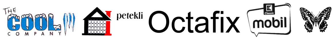
(a) Dataset samples

(b) Example set for similar trademarks

(c) Another example set for similar trademarks

Figure 5: Logo samples from the METU dataset. (a) Arbitrary samples. (b) Sample set for similar trademarks. (c) Another Sample set for similar trademarks.

Table 2: Details of the METU dataset.

Aspect	Version 2	Version 1
# trademarks	923,343	930,328
# query sets	417	320
# unique registered firms	409,675	410,439
# unique trademarks	687,842	690,418
# trademarks containing text only	583,715	589,098
# trademarks containing figure only	19,214	19,387
# trademarks containing figure and text	310,804	311,986
# trademarks with unknown contents	9,610	9,857
# file format	JPEG	JPEG
# Max Resolution	$1,800\times 1,800$(px)	$1,800\times 1,800$(px)
# Min Resolution	$30\times 30$(px)	$30\times 30$(px)

3.1 Comparison with Other Datasets

A comparison with the available datasets is provided in Table 3. To the best of our knowledge, the METU trademark dataset is the largest, organized and challenging publicly available dataset. Compared to other datasets used in previous studies, the METU TR benchmark dataset is very realistic, both at size and types of the trademarks aspects.

There is also a raw dataset, called USTPO Trademark application bulk dataset, which also contains millions of trademarks. However, before using it in trademark retrieval, it needs substantial amount of preprocessing (for removing duplicates, non-cropping cases and getting additional useful information like types, texts of trademarks, etc.).

Table 3: A comparison of trademark datasets available in the literature.

Dataset	Number of	Requires	Image	Image	Ref.
	logos	preprocessing?	type	size (px)
UM	106	No	BW	various	[40]
MPEG7 CE2B	3,621	No	BW	-	[62]
Wei et al.	1,003	No	BW	$200\times 200$	[63]
$Alwis$ et al.	210	No	BW		[4]
$Alwis$ et al.	1,000	No	BW	-	[6]
$abdel$ et al.	63,718	No	BW	-	[1]
MPEG7 CE2B	1,400	No	BW	256$\times$256	[46]
MPEG7	3,000	No	BW	-	[23]
Jain et al.	1,100	No	BW	$200\times 200$	[22, 11]
UKTR	10,745	No	BW	-	[15]
Leung et al.	2,000	No	BW	-	[35]
Her et al.	2,020	No	RGB	$64\times 64$	[20]
USPTO	$\sim$1,500,000	Yes	RGB	various	[18]
METU	923,343	No	RGB	various	[59]

4 Methods

In this section, we introduce the visual features tested on our dataset. We group the features into two broad categories based on whether they are hand-crafted or learned using deep learning methods. Moreover, we present how we can fuse the best features to obtain better results.

4.1 Hand-crafted Features

Hand-crafted features are designed based on “expert” knowledge and experience on the problem at hand. These designed features try to capture different aspects of what is available in an image. These aspects include color, shape, texture etc., which can be analyzed locally or globally.

In the following, we first introduce color features, then discuss global shape and layout-based features. After that, we will describe the key-point features, which are good at capturing partial similarity.

4.1.1 Color Feature: Color Histogram

Color is a widely-used integral property of trademarks, giving them an extra dimension for expressing information. As pointed out by Her et al. [20], color schemes of trademarks are not only attractive to customers, but also protected through additional registration processes [28].

Color similarity of trademarks is determined usually by comparing their color histograms. Color histogram is a short summary of the distribution of color in the trademarks. It is translation and scale invariant (when normalized properly). However, most of the time, color is not sufficient to identify similarity, which is mostly due to shape similarities; therefore, color is generally used together with other features [32, 45, 48, 69, 50].

The efficiency and effectiveness of the color histogram method is dependent on the color space, quantization, distance measures and normalization methods used. In our previous work [57], we experimented with two most widely used color spaces: RGB and HSV.

Due to these crucial differences between the two color spaces, two different quantization methods are used: The RGB color space is uniformly quantized into 64 or 512 different colors by dividing each of its color channels to 4 or 8 parts. However, our choice of quantizing the HSV color space is not uniform (to see the necessity for this better: looking at the 3D cylindrical model of the HSV color space, one finds that the bottom part is black while the top part is colorful. These colors in the black region make little difference to human eyes [34]. According to this observation, nonuniform quantization methods have been proposed [34, 19, 55].

As to the distance measures and normalization methods, we chose five different distance metrics: Euclidean, Cosine, Intersection, Quadratic, and Manhattan distances, and L1 and L2 normalizations – see A and B for a definition of distance metrics and the normalization methods.

As shown in Figure 6, we selected the best parameter settings on a small subset of our dataset. This subset includes 600 colorful trademarks in 10 different colors: red, green, blue, cyan, yellow, pink, black, gray, orange and brown. From this investigation, we found the following setting to perform best: HSV color space with 72 bin normalization (same as [34]), intersection distance method, and L1 normalization return the best retrieval results. In the rest of the article, we adopt these settings for the color feature.

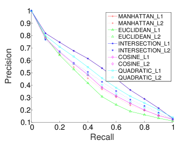
(a) The PR graph of RGB color histograms of 64 bins

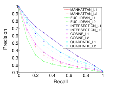
(b) The PR graph of RGB color histograms of 512 bins

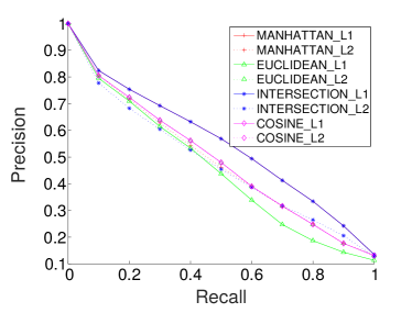
(c) The PR of HSV color histograms of 36 bins

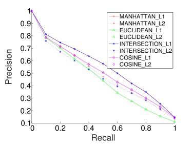
(d) The PR of HSV color histograms of 72 bins

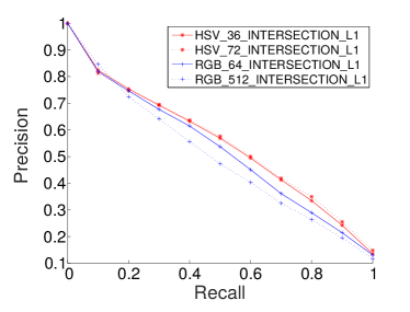
(e) The comparison of outstanding schemes from (a-d)

Figure 6: The effects of the parameters in color-based trademark retrieval in a small colorful subset of the METU dataset, grouped by the utilized normalization scheme and color space. (a-d) The results of RGB color histograms of 64 and 512 bins and HSV color histograms of 36 and 72 bins, compared for various distance metrics. (e) A comparison of the best overall results. The numeric prefixes in the legend entries denote the number of quantization bins, while the string suffixes indicate the utilized distance metric and normalization.

4.1.2 Texture Feature: Local Binary Patterns (LBP)

Texture is an important cue in evaluating similarity of trademarks, and for representing textural content of an image, Local binary patterns (LBP) [41, 42] is a popular, simple and efficient choice. LBP extracts structural patterns from images by comparing the intensity of a pixel with $N$ neighbors around it in a certain radius. Patterns are outcomes of comparisons in the $N$ bit binary number format. The statistics of occurrences of each pattern in an image is then expressed as a $2^{N}$-bin vector. Given the LBP vectors of two images (trademarks), their textural similarity can be queried using the distance between their LBP vectors.

Ojala et al. [41] generalized LBP with the following expression,

$$LBP_{P,R}=\sum_{p=0}^{P-1}{s(g_{p}-g_{c})2^{P}},$$ (1)

where $P$ is the count of neighbors in a circle with radius $R$, and $g_{p}$ and $g_{c}$ are intensities of pixel $p$ and the center pixel respectively, and $s(x)$ is equal to $0$ when $x$ is more than or equal to $1$, otherwise $0$.

The rudiment LBP method could achieve rotation invariance and robust discrimination ability with some modifications, such as bit-wise shifting and ‘uniform’ operations [42]. Similar to the color histogram method, the performance of the LBP method is dependent on the selected distance metric and normalization method. Figure 7 displays the effect of the different settings, which shows the best LBP configuration to be the original LBP method with the cosine distance metric and L1 normalization. Therefore, we will adopt these settings for LBP in the rest of the article.

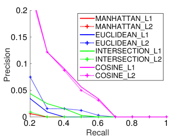
(a) The PR graph of $LBP_{P,r}$

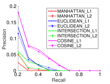
(b) The PR graph of $LBP_{P,r}^{ri}$

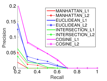
(c) The PR graph of $LBP_{P,r}^{u2}$

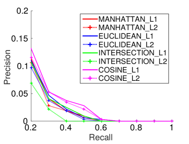
(d) The PR graph of $LBP_{P,r}^{riu2}$

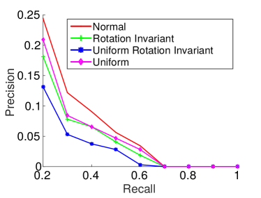
(e) The comparison of outstanding schemes from (a-d)

Figure 7: Performance of different LBP variants on the METU dataset. (a-d) The results of $LBP_{P,r}$, $LBP_{P,r}^{ri}$, $LBP_{P,r}^{u2}$, $LBP_{P,r}^{riu2}$. (e) A comparison of the best overall results. In legends of (a-d), the string suffixes indicate the utilized distance metric and normalization type.

4.1.3 A Global Feature: GIST

The GIST descriptor is initially designed for scene recognition [43]. It describes objects with spatial envelope properties (a very low dimensional representation of the scene): the degree of naturalness, openness, roughness, expansion and ruggedness. These properties are computed by using the principal components of the global energy spectrum and the spectrogram. Since the descriptor uses only the mentioned spatial envelope properties, it projects images into a low dimensional feature space. This makes GIST a very compact and efficient descriptor for a global representation of an image.

Douze et al. [14] used GIST for large scale copyright detection. They found that GIST outperforms the most commonly used model, i.e., BoVW with local descriptors like SIFT, when searching duplicate images from a very large scale image dataset. We expect that GIST descriptor can be useful in trademark retrieval as well since it is known to be good at capturing the layout of a figure.

4.1.4 Bag of Visual Words (BoVW)

The scaling problem is the bottle neck of large scale trademark retrieval, especially when methods extract multiple high-dimensional features from images as methods introduced in the following part. Storing and comparing tremendous key-point features extracted from large scale dataset is very challenging. Therefore, the method of bag of visual words (BoVW) [54] is adapted. In this approach, each feature is expressed with their unique cluster id, which is obtained by clustering all features to $k$ different classes. This BoVW model not only shrinks the feature spaces, but also grants the computational efficiency through applying the TF-IDF (term frequency-inverse document frequency) [10] and inverted file structures [54]. Through applying this model, high dimensional features space are mapped into vectors whose similarity is calculated with cosine vector distance metric in this study.

4.1.5 Shape Context

The main content of images, shapes, makes substantial impression on customers [20]. It is, therefore, one of the most significant aspects considered for judging similarity.

A robust shape feature is critical to trademark retrieval. Yang et al. [67] suggest that a robust shape feature should include most of the following properties: identifiability, translation, rotation, scale, affine and occlusion invariance, noise resistance, statistical independence, reliability. The shape context method proposed by Belongie et al. [9] is known to be a suitable shape descriptor, satisfying most of the properties aforementioned. The shape context of a shape is spatial distributions of all sample points to each sample point from it. The deformation energy necessary for matching shape contexts is the similarity degree of shapes.

The shape context of a shape is generated through the following steps: (1) Uniformly sample $n$ points from inner and outer outline of the shape. (2) Assign a log-polar histogram to each sample point. A sample log histogram, in which radius bins $\theta$ is 5 and angle bins $logr$ is 12, is shown in Figure 8. (3) According to the allocation of sample points on each log-histogram, generate $n$ vectors of shape context.

(a) Logo of NIKE

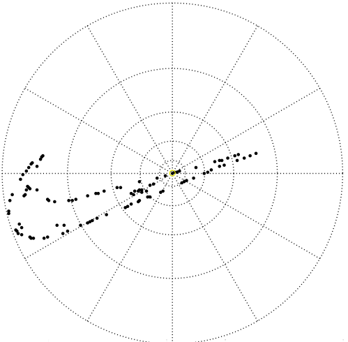
(b) a polar histogram of a point on NIKE logo

Figure 8: A polar histogram of a sample logo (Adapted from [57]).

Computing the deformation energy of shape contexts of million shapes is costly. Approximate solutions have been developed for this purpose. For example, Mori et al. [38] proposed two different approximation approaches: representative shape-context and shapeme histogram descriptor. The shapeme histogram method is similar to the BoVW method. It applies vector quantization to all descriptors as shown in Figure 9. With this approach, the shape context becomes more efficient in terms of time and memory aspects. What is more, Rusino et al. [49] achieved further scalability through organizing shapeme histogram descriptors by a local-sensitive hashing indexing structure for searching similar descriptors in a sub-linear time. In this article, we will employ the shape-context descriptor with the BoW model with a dictionary size of 10,000 (this is decided empirically).

(a) NIKE

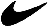
(b) NEWPORT

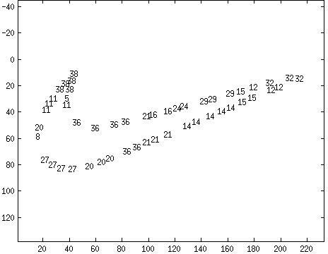
(c) Shape-context of NIKE logo

(d) Shape-context of NEWPORT logo

Figure 9: Shapeme of sample logos (Adapted from [57]).

4.1.6 Keypoint-based Features

If two trademarks are similar, they should be composed of similar key-points. To extract key-point descriptors from an image, the first step is detection: One of the most popular methods for this purpose, SIFT, takes as key-points the intensity changes overlapping in multiple scales in a multi-scale filtered representation of an image. While, for speeding up the detection process, SURF applies a Hessian-matrix-based blob detector to find key-points.

After detection, the second step is the description of the visual content at and around keypoints. Key-point descriptor methods generate a description of a key-point usually from the distribution of gradients and orientation of its nearby pixels.

In this study, we evaluate the most popular key-point descriptors: SIFT [37], SURF [8], and HOG [13]. In several studies [30, 64, 36], these features have been already applied for trademark retrieval.

Triangular SIFT: Despite the fact that SIFT is an effective, stable and robust descriptor, it is not recommended for large scale datasets because of its computational complexity. To scale up SIFT, the local geometry information is usually incorporated.

One such promising attempt, owing to Kalantidis et al. [26], showed that grouping SIFT features at the same scale as triplets and comparing only triplets of SIFTs at the same scale at the matching phase both improves the accuracy and running-time.

4.2 Learned Features Using Convolutional Neural Networks (CNN)

To the best of our knowledge, this is the first study using deep learning for trademark retrieval. Deep learning (networks) relies on finding an end-to-end mapping directly from the raw input to the required output, whereby the best representation for the problem at hand is obtained from the data directly, leading to distributed, compositional, hierarchical representations.

One of the prominent methods in deep learning is Convolutional Neural Networks (CNNs), which exploit local connectivity and weight sharing mechanisms (see, e.g., [33]). CNNs mainly learn filters for convolution operation at different layers and scales, together with complementary operations like non-linear transformation, pooling (down-sampling) etc. These filters are trained using back propagation for various problems such as classification, detection and recognition.

In this work, we evaluated the widely used pre-trained networks, namely AlexNet [31], VGGNet [52], and GoogLeNet [56] – see Table 4 for a comparison of the architectures. We extracted features from trademarks through these models, then compared these features with cosine vector distance.

We have also trained two different comparatively shallow denoising autoencoders [60]. These two autoencoders use $3\times 3$ convolutional kernels, following the work of [52]. The encoder structure of the autoencoders, $ae^{1}$ and $ae^{2}$, are [16 ($3\times 3$), 8 ($3\times 3$), 8 ($3\times 3$)] and [128 ($3\times 3$), 64 ($3\times 3$), 64 ($3\times 3$)] respectively – see also Table 4.

Table 4: A comparison of the deep networks. For the number of layers, only weighted layers are counted. In the architecture descriptions, I represents input; C, convolution layer; P, pooling layer; D, dropout layer; F, fully connected layer; and N, inception network described in [56].

Network	# of	# of	Feature	Overall
	layers	parameters	dimension	architecture
AlexNet [31]	8	61M	4,096	$I-[CP]^{2}-C^{2}-[CP]-F^{3}$
VGGNet16 [52]	16	138M	4,096 (FC7)	$I-[CCP]^{2}-[CCCP]^{3}-F^{3}$
VGGNet16 [52]	16	138M	1,000 (FC8)	$I-[CCP]^{2}-[CCCP]^{3}-F^{3}$
GoogLeNet [56]	22	6.9M	1,024	$I-[CP]-[CCP]-N^{9}-P-F$
Autoencoder ($ae^{1}$)	8	4,963	288	$I-[CP]^{3}-[CU]^{3}-C$
Autoencoder ($ae^{2}$)	8	200,899	8,192	$I-[CPD]^{3}-[CU]^{3}-C$

4.3 Summary

Overall, we have selected a wide range of features representing different aspects of content in trademarks, both hand-designed and learned from data directly. These features have different advantages and disadvantages, as shown in Table 5, which indicates their fusion might perform better than the individual methods.

Table 5: Comparison of the feature extraction methods.Robustness means robustness to translation, scaling, rotation, and occlusion, and efficiency pertains to time and memory efficiency.

Algorithm	Shape	Color	Texture	Layout	Partial	Efficiency	Robustness	Type
					matching
Color	-	$*****$	-	-	-	$****$	$*$	Global
LBP	-	-	$****$	-	-	$****$	$***$	Global
GIST	$***$	$***$	$***$	$****$	-	$****$	$**$	Global
SHAPEMES	$****$	-	-	$***$	$***$	$***$	$***$	Local
HOG	$**$	-	$**$	-	$***$	$**$	$***$	Local
SIFT	$**$	-	$**$	-	$****$	$*$	$***$	Local
SURF	$**$	-	$**$	-	$****$	$**$	$***$	Local
DCNN	$****$	$***$	$***$	$***$	$***$	$**$	$****$	Local

5 Enhancing and Fusing Features

We noticed that the overall performance of some features could be improved by (i) leveraging contrast change and removing text, which is irrelevant for trademarks not including text, and (ii) fusing the features, combining their advantages.

5.1 Detecting and Removing Text in Trademarks

Text is a misleading element for retrieval if the query logo does not include any text. Text in trademarks leads to many keypoints and features, which significantly affect the overall matching performance – see Figure 10. If the query logo includes text, a good strategy is to recognize the text and evaluate similarity based on the recognized text.

For locating text in trademarks, we use a state-of-the-art method proposed by Neumann et al.  [39], which performs real-time text localization by detecting characters by using the Extremal Region (ER) detector, which is robust and stable to illumination, blur, and color and texture variation – see Figure 11 for some results.

(a)

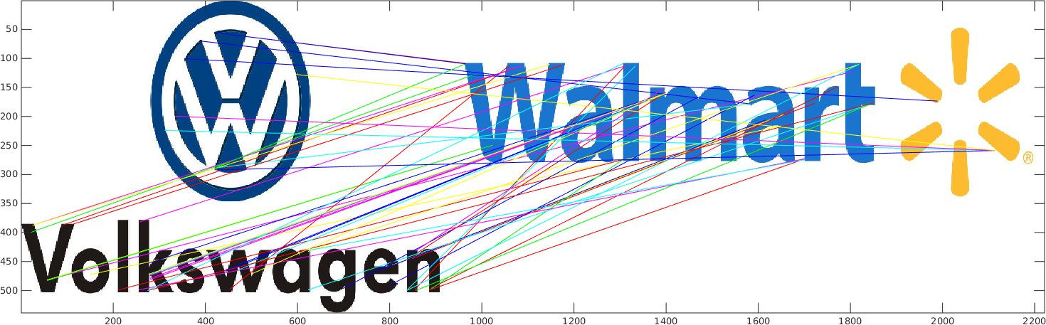
(b)

Figure 10: Example of the influence of characters on key-point based detection (shown for the SIFT features).

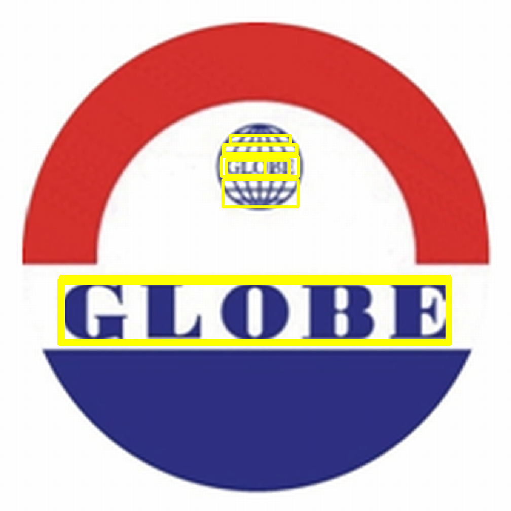
(a)

(b)

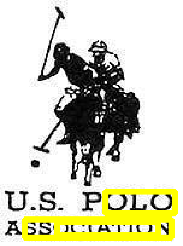
(c)

(d)

Figure 11: Text detection results on sample trademarks (detection shown in yellow) using the method by Neumann et al. [39].

5.2 Contrast Enhancement

Key-point feature descriptors like SIFT are sensitive to contrast change, which causes TR systems to be ignorant to infringements that include a different contrast change – see Figure 12 for examples. Extensions of SIFT, namely Orientation-Restricted SIFT (OR-sift) and GOM-SIFT presented in [61, 68], are made robust to this contrast issue. GOM-SIFT achieves this by restricting orientation values of each feature between $0^{\circ}$ and $180^{\circ}$ for increasing the performance against contrast cases. GOM-SIFT leads to improvement though sacrificing rotation invariance. To keep contrast robustness with rotation invariance, Vural et al.  [61] proposed OR-SIFT, which merges directions who are $180^{\circ}$ apart. For this reason, we employ OR-SIFT in this article. See Figure 12 for results of OR-SIFT key-point comparisons on trademarks having contrast differences.

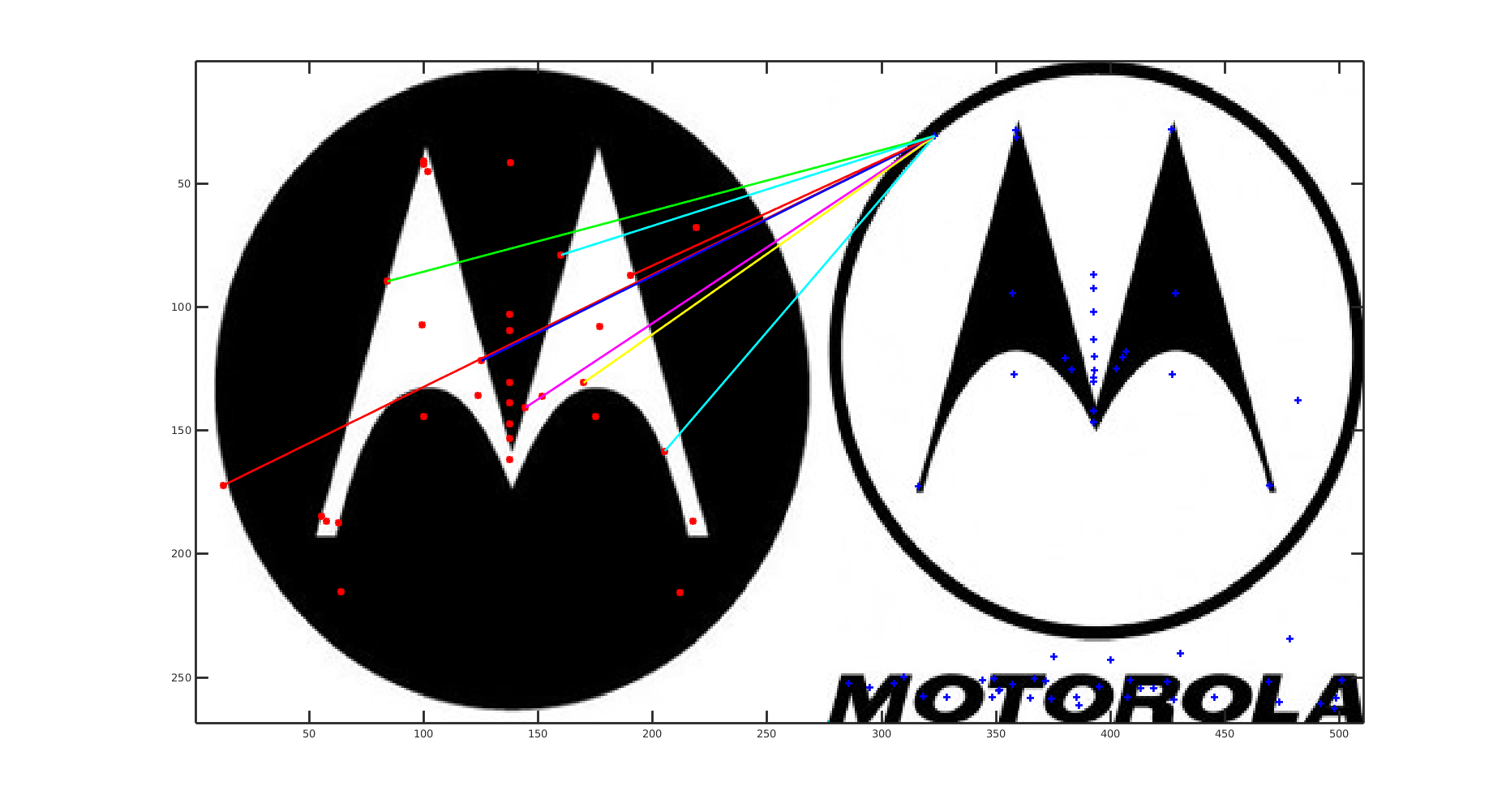
(a) SIFT

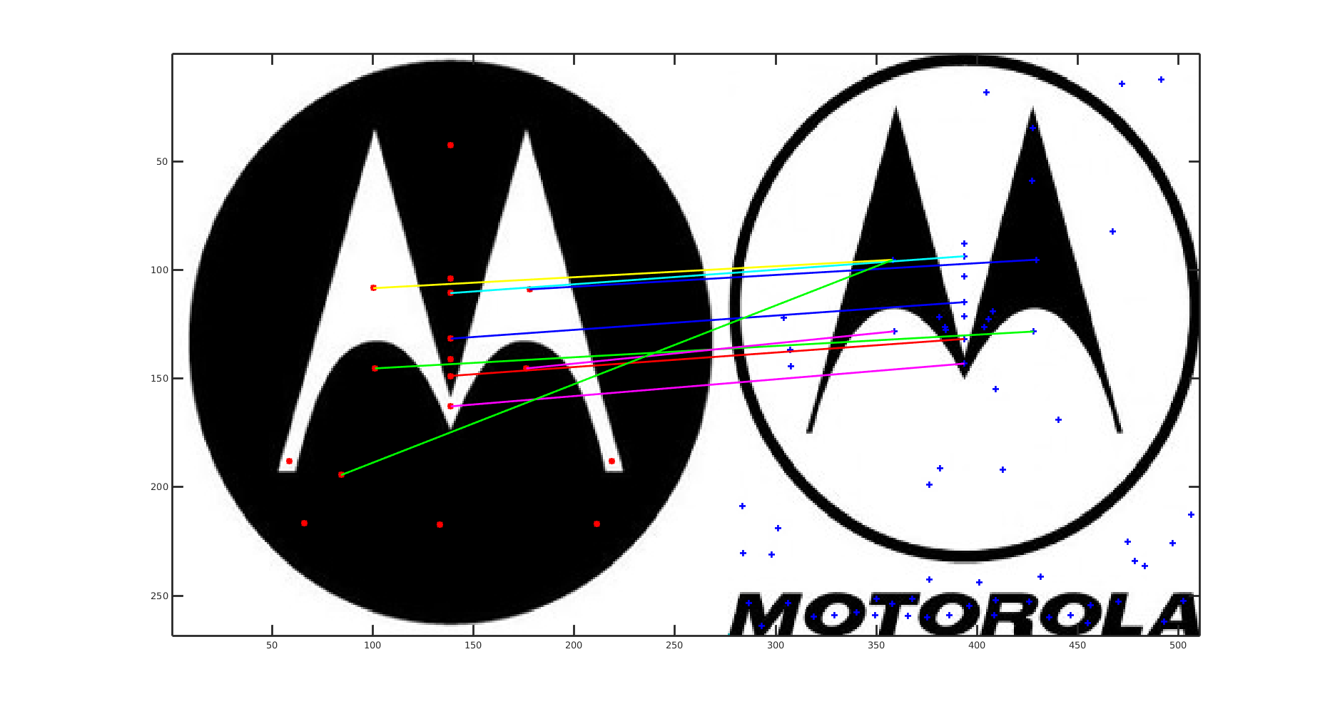
(b) OR-SIFT

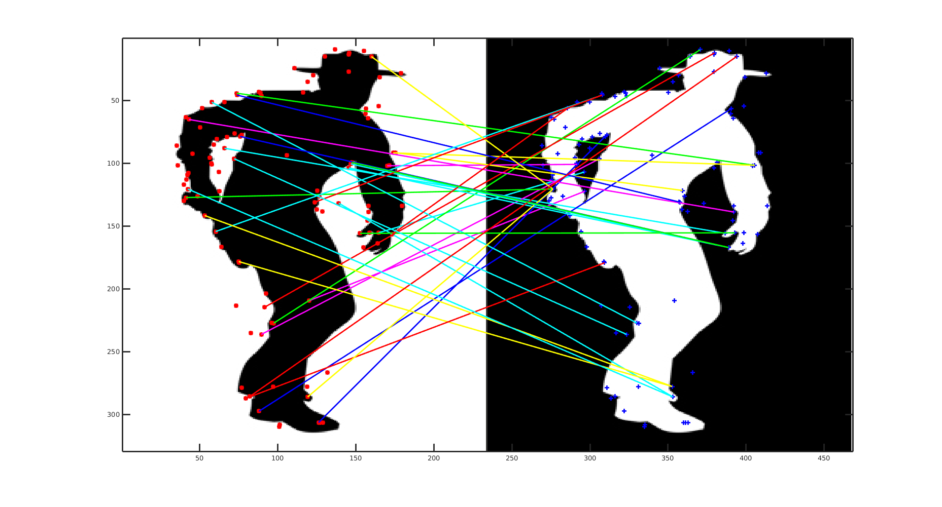
(c) SIFT

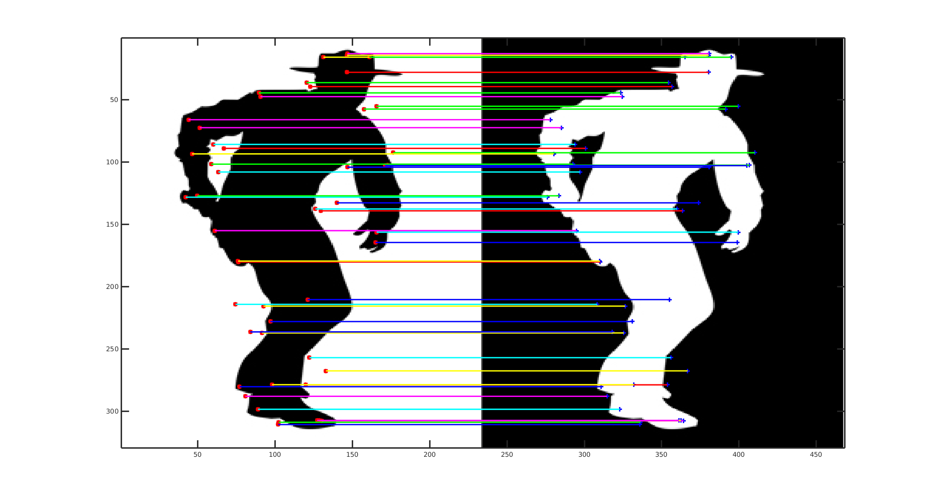
(d) OR-SIFT

Figure 12: Matching images with different contrast changes using SIFT and OR-SIFT[61]. In (a-b), similarity between the trademarks is missed using naive SIFT. In (c-d), a modification of SIFT, OR-SIFT, captures the similarity despite contrast change. Lines are colored randomly only for the sake of visibility.

5.3 Fusion of Features

In trademark retrieval, fusion of features has been applied successfully already [48, 47, 63, 70, 17]. In this study, we have also fused the best performing methods. The fusion method we have applied is Inverse Rank Position (IRP) [25]. It takes inverse of the sum of inverse of similarity ranks.

$$IRP(q,i)={1}/{\sum_{j}^{n}{\frac{1}{rank_{j}}}},$$ (2)

where $j$ represents the $j^{th}$ feature, $q$ is query image, $i$ is $i^{th}$ image.

6 Experiments and Results

In this section, we first introduce the experimental setup, the evaluation method, and then the results with an analysis.

6.1 Experimental Setup

Most of the experiments are conducted on a PC with an Intel i7-4770K 3.50GHz CPU with 32GB DDR3 memory, and a GeForce GTX 760 graphics card. However, we used the Tesla K40 GPU card for developing autoencoder models.

Our main experiment flow is visualized in Figure 13.

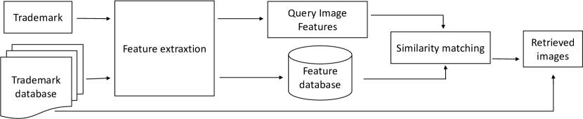
Figure 13: The overall view of how the experiments are performed.

6.2 Evaluation Method and Metrics

As discussed in Section 3, the dataset includes 45 query groups, and in each group there are around 10-15 logos for which similarities have been identified by an expert. For each image in the query set, we “inject” the other images in the query group into the test-set, apply the trademark retrieval method and look at the rank of the logos that have been injected.

For evaluating the retrieval performance, we use precision-recall (PR) graphs, and average ranks of the “injected” known trademarks as performed in the CBIR literature. Precision and recall are defined as follows:

$$Precision=\frac{\emph{No. of relevant retrieved Trademarks }}{\emph{No. of retrieved Trademarks}},$$ (3)

$$Recall=\frac{\emph{No. of relevant retrieved Trademarks}}{\emph{No.of relevant Trademarks}}.$$ (4)

A PR graph offers an intuitive comparison of the retrieval ability of a set of methods for various levels of sensitivity. Besides PR, we use average rank and normalized rank for evaluating ranking ability of the methods. The normal rank metric returns actual average ranks of relevant logos (following the notation and the definition by Sivic & Zisserman [54]):

$$Rank=\frac{1}{N_{rel}}\sum\limits_{i=1}^{N_{rel}}{R_{i}},$$ (5)

where $N_{rel}$ is the number of relevant images for a particular query image, $N$ is the size of the image set, and $R_{i}$ is the rank of the $i^{th}$ relevant “injected” image. In contrast, the normalized rank metric returns a score for evaluating the robustness of the retrieval method:

$$\widetilde{Rank}=\frac{1}{N\times N_{rel}}\left(\sum\limits_{i=1}^{N_{rel}}{R_{i}-\frac{N_{rel}(N_{rel}+1)}{2}}\right).$$ (6)

Average rank ranges from $1+\frac{N_{rel}}{2}$ to $N-\frac{N_{rel}}{2}$ s.t. the smaller the rank is, the better the performance is. In contrast, the normalized rank measure lies in the range $[0,1]$. Zero ($0$) corresponds to the best performance, and $0.5$ to random performance. These two ranking scores capture a global view of retrieval ability of the methods. However, in our experiments, methods exhibit different retrieval performances to different queries. In order to capture this, we also visualize the ranking results of all queries as a graph.

Last but not the least, in the ranking process, we realized that tie cases may occur due to same similarity scores when descriptors failed to extract sufficient information from the trademarks. For resolving the tie cases, the average of original ranks is used in the following ranking results (similar to [51, 24]).

6.3 Results

In this section, we analyze the methods in terms of performance and efficiency. Sample queries are provided at the following page: http://kovan.ceng.metu.edu.tr/~osman/dataset_webpage/query.html.

6.3.1 Precision-Recall and Average Rank Results

Table 6: Comparison of the results of the traditional individual methods.

Algorithm (id)	BoW	Without	Average	Normalized
	cluster	text?	rank	average rank
Color ($cl$)	-		369,598.3 $\pm$ 161,895.1	0.400 $\pm$ 0.175
LBP ($lp$)	-		254,971.8 $\pm$ 131,399.5	0.276 $\pm$ 0.142
GIST ($gs$)	-		234,087.1 $\pm$ 159,585.2	0.254 $\pm$ 0.173
SHAPEMES ($sh$)	10k		203,408.2 $\pm$ 171,317.4	0.220 $\pm$ 0.186
HOG ($hg$)	10k		242,166.1 $\pm$ 118,686.6	0.262 $\pm$ 0.129
SIFT ($si^{1}$)	10k		164,837.7 $\pm$ 133,932.5	0.179 $\pm$ 0.145
SIFT ($si^{2}$)	999		192,881.1 $\pm$ 144,359.4	0.209 $\pm$ 0.156
SIFT ($si^{3}$)	9		321,268.8 $\pm$ 132,487.4	0.348 $\pm$ 0.143
TRI-SIFT ($ts$)	9		298,744.3 $\pm$ 148,279.1	0.324 $\pm$ 0.161
OR-SIFT ($os$)	10k		175,482.6 $\pm$ 139,185.6	0.190 $\pm$ 0.151
SIFT ($si^{4}$)	10k		141,840.9 $\pm$ 117,705.3	0.154 $\pm$ 0.127
SURF ($su$)	10k		191,304.1 $\pm$ 139,696.4	0.207 $\pm$ 0.151

We display the rank results of the hand-crafted features and the CNN features in Tables 6 and 7 respectively. These tables show mean and standard deviation values of $Rank$ and $\widetilde{Rank}$ of the implemented methods. The best method should have the smallest $Rank$ and $\widetilde{Rank}$ values. Figures 14, 16, 18 and 20 show the PR graphs. In these figures, each PR curve includes also a zoomed version for the sake of better visibility. Although rank results and PR curves indicate the overall performance of the method, they fail to highlight a method’s performance on individual queries. For this end, we provide a display of performance on individual queries in Figures 15, 17, 19 and 21. In an individual rank graph, the X-axis is the query id. The length of X-axis is 417, since we have 417 queries. The Y-axis is rank value of the each queries. When a query is given, the optimal method will return expected results with a priority. Therefore, the marks of the optimal method will be very close to X-axis, and the density of the zoomed version will be high at nearby the X-axis.

From Table 6, we see that the worst retrieval result is due to the color histogram method. This is expected since color is not sufficient for providing an overall judgment for trademark similarity. What is worse, half of the dataset are text-only trademarks, and mostly black and white. However, as shown in Figure 17, we see that, although color is not sufficient, it is necessary for determining similarity for some trademarks: In fact, in some cases, color histogram results are very close to the X-axis, which means it works well on some of the queries.

Looking at the performance of the hand-crafted features, we see that the performance of global-features (LBP, GIST) are more or less the same. However, based on our experience gained by visualizing query results, we found that the GIST method is better at capturing layout similarity, while the LBP performs better on texture similarity (not reported here). What is more, we can see that BoVW model based local feature methods yield better results than the global features. Among them, SIFT without text features ($si^{4}$) perform best. SIFT with 10k visual words is the second performing method. Surprisingly, TRI-SIFT does not perform better than the original SIFT since most trademarks yield insufficient number of keypoints for TRI-SIFT to make difference. This is in contrast to our previous results [57, 59], which is due to the fact that we handle the tie cases differently in this paper (following the literature - [51, 24]), and that TRI-SIFT produces a large number of tie cases. Similarly, OR-SIFT does not outperform the original SIFT neither; however, Figure 15 suggests that it is better than SIFT in certain queries.

Table 7 lists the $Rank$ and $\widetilde{Rank}$ performance of the CNN based methods. We can see that their performances are far better than those of the hand-crafted features. Among the individual methods, the features extracted from FC7 layer of VGG-Net16 returns the best result. This is expected since VGG-Net is known to have learned more generic representations than GoogleNet or AlexNet (see, e.g., [53]). However, Figure 19 shows that these models perform differently on individual queries, for example, AlexNet outperforms other networks on certain queries.

6.3.2 Fusion Results

We have selected the best performing methods under each category and fused them. Looking at the fusion results in Table 8, fusion improves the performance substantially. With a simple and efficient fusion method like IRP, we observe a clear improvement in both hand-designed features and learned features. In fact, fusing together the fusion of hand-crafted and deep features (denoted $f^{3}$ in the Table 8) yields the best performance among the tested methods. However, looking at the precision and recall values in Figures 16, 18 and 20, we see that fusion leads to slight decrease in precision. This is mainly due to the fact that fusion discovers similar logos not anticipated by us.

Table 7: Comparison of the results of the CNN methods.

Net	Layer	Size	Average rank	Normalized
				average rank
AlexNet ($ax^{1}$)	FC7	4,096	103,549.2 $\pm$ 157,877.9	0.112 $\pm$ 0.171
AlexNet ($ax^{2}$)	Pool5	9,216	125,300.9 $\pm$ 157,739.5	0.136 $\pm$ 0.171
GoogLeNet ($gl^{1}$)	77S1	1,024	108,662.5 $\pm$ 127,619.1	0.118 $\pm$ 0.138
VggNet16 ($vg^{1}$)	Pool5	25,088	88,829.1 $\pm$ 112,370.7	0.096 $\pm$ 0.122
VggNet16 ($vg^{2}$)	FC7	4,096	79,538.5 $\pm$ 98,961.3	0.086 $\pm$ 0.107
VggNet16 ($vg^{3}$)	FC8	1,000	98,716.9 $\pm$ 100,910.4	0.107 $\pm$ 0.109
Autoencoder ($ae^{1}$)	Last	288	287,884.8 $\pm$ 157,787.7	0.312 $\pm$ 0.171
Autoencoder ($ae^{2}$)	Last	8,192	209,029.0 $\pm$ 142,507.9	0.226 $\pm$ 0.154

Table 8: Comparison of the results of fusions.

Fusion	Method	Items	Average rank	Normalized
				average rank
Fusion ($f^{1}$)	IRP	$cl,lp,sh,gs,si^{1},su$	96,545.1 $\pm$ 100,474.7	0.105 $\pm$ 0.109
Fusion ($f^{2}$)	IRP	$ax^{1},gl^{1},vg^{2}$	73,239.0 $\pm$ 11,7881.2	0.079 $\pm$ 0.128
Fusion ($f^{3}$)	IRP	$f^{1},f^{2}$	56,844.1 $\pm$ 87,794.1	0.062 $\pm$ 0.095

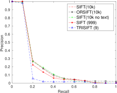
(a) Original

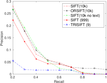
(b) Zoomed

Figure 14: Precision-recall results of SIFT and its variants.

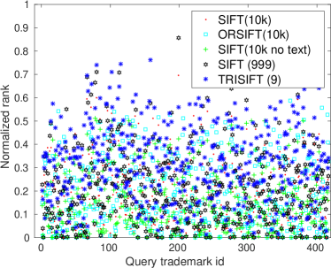
(a) Original

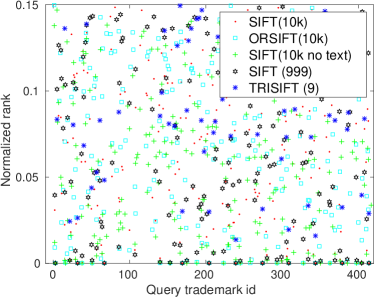
(b) Zoomed

Figure 15: Normalized average ranking results of SIFT and its variants.

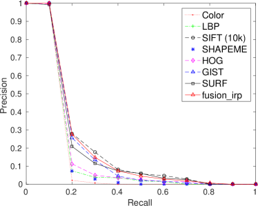
(a) Original

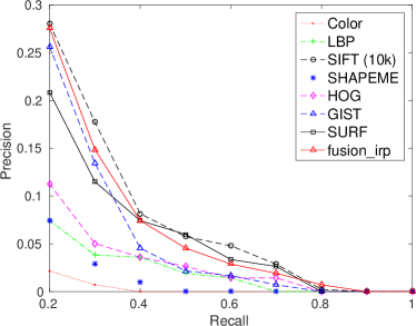
(b) Zoomed

Figure 16: Precision-recall results of hand-crafted features. (a) Original view, (b) Zoomed view.

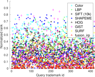
(a) Original

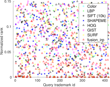
(b) Zoomed

Figure 17: Normalized average ranking results of hand-crafted features. (a) Original view, (b) Zoomed view.

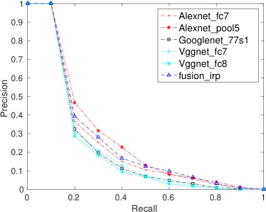
(a) Original

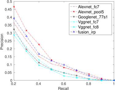
(b) Zoomed

Figure 18: Precision-recall results of DCNN features. (a) Original view, (b) Zoomed view.

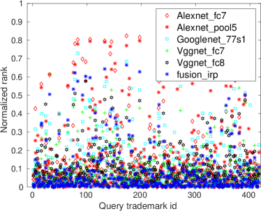
(a) Original

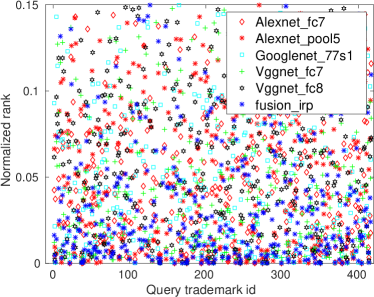
(b) Zoomed

Figure 19: Normalized average ranking results of DCNN features.(a) Original view, (b) Zoomed view.

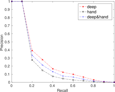
(a) Original

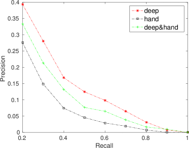
(b) Zoomed

Figure 20: Precision-recall results of fusion features. (a) Original view, (b) Zoomed view.

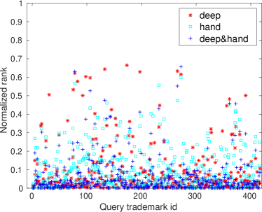
(a) Original

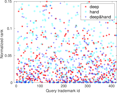
(b) Zoomed

Figure 21: Normalized average ranking results of fusion features.(a) Original view, (b) Zoomed view.

6.3.3 Time and Memory Aspects

Tables 9 and 10 compare running time and memory aspects of the tested methods respectively. Running time measures three phases: feature extraction, feature processing, and ranking. CNN features have the fastest feature extraction phase because of GPU parallelization. Feature processing time is the extra time we spend for steps like vectorization, text removal, and feature grouping etc. The ranking time contains similarity calculation and sorting times.

In our experiments, each query is compared with all other trademarks in the dataset, and the trademarks are sorted by similarity for retrieving the top $m$ results. Looking at Table 9, we see that the maximum time for querying a trademark in our dataset is about 17 seconds. Although this is a realistic figure, it can be improved even further since our tests were conducted in MATLAB. Moreover, we see opportunities for further improvement by parallelizing the feature matching phase.

In large-scale trademark retrieval, the descriptor size becomes an important factor. Table 10 compares the size of the descriptors as a measure for the require memory. We see that the key-point based methods have large descriptor sizes whereas global features have smaller sizes. CNN features have sizes between those of the local and the global features, depending on the number of detected key-points.

Table 9: Comparison of running times of the tested methods (in seconds).

Algorithm	Cluster	Feature	Feature	Get Rank	Total
		extraction	process	results	calculation
		time	time	time	time
Color	-	0.0364	-	0.2034	0.2398
LBP	-	0.0309	-	1.6609	1.6918
GIST	-	0.1638	-	2.0623	2.2261
HOG	10k	0.0545	0.0076	16.5227	16.5849
SIFT	10k	0.2232	0.0265	16.5227	16.7725
SIFT	999	0.2232	0.0030	16.5227	16.7490
Tri-SIFT	9	0.2232	0.3477	2.3770	2.9479
OR-SIFT	10k	0.0540	0.0118	16.5227	16.5886
SIFT (WoT)	10k	0.2232	0.2029	16.5227	16.9489
SURF	10k	0.0440	0.0120	16.5227	16.5786
SHAPEMES	10k	0.1197	0.0110	16.5227	16.6534
Alexnet	FC7	0.0123	-	6.0389	6.0512
Alexnet	Pool5	0.0111	-	15.8960	15.9066
GoogLenet	77s1	0.0240	-	2.4430	2.4670
Vggnet	FC7	0.0678	-	6.0389	6.1067
Vggnet	FC8	0.0692	-	2.3770	2.4462

Table 10: Comparison of the sizes of various features. The “single size” is the size of original features. The BoVW feature size is the size after BoVW quantization. $n$ denotes the number of keypoints detected.

Algorithm	Cluster	Size	Size
	/Type	(single)	(BoVW)
Color	-	$1\times 72$	-
LBP	-	$1\times 256$	-
GIST	-	$1\times 512$	-
HOG	10k	$n\times 36$	$1\times 10,000$
SIFT	10k	$n\times 128$	$1\times 10,000$
SIFT	999	$n\times 128$	$1\times 999$
Tri-SIFT	9	$n\times 128$	$1\times 998$
OR-SIFT	10k	$n\times 64$	$1\times 10,000$
SURF	10k	$n\times 64$	$1\times 10,000$
SHAPEMES	10k	$n\times 60$	$1\times 10,000$
Alexnet	FC7	$1\times 4096$	-
GoogLenet	77s1	$1\times 1024$	-
Vggnet	FC7	$1\times 4096$	-
Vggnet	FC8	$1\times 1000$	-

7 Conclusion

In this work, we introduced a large scale dataset and benchmark for trademark retrieval, and provided a baseline for the problem by evaluating the state of the art hand-crafted and CNN features. We found that CNN features are the best for logo retrieval problem in terms of not only performance but also running-time and memory. However, our results suggest that the performances of the existing methods are far from replacing human experts in trademark retrieval, if not helping them.

We hope that the benchmark solicits further research into the trademark retrieval problem, improving the performances of the current systems, addressing the challenges addressed in the paper. We also suggest that trademark retrieval should be one of the challenges that the computer vision and pattern recognition community pays more attention to since it bears challenges and issues that have not been yet addressed properly.

8 Acknowledgments

We would like to thank Usta Bilgi Sistemleri A.Ş. and Grup Ofis Marka Patent A.Ş. for kindly providing nearly 1 million logos for this research and making it available to the community. This work is supported by the Ministry of Science, Turkey, under the project SANTEZ-0029.STZ.2013-1.

We also gratefully acknowledge the support of NVIDIA Corporation with the donation of the Tesla K40 GPU used for this research.

Appendix A Distance metrics

The definition of the evaluated distance metrics are provided below for the sake of simplicity and completeness ($\bf{p}$, $\bf{q}$ are two vectors in $\Re^{n}$):

Euclidean

$$d\left(\bf{p},\bf{q}\right)=\sqrt{\sum_{i=1}^{n}(p_{i}^{2}-q_{i}^{2})}.$$ (7)

Cosine

$$d\left(\bf{p},\bf{q}\right)=\frac{\sum_{i=1}^{n}(p_{i}\cdot q_{i})}{\left\lVert\bf{p}\right\rVert\cdot\left\lVert\bf{q}\right\rVert}.$$ (8)

Intersection (L1)

$${d}\left(\bf{p},\bf{q}\right)=1-\frac{\sum_{i=1}^{n}\min\left(p_{i},q_{i}\right)}{\min\left(\left\lVert\bf{p}\right\rVert,\left\lVert\bf{q}\right\rVert\right)}.$$ (9)

Intersection (L2)

$${d}\left(\bf{p},\bf{q}\right)=1-\sqrt{\sum_{i=1}^{n}\min\left(p_{i}^{2},q_{i}^{2}\right)}.$$ (10)

Quadratic

$$d\left(\bf p,\bf q\right)={\left(\bf p-\bf q\right)}^{t}\bf A(\bf p-\bf q).$$ (11)

Manhattan

$$d\left(\bf{p},\bf{q}\right)=\sqrt{\sum_{i=1}^{n}(p_{i}-q_{i})}.$$ (12)

Appendix B Normalization

To calculate the distance between two vectors at various scales, appropriate normalization methods are necessary. Here, we present the definitions of the two normalization methods implemented in the paper:

L1 normalization

$$\textbf{h}_{1}=\textbf{h}/{\sum_{i=1}^{n}{h(i)}}.$$ (13)

L2 normalization

$$\textbf{h}_{2}={\textbf{h}}/{\sqrt{\sum_{i=1}^{n}{h(i)^{2}}}}.$$ (14)

References

References

- [1] M. Abdel-Mottaleb and R. Desai. Fast image retrieval using multi-scale edge representation of images, June 6 2000. US Patent 6,072,904.
- [2] N. Alajlan. Retrieval of hand-sketched envelopes in logo images. In Image Analysis and Recognition, pages 436–446. Springer, 2007.
- [3] N. Alajlan, M. S. Kamel, and G. Freeman. Multi-object image retrieval based on shape and topology. Signal Processing: Image Communication, 21(10):904–918, 2006.
- [4] S. Alwis and J. Austin. A novel architecture for trademark image retrieval systems. In Electronic Workshops in Computing, page 285, 1998.
- [5] S. Alwis and J. Austin. Trademark image retrieval using multiple features. CIR-99: the challenge of image retrieval, Newcastle-upon-Tyne, UK, 1999.
- [6] T. Alwis. Content-based retrieval of trademark images. PhD thesis, University of York, 2000.
- [7] F. M. Anuar, R. Setchi, and Y.-K. Lai. A conceptual model of trademark retrieval based on conceptual similarity. Procedia Computer Science, 22:450–459, 2013.
- [8] H. Bay, A. Ess, T. Tuytelaars, and L. Van Gool. Speeded-up robust features (surf). Computer vision and image understanding, 110(3):346–359, 2008.
- [9] S. Belongie, J. Malik, and J. Puzicha. Shape context: A new descriptor for shape matching and object recognition. In Advances in Neural Information Processing, volume 2, page 3, 2000.
- [10] G. Chowdhury. Introduction to modern information retrieval. Facet publishing, 2010.
- [11] G. Ciocca and R. Schettini. Similarity retrieval of trademark images. In International Conference on Image Analysis and Processing, pages 915–920. IEEE, 1999.
- [12] G. Ciocca and R. Schettini. Content-based similarity retrieval of trademarks using relevance feedback. Pattern Recognition, 34(8):1639–1655, 2001.
- [13] N. Dalal and B. Triggs. Histograms of oriented gradients for human detection. In IEEE International Conference on Computer Vision and Pattern Recognition (CVPR), volume 1, pages 886–893, 2005.
- [14] M. Douze, H. Jégou, H. Sandhawalia, L. Amsaleg, and C. Schmid. Evaluation of gist descriptors for web-scale image search. In ACM International Conference on Image and Video Retrieval, page 19. ACM, 2009.
- [15] J. P. Eakins, J. M. Boardman, and M. E. Graham. Similarity retrieval of trademark images. IEEE multimedia, 5(2):53–63, 1998.
- [16] J. P. Eakins, J. D. Edwards, K. J. Riley, and P. L. Rosin. Comparison of the effectiveness of alternative feature sets in shape retrieval of multicomponent images. In Photonics West 2001-Electronic Imaging, pages 196–207. International Society for Optics and Photonics, 2001.
- [17] J. P. Eakins, K. J. Riley, and J. D. Edwards. Shape feature matching for trademark image retrieval. In Image and Video Retrieval, pages 28–38. Springer, 2003.
- [18] U. Google. Google packaged uspto public pair data, online: https://www.google.com/googlebooks/uspto-trademarks.html, Last accessed: 18 Novermber, 2015.
- [19] L. Guohui, L. Wei, and C. Lihua. An image retrieval method based on color perceived feature. Journal of Image and Graphics, 3, 1999.
- [20] I. Her, K. Mostafa, and H.-K. Hung. A hybrid trademark retrieval system using four-gray-level zernike moments and image compactness indices. International Journal of Image Processing (IJIP), 4(6):631, 2011.
- [21] S. Hsieh and K.-C. Fan. Multiple classifiers for color flag and trademark image retrieval. IEEE Transactions on Image Processing, 10(6):938–950, 2001.
- [22] A. K. Jain and A. Vailaya. Shape-based retrieval: A case study with trademark image databases. Pattern recognition, 31(9):1369–1390, 1998.
- [23] H. Jiang, C.-W. Ngo, and H.-K. Tan. Gestalt-based feature similarity measure in trademark database. Pattern Recognition, 39(5):988–1001, 2006.
- [24] X. Jin and J. C. French. Improving image retrieval effectiveness via multiple queries. Multimedia Tools and Applications, 26(2):221–245, 2005.
- [25] M. Jović, Y. Hatakeyama, F. Dong, and K. Hirota. Image retrieval based on similarity score fusion from feature similarity ranking lists. In Fuzzy Systems and Knowledge Discovery, pages 461–470. Springer, 2006.
- [26] Y. Kalantidis, L. G. Pueyo, M. Trevisiol, R. van Zwol, and Y. Avrithis. Scalable triangulation-based logo recognition. In ACM International Conference on Multimedia Retrieval. ACM, 2011.
- [27] T. Kato. Database architecture for content-based image retrieval. In SPIE/IS&T 1992 Symposium on Electronic Imaging: Science and Technology, pages 112–123. International Society for Optics and Photonics, 1992.
- [28] A. Kesidis and D. Karatzas. Logo and trademark recognition. Handbook of Document Image Processing and Recognition, pages 591–646, 2014.
- [29] Y.-S. Kim and W.-Y. Kim. Content-based trademark retrieval system using a visually salient feature. Image and Vision Computing, 16(12):931–939, 1998.
- [30] P. Kochakornjarupong. Trademark image retrieval by local features. PhD thesis, University of Glasgow, 2011.
- [31] A. Krizhevsky, I. Sutskever, and G. E. Hinton. Imagenet classification with deep convolutional neural networks. In F. Pereira, C. J. C. Burges, L. Bottou, and K. Q. Weinberger, editors, Advances in Neural Information Processing Systems 25, pages 1097–1105. Curran Associates, Inc., 2012.
- [32] C. Lam, J. Wu, and B. Mehtre. Star–a system for trademark archival and retrieval. World Patent Information, 18(4), 1996.
- [33] Y. LeCun et al. Generalization and network design strategies. Connectionism in perspective, pages 143–155, 1989.
- [34] Z. Lei, L. Fuzong, and Z. Bo. A cbir method based on color-spatial feature. In Proceedings of the IEEE Region 10 Conference, volume 1, pages 166–169. IEEE, 1999.
- [35] W. H. Leung and T. Chen. Trademark retrieval using contour-skeleton stroke classification. In IEEE International Conference on Multimedia and Expo (ICME), volume 2, pages 517–520. IEEE, 2002.
- [36] C.-l. Lin and Y.-m. Zhao. Trademark retrieval algorithm based on sift feature. Computer Engineering, 23:257–277, 2008.
- [37] D. G. Lowe. Distinctive image features from scale-invariant keypoints. International journal of computer vision, 60(2):91–110, 2004.
- [38] G. Mori, S. Belongie, and J. Malik. Shape contexts enable efficient retrieval of similar shapes. In IEEE International Conference on Computer Vision and Pattern Recognition (CVPR), volume 1, pages I–723. IEEE, 2001.
- [39] L. Neumann and J. Matas. Real-time scene text localization and recognition. In IEEE International Conference on Computer Vision and Pattern Recognition (CVPR), pages 3538–3545. IEEE, 2012.
- [40] U. of Maryland Logo Dataset. Laboratory for language and media processing (lamp), online: http://lampsrv02.umiacs.umd.edu/projdb/project.php?id=47, Last accessed: 18 December, 2014.
- [41] T. Ojala, M. Pietikäinen, and T. Mäenpää. A generalized local binary pattern operator for multiresolution gray scale and rotation invariant texture classification. In International Conference on Advances in Pattern Recognition, pages 399–408. Springer, 2001.
- [42] T. Ojala, M. Pietikainen, and T. Maenpaa. Multiresolution gray-scale and rotation invariant texture classification with local binary patterns. IEEE Transactions on Pattern Analysis and Machine Intelligence, 24(7):971–987, 2002.
- [43] A. Oliva and A. Torralba. Modeling the shape of the scene: A holistic representation of the spatial envelope. International Journal of Computer Vision, 42(3):145–175, 2001.
- [44] W. I. P. Organization. Wipo statistics database. http://www.wipo.int/ipstats/en/, 2014. Accessed: 2015.01.14.
- [45] R. Phan and D. Androutsos. Content-based retrieval of logo and trademarks in unconstrained color image databases using color edge gradient co-occurrence histograms. Computer Vision and Image Understanding, 114(1):66–84, 2010.
- [46] H. Qi, K. Li, Y. Shen, and W. Qu. An effective solution for trademark image retrieval by combining shape description and feature matching. Pattern Recognition, 43(6):2017–2027, 2010.
- [47] S. Ravela and R. Manmatha. Multi-modal retrieval of trademark images using global similarity. Technical report, DTIC Document, 2005.
- [48] M. Rusinol, D. Aldavert, D. Karatzas, R. Toledo, and J. Lladós. Interactive trademark image retrieval by fusing semantic and visual content. In Advances in Information Retrieval, pages 314–325. Springer, 2011.
- [49] M. Rusiñol and J. Lladós. Efficient logo retrieval through hashing shape context descriptors. In IAPR International Workshop on Document Analysis Systems, pages 215–222. ACM, 2010.
- [50] M. Rusinol, F. Noorbakhsh, D. Karatzas, E. Valveny, and J. Lladós. Perceptual image retrieval by adding color information to the shape context descriptor. In 20th International Conference on Pattern Recognition (ICPR), pages 1594–1597. IEEE, 2010.
- [51] S. K. Saha, A. K. Das, and B. Chanda. Image retrieval based on indexing and relevance feedback. Pattern Recognition Letters, 28(3):357–366, 2007.
- [52] K. Simonyan and A. Zisserman. Very deep convolutional networks for large-scale image recognition. CoRR, abs/1409.1556, 2014.
- [53] K. Simonyan and A. Zisserman. Very deep convolutional networks for large-scale image recognition. arXiv preprint arXiv:1409.1556, 2014.
- [54] J. Sivic and A. Zisserman. Video google: A text retrieval approach to object matching in videos. In IEEE International Conference on Computer Vision, pages 1470–1477. IEEE, 2003.
- [55] J. R. Smith and S.-F. Chang. Integrated spatial and feature image query. Multimedia systems, 7(2):129–140, 1999.
- [56] C. Szegedy, W. Liu, Y. Jia, P. Sermanet, S. E. Reed, D. Anguelov, D. Erhan, V. Vanhoucke, and A. Rabinovich. Going deeper with convolutions. CoRR, abs/1409.4842, 2014.
- [57] W. Tuerxun. A comparison of methods for trademark retrieval in a large trademark dataset, 2015.
- [58] O. Tursun and S. Kalkan. A benchmark and large dataset for trademark retrieval metu dataset. http://kovan.ceng.metu.edu.tr/LogoDataset/, 2014. Accessed: 2015.01.21.
- [59] O. Tursun and S. Kalkan. Metu dataset: A big dataset for benchmarking trademark retrieval. In 14th IAPR International Conference on Machine Vision Applications (MVA), pages 514–517. IEEE, 2015.
- [60] P. Vincent, H. Larochelle, Y. Bengio, and P.-A. Manzagol. Extracting and composing robust features with denoising autoencoders. pages 1096–1103, 2008.
- [61] M. F. Vural, Y. Yardimci, and A. Temizel. Registration of multispectral satellite images with orientation-restricted sift. In IEEE International Geoscience and Remote Sensing Symposium (IGARSS), volume 3, pages III–243. IEEE, 2009.
- [62] Z. Wang and K. Hong. A novel approach for trademark image retrieval by combining global features and local features. Journal of Computational Information Systems, 8(4):1633–1640, 2012.
- [63] C.-H. Wei, Y. Li, W.-Y. Chau, and C.-T. Li. Trademark image retrieval using synthetic features for describing global shape and interior structure. Pattern Recognition, 42(3):386–394, 2009.
- [64] C.-H. Wei, Y. Li, W.-Y. Chau, and C.-T. Li. Trademark image retrieval using synthetic features for describing global shape and interior structure. Pattern Recognition, 42(3):386–394, 2009.
- [65] M. Wertheimer. Laws of organization in perceptual forms. A source book of Gestalt psychology, pages 71–88, 1938.
- [66] J.-K. Wu, C.-P. Lam, B. M. Mehtre, Y. J. Gao, and A. D. Narasimhalu. Content-based retrieval for trademark registration. Multimedia Tools and Applications, 3(3):245–267, 1996.
- [67] M. Yang, K. Kpalma, and J. Ronsin. A survey of shape feature extraction techniques. Pattern recognition, pages 43–90, 2008.
- [68] Z. Yi, C. Zhiguo, and X. Yang. Multi-spectral remote image registration based on sift. Electronics Letters, 44(2):107–108, 2008.
- [69] A. Zeggari, F. Hachouf, and S. Foufou. Trademarks recognition based on local regions similarities. In International Conference on Information Sciences Signal Processing and their Applications (ISSPA), pages 37–40. IEEE, 2010.
- [70] C. Zhang and F. C. You. The technique of shape-based multi-feature combination of trademark image retrieval. Advanced Materials Research, 429:287–291, 2012.