On the Performance of X-Duplex Relaying

Abstract

In this paper, we study a X-duplex relay system with one source, one amplify-and-forward (AF) relay and one destination, where the relay is equipped with a shared antenna and two radio frequency (RF) chains used for transmission or reception. X-duplex relay can adaptively configure the connection between its RF chains and antenna to operate in either HD or FD mode, according to the instantaneous channel conditions. We first derive the distribution of the signal to interference plus noise ratio (SINR), based on which we then analyze the outage probability, average symbol error rate (SER), and average sum rate. We also investigate the X-duplex relay with power allocation and derive the lower bound and upper bound of the corresponding outage probability. Both analytical and simulated results show that the X-duplex relay achieves a better performance over pure FD and HD schemes in terms of SER, outage probability and average sum rate, and the performance floor caused by the residual self interference can be eliminated using flexible RF chain configurations.

I Introduction

Full-duplex (FD) enables a node to receive and transmit information over the same frequency simultaneously [2]. Compared with half-duplex (HD), FD can potentially enhance the system spectral efficiency due to its efficient bandwidth utilization. However, its performance is affected by the self interference caused by signal leakage in FD radios [3]. The self interference can be suppressed by using digital-domain [4, 5, 6], analog-domain [7, 8, 9] and propagation-domain methods [10, 11, 12]. However, the residual interference still exists due to imperfect cancellation [13, 14].

Recently, FD technique has been deployed into relay networks [15, 16]. The capacity trade off between FD and HD in a two hop AF relay system is studied [17], where the source-relay and the self interference channels are modeled as non-fading channels. The two-hop FD decode-and-forward (DF) relay system was analyzed in terms of the outage event, and the conditions that FD relay is better than HD in terms of outage probability were derived in [18]. The work in [19] analyzed the outage performance of an optimal relay selection scheme with dynamic FD/HD switching based on the global channel state information (CSI). In [20], the authors analyzed the multiple FD relay networks with joint antenna-relay selection and achieved an additional spatial diversity than the conventional relay selection scheme.

Though FD has the potential to achieve higher spectrum efficiency than HD, HD outperforms FD in the strong self interference region. The work in [21] proposed the hybrid FD/HD switching and optimized the instantaneous and average spectral efficiency in a two-antenna infrastructure relay system. For the instantaneous performance, the optimization is studied in the case of static channels during one instantaneous snapshot within channel coherence time and the distribution of self interference is not considered. For the average performance, the self interference channel is modelled as static. The outage probability and ergodic capacity for two-way FD AF relay channels were investigated while the self interference channels are simplified as additive white Gaussian noise channels in [22]. In practical systems, the residual self interference can be modeled as the Rayleigh distribution due to multipath effect[23, 20, 19]. In this case, the analysis becomes a non-trivial task.

In this paper, we consider a FD relay system consisting of one source node, one AF relay node and one destination node. Different from existing works on FD relay with predefined RX and TX antennas, in our paper, the relay node is equipped with an adaptively configured shared antenna, which can be configured to operate in either transmission or reception mode [24, 28, 25, 26, 27]. The shared antenna deployment can use the antenna resources more efficiently compared with separated antenna as only one antenna set is adopted for both transmission and reception simultaneously [28, 29]. One shared-antenna is more suitable to be deployed into small equipments, such as mobile phone, small sensor nodes, which is essentially different from separated antennas in terms of implementation [21]. The relay can select between FD and HD modes to maximize the sum rate by configuring the relay node with a shared antenna based on the instantaneous channel conditions. We refer to this kind of relay as a X-duplex relay.

First, the asymptotic CDF of the received signal at the destination of the X-duplex relay system is calculated, then, the asymptotic expressions of outage probability, average SER and average sum rate are derived and validated by Monte-Carlo simulations. We show that the X-duplex relay can achieve a better performance compared with pure FD and HD modes and can completely remove the error floor due to the residual self interference in FD systems. To further improve the system performance, a X-duplex relay with adaptive power allocation (XD-PA) is investigated where the transmit power of the source and relay can be adjusted to minimize the overall SER subject to the total power constraint. The end-to-end SINR expression is calculated and a lower bound and a upper bound are provided. The diversity order of XD-PA is between one and two.

The main contributions of this paper are listed as follows:

1) The X-duplex relay with a shared antenna is investigated in a single relaying network, which can increase the average sum rate.

2) Taking the residual self interference into consideration, the CDF expression of end-to-end SINR of the X-duplex relay system is derived.

3) The asymptotic expressions of outage probability, average SER and average sum rate are derived based on the CDF expression and validated by simulations.

4) Adaptive power allocation is introduced to further enhance the system performance of the X-duplex relay system. A lower bound and an upper bound of the outage probability of XD-PA are derived and the diversity order of XD-PA is analyzed.

The remainder of this paper is organized as follows: In Section II, we introduce the system model and X-duplex relay. In Section III, the outage probability, the average SER and the average sum rate of the X-duplex relay system are derived and a lower bound and a upper bound of the end-to-end SINR of XD-PA are provided. Simulation results are presented in Section IV. We draw the conclusion in Section V.

II System Model

As shown in Fig. 1, we consider a system which consists of one source node (S), one destination node (D), and one AF relay node (R). We assume the direct link from S to D is strongly attenuated and information can only be forwarded through the relay node. In this network, all nodes operate in the same frequency and each of them is equipped with one antenna. Node R is equipped with one transmit (TX) and one receive (RX) RF chains which can receive and transmit signal over the same frequency simultaneously[25]. In the X-duplex relay, node R can adaptively switch between the FD and HD modes according to the residual self interference between the two RF chains of the relay node and the instantaneous channel SNRs between the source/destination node and relay node. In this paper, all the links are considered as block Rayleigh fading channels. We assume the channels remain unchanged in one time slot and vary independently from one slot to another. The derivation of end-to-end SINR of FD and HD mode is similar to the discussions in the earlier works[16, 21].

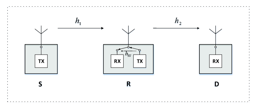
(a) The FD relay.

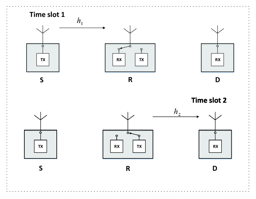
(b) The HD relay.

Figure 1: System model of X-duplex Relay.

II-A End-to-End SINR

In the FD mode, both RX and TX chains at node R are active at the same time. The signal received at node R is given as

$${y_{r}}={h_{1}}\sqrt{{P_{S}}}x+{h_{RI}}\sqrt{{P_{R}}}{x_{r}}+{n_{1}},$$ (1)

where ${h_{1}}$ denotes the channel between source and relay, $h_{RI}$ is the residual self interference of relay R. $x$ and ${x_{r}}$ denote the transmit signal of the source and relay. ${P_{S}}$ and ${P_{R}}$ are the transmit powers of the source and relay node. ${n_{1}}$ is the zero-mean-value additive white Gaussian noise with the power ${\sigma^{2}}$.

AF protocol is adopted at relay R and the forwarding signal at the relay R can be written as

$${x_{r}}={\beta_{f}}\cdot{y_{r}},$$ (2)

where ${\beta_{f}}$ denotes the power amplification factor satisfying

$$E[|{x_{r}}{|^{2}}]={\beta_{f}}^{2}(|{h_{1}}{|^{2}}{P_{S}}+|{h_{RI}}{|^{2}}{P_{R}}+{\sigma^{2}})\leq 1,$$ (3)

where

$${\beta_{f}}^{2}=\frac{1}{{|{h_{1}}{|^{2}}{P_{S}}+|{h_{RI}}{|^{2}}{P_{R}}+{\sigma^{2}}}}.$$ (4)

The received signal at the destination D is given by

$${y_{d}}={h_{2}}\sqrt{{P_{R}}}{x_{r}}+{n_{2}},$$ (5)

where ${h_{2}}$ denotes the channel between relay and destination, and ${n_{2}}$ is the zero-mean-value additive white Gaussian noise with power ${\sigma^{2}}$.

The end-to-end SINR of FD mode can be expressed as

$${\gamma_{F}}=\frac{{{P_{S}}{P_{R}}|{h_{1}}{|^{2}}|{h_{2}}{|^{2}}{\beta_{f}}^{2}}}{{{P_{R}}^{2}|{h_{2}}{|^{2}}|{h_{RI}}{|^{2}}{\beta_{f}}^{2}+{P_{R}}|{h_{2}}{|^{2}}{\beta_{f}}^{2}{\sigma^{2}}+{\sigma^{2}}}},$$ (6)

using (4) , the SINR can be further simplified as

$${\gamma_{F}}=\frac{{{P_{S}}{P_{R}}{\gamma_{1}}{\gamma_{2}}}}{{{P_{S}}{\gamma_{1}}+({P_{R}}{\gamma_{2}}+1)({P_{R}}{\gamma_{R}}+1)}}=\frac{{{X_{1}}{P_{R}}{\gamma_{2}}}}{{{X_{1}}+{P_{R}}{\gamma_{2}}+1}},$$ (7)

where ${\gamma_{1}}=\frac{{|{h_{1}}{|^{2}}}}{{{\sigma^{2}}}}$,${\gamma_{2}}=\frac{{|{h_{2}}{|^{2}}}}{{{\sigma^{2}}}}$,${\gamma_{R}}=\frac{{|{h_{RI}}{|^{2}}}}{{{\sigma^{2}}}}$ denote the respective channel SNRs and ${X_{1}}=\frac{{{P_{S}}{\gamma_{1}}}}{{{P_{R}}{\gamma_{R}}+1}}$.

In the HD mode, the relay R receives the signal from the source at the first half of a time slot, and it is given by

$${y_{r}}={h_{1}}\sqrt{{P_{S}}}x+{n_{1}},$$ (8)

At second half of a time slot, relay R transmits the received signal to the destination D with AF protocol. The received signal at destination D is given by

$${y_{d}} = {h_{2}}\sqrt{{P_{R}}}{x_{r}}+{n_{2}},$$ (9)

$${x_{r}} = {\beta_{h}}{y_{r}},$$ (10)

where ${\beta_{h}}$ is the amplification factor. Under transmit power constraint at relay R, ${\beta_{h}}$ can be expressed as

$${\beta_{h}}^{2}=\frac{1}{{|{h_{1}}{|^{2}}{P_{s}}+{\sigma^{2}}}}.$$ (11)

At destination D, the end-to-end SINR is thus given by

$${\gamma_{H}}{\rm{}}=\frac{{{P_{S}}{P_{R}}{\gamma_{1}}{\gamma_{2}}}}{{{P_{S}}{\gamma_{1}}+{P_{R}}{\gamma_{2}}+1}}.$$ (12)

The instantaneous SNRs ${\gamma_{1}}$ , ${\gamma_{2}}$ are modeled as the exponential random variable with respective means ${\lambda_{1}}$ and ${\lambda_{2}}$. In the X-duplex relay system, the self interference at relay is mitigated with effective self interference cancellation techniques [4, 5, 6, 7, 8, 9, 10, 11, 12, 13, 14]. The residual self interference at relay is assumed to follow the Rayleigh distribution[5]. At the relay R, the SNR of residual self interference ${\gamma_{R}}$ follows the exponential distribution with mean value ${\lambda_{R}}$. The residual self interference level is denoted as $\eta=\frac{{{\lambda_{R}}{P_{R}}}}{{{\lambda_{1}}{P_{S}}}}$. As the source signal might behave as interference to the self interference cancellation in active self interference cancellation schemes, the value of $\eta$ might vary with ${P_{S}}{\gamma_{1}}$. If only passive cancellation is applied, $\eta$ might be independent to ${P_{S}}{\gamma_{1}}$. In this paper, $\eta$ is merely used to denote the ratio of the average power of residual self interference ${\lambda_{R}}{P_{R}}$ and received signal at relay ${\lambda_{1}}{P_{S}}$, and is not assumed to be constant.

II-B X-duplex Relay

The HD mode outperforms the FD mode in the severe self interference region. To optimize the system performance, we consider a X-duplex relay which can be reduced to either FD or HD with different RF chain configurations based on the instantaneous SINR. The CSI of the self interference ${h_{RI}}$ can be measured by sufficient training [30][31]. The CSI of ${h_{1}}$ and ${h_{2}}$ can be obtained through pilot-based channel estimation. We also assume that reliable feedback channels are deployed, therefore the CSIs can be transmitted to the decision node.

The system’s average sum rate under FD and HD modes can be expressed as

$${R_{FD}}={\log_{2}}({\gamma_{F}}+1),{R_{HD}}={\log_{2}}(\sqrt{{\gamma_{H}+1}}),$$ (13)

where ${\gamma_{F}}$ , ${\gamma_{H}}$ denotes the SINR of the FD and HD modes, respectively.

To maximize the instantaneous sum rate, the instantaneous SINR of X-duplex relay can be given by

$${\gamma_{\max}}=\max\{{\gamma_{F}},\sqrt{{\gamma_{H}+1}}-1\}.$$ (14)

II-C Adaptive Power Allocation

In order to further optimise the system performance, we introduce the adaptive power allocation (PA) in the X-duplex relay to maximize the relay system’s end-to-end SINR subject to the total transmit power constraint, ${P_{S}}+{P_{R}}=P$. The optimal PA scheme for FD mode and HD mode based on the instantaneous CSIs is given by[21]

$${P_{S,FD\_PA}}=\frac{{\sqrt{P{\gamma_{1}}+1}}}{{\sqrt{P{\gamma_{1}}+1}+\sqrt{\left({P{\gamma_{2}}+1}\right)\left({P{\gamma_{R}}+1}\right)}}}P,{P_{S,HD\_PA}}=\frac{{\sqrt{P{\gamma_{1}}+1}}}{{\sqrt{P{\gamma_{1}}+1}+\sqrt{P{\gamma_{2}}+1}}}P,$$

$${P_{R,FD\_PA}}=\frac{{\sqrt{({P{\gamma_{2}}+1})({P{\gamma_{R}}+1})}}}{{\sqrt{P{\gamma_{1}}+1}+\sqrt{\left({P{\gamma_{2}}+1}\right)\left({P{\gamma_{R}}+1}\right)}}}P,{P_{R,HD\_PA}}=\frac{{\sqrt{P{\gamma_{2}}+1}}}{{\sqrt{P{\gamma_{1}}+1}+\sqrt{P{\gamma_{2}}+1}}}P.\vspace{-2mm}$$ (15)

Based on (II-C), the respective end-to-end SINR of FD and HD modes with PA are derived as

$${\gamma_{fd\_pa}}=\frac{{{P^{2}}{\gamma_{1}}{\gamma_{2}}}}{{P({\gamma_{1}}+{\gamma_{2}}+{\gamma_{R}})+2+2\sqrt{(P{\gamma_{1}}+1)(P{\gamma_{2}}+1)(P{\gamma_{R}}+1)}}},$$

$${\gamma_{hd\_pa}}=\frac{{{P^{2}}{\gamma_{1}}{\gamma_{2}}}}{{P({\gamma_{1}}+{\gamma_{2}})+2+2\sqrt{(P{\gamma_{1}}+1)(P{\gamma_{2}}+1)}}}.$$ (16)

Therefore, the instantaneous SINR of X-duplex relay with PA can be given by

$${\gamma_{xd\_pa}}=\max\{{\gamma_{fd\_pa}},\sqrt{{\gamma_{hd\_pa}}+1}-1\}.$$ (17)

III Performance Analysis

In this section, we present the CDF of the X-duplex relay and analyze the performance of the X-duplex system, including the outage probability, SER and the average sum rate. The derived expressions of performance of X-duplex with one shared antenna are essentially equivalent to the conventional system with two separated antennas [21].s

Lemma 1

The asymptotic complementary CDF of $\gamma_{F}$ is given by

$$\Pr({\gamma_{F}}>x)\approx\frac{{{\beta_{1}}}}{{1+\eta x}}{K_{1}}({\beta_{1}}){e^{-Cx}}-\frac{{2\eta({x^{2}}+x)}}{{\lambda_{2}}{P_{R}}{{{(1+\eta x)}^{2}}}}{K_{0}}({\beta_{1}}){e^{-Cx}},$$ (18)

where $C=\left({\frac{1}{{{\lambda_{1}}{P_{S}}}}+\frac{1}{{{\lambda_{2}}{P_{R}}}}}\right)$, ${\beta_{1}}=2\sqrt{\frac{{x+{x^{2}}}}{{{\lambda_{1}}{\lambda_{2}}{P_{S}}{P_{R}}}}}$, ${K_{1}}(\cdot)$ , ${K_{0}}(\cdot)$ are the first and zero order Bessel function of the second kind [37].

Proof:

The derivation is presented in Appendix A. ∎

Lemma 2

The complementary CDF of $\sqrt{{\gamma_{H}}+1}-1$ is given by

$$\Pr\left({{\gamma_{H}}>{x^{2}}+2x}\right)=\frac{1}{{{\lambda_{2}}}}\int\limits_{({x^{2}}+2x)/{P_{R}}}^{\infty}{{e^{-\frac{1}{{{P_{S}}{\lambda_{1}}}}({x^{2}}+2x+\frac{{{{({x^{2}}+2x)}^{2}}+{x^{2}}+2x}}{{{P_{R}}{\gamma_{2}}-{x^{2}}-2x}})-\frac{1}{{{\lambda_{2}}}}{\gamma_{2}}}}d{\gamma_{2}}}{\rm{=}}{\beta_{2}}{K_{1}}({\beta_{2}}){e^{-C({x^{2}}+2x)}},$$ (19)

where ${\beta_{2}}=2\sqrt{\frac{{{{({x^{2}}+2x)}^{2}}+{x^{2}}+2x}}{{{\lambda_{1}}{\lambda_{2}}{P_{S}}{P_{R}}}}}$ .

Proof:

The HD mode’s end-to-end SINR is given in (12), with the help of [38, eq.(3.324.1)], (19) can be obtained. ∎

Lemma 3

The asymptotic probability of $\{{\gamma_{F}}>x,{\gamma_{H}}>{x^{2}+2x}\}$ can be obtained as

$$\Pr({\gamma_{F}}>x,{\gamma_{H}}>{x^{2}+2x}){\rm{=}}{I_{1}}+{I_{2}},$$ (20)

where ${I_{1}}$, ${I_{2}}$ are expressed as

$${I_{1}} =\frac{{{\beta_{3}}}}{{1+\eta x}}{K_{1}}({\beta_{3}}){e^{-{\beta_{4}}}}-\frac{{2\eta({x^{2}}+x)}}{{{\lambda_{2}}{P_{R}}{{(1+\eta x)}^{2}}}}{K_{0}}({\beta_{3}}){e^{-{\beta_{4}}}},$$ (21)

$${I_{2}} ={\beta_{2}}{K_{1}}({\beta_{2}}){e^{-C(x^{2}+2x)}}-{\beta_{3}}{K_{1}}({\beta_{3}}){e^{-{\beta_{4}}}},$$ (22)

where ${\beta_{3}}=2\sqrt{\frac{{{{({x^{2}}+2x)}^{2}}+{x^{2}}+2x+\frac{1}{\eta}(x+1)({x^{2}}+2x)}}{{{\lambda_{1}}{\lambda_{2}}{P_{S}}{P_{R}}}}}$ , ${\beta_{4}}=C({x^{2}}+2x)+\frac{{x+1}}{{\eta{\lambda_{1}}{P_{S}}}}$.

Proof:

The derivation is presented in Appendix B. ∎

III-A Distribution of the Received Signal

Proposition 1

The asymptotic CDF of X-duplex relay system’s SINR ${\gamma_{\max}}$ can be derived as

$$\Pr({\gamma_{\max}}<x) =1-\frac{1}{{1+\eta x}}\left[{{\beta_{1}}{K_{1}}({\beta_{1}}){e^{-Cx}}+\eta x{\beta_{3}}{K_{1}}({\beta_{3}}){e^{-{\beta_{4}}}}}\right]$$ (23)

$$+\frac{{2\eta({x^{2}}+x)}}{{{\lambda_{2}}{P_{R}}{{(1+\eta x)}^{2}}}}\left[{{K_{0}}({\beta_{1}}){e^{-Cx}}-{K_{0}}({\beta_{3}}){e^{-{\beta_{4}}}}}\right],\vspace{-2mm}$$

where $\eta=\frac{{{\lambda_{R}}{P_{R}}}}{{{\lambda_{1}}{P_{S}}}}$, $C={\frac{1}{{{\lambda_{1}}{P_{S}}}}+\frac{1}{{{\lambda_{2}}{P_{R}}}}}$, ${\beta_{1}}=2\sqrt{\frac{{x+{x^{2}}}}{{{\lambda_{1}}{\lambda_{2}}{P_{S}}{P_{R}}}}}$, ${\beta_{2}}=2\sqrt{\frac{{{{({x^{2}}+2x)}^{2}}+{x^{2}}+2x}}{{{\lambda_{1}}{\lambda_{2}}{P_{S}}{P_{R}}}}}$ , ${\beta_{3}}=2\sqrt{\frac{{{{({x^{2}}+2x)}^{2}}+{x^{2}}+2x+\frac{1}{\eta}(x+1)({x^{2}}+2x)}}{{{\lambda_{1}}{\lambda_{2}}{P_{S}}{P_{R}}}}}$ , ${\beta_{4}}=C({x^{2}}+2x)+\frac{{x+1}}{{\eta{\lambda_{1}}{P_{S}}}}$, ${K_{1}}(\cdot)$, ${K_{0}}(\cdot)$ are the first and zero order Bessel function of the second kind.

Proof:

According to the permutation theorem, the CDF expression can be obtained as

$$\Pr({\gamma_{\max}}<x) =\Pr({\gamma_{F}}<x,\sqrt{{\gamma_{H}+1}}-1<x)$$ (24)

$$=1-\Pr({\gamma_{F}}>x)-\Pr({\gamma_{H}}>{x^{2}+2x})+\Pr({\gamma_{F}}>x,{\gamma_{H}}>{x^{2}+2x}).$$

With the help of Lemma 1, Lemma 2, Lemma 3, (23) is derived. ∎

III-B Outage Probability

The outage probability can be given as

$${P_{*}}=\Pr({\log_{2}}(1+SINR)<{R_{0}})={F_{{\gamma}}}(T),$$ (25)

where the threshold of the outage probability is set to ensure the transmit rate over $R_{0}$ bps/Hz, $T={2^{{R_{0}}}}-1$ and ${F_{\gamma}}(\cdot)$ is CDF of the end-to-end SINR $\gamma$.

The X-duplex relay configures the antenna to provide the maximum sum rate of the relay network. With the CDF expression in (23) and (25), the outage probability of the X-duplex relay system can be derived.

From Lemma 1 and (25), the outage probability of the FD mode can be obtained. According to [39, eq.(10.30)], in the high SNR condition, when $z$ comes close to zero, the ${K_{1}}(z)$ function converges to $\frac{1}{z}$, and the value of ${K_{0}}(z)$ is comparatively small. Therefore, in the high SNR scenarios, the FD mode’s outage probability is approximately given by

$${P_{out\_FD}}(x)\approx 1-\frac{1}{{1+\eta x}}{e^{-Cx}},$$ (26)

when the SNR goes infinite, the outage probability of FD mode will approach

$$P_{out\_FD}^{\infty}(x)=\frac{{\eta x}}{{1+\eta x}}.$$ (27)

Therefore, the outage probability of FD mode is limited by the error floor which is caused by self interference at high SNR.

By substituting (23) into (25), the outage probability of X-duplex relay system can be obtained. In the high SNR, the outage probability can be derived using the similar approximation in (26),

$$P_{out\_XD}^{\infty}(x)\approx 1-\frac{1}{{1+\eta x}}{e^{-Cx}}-\frac{{\eta x}}{{1+\eta x}}{e^{-{\beta_{4}}}},$$ (28)

when the SNR goes infinite, the outage probability of X-duplex relay system approaches to zero, indicating that there is no performance floor for X-duplex relay system in the high SNR region.

For the X-duplex relay system, the finite diversity order of SNR is provided by [32]

$$d(\lambda)=-\frac{{\partial\ln{P_{out}}(\lambda)}}{{\partial\ln\lambda}}=-\frac{\lambda}{{{P_{out}}(\lambda)}}\frac{{\partial{P_{out}}(\lambda)}}{{\partial\lambda}},$$ (29)

where ${{P_{out}}(\lambda)}$ is the system’s outage probability at average SNR ${\lambda}$. We use this equation to calculate the diversity order of X-duplex relay system.

We assume the transmit power of the source and relay is the same under fixed power allocation condition, $P_{S}=P_{R}=P_{t}$. The diversity order ${d_{XD}}$ of the X-duplex relay system is given as

$${d_{XD}}=\frac{1}{{{P_{t}}}}\frac{{\frac{x}{{1+\eta x}}(\frac{1}{{{\lambda_{1}}}}+\frac{1}{{{\lambda_{2}}}}){e^{-Cx}}+\frac{{\eta x}}{{1+\eta x}}\left[{(\frac{1}{{{\lambda_{1}}}}+\frac{1}{{{\lambda_{2}}}})({x^{2}}+2x)+\frac{{x+1}}{{\eta{\lambda_{1}}}}}\right]{e^{-{\beta_{4}}}}}}{{1-\frac{1}{{1+\eta x}}{e^{-Cx}}-\frac{{\eta x}}{{1+\eta x}}{e^{-{\beta_{4}}}}}}.$$ (30)

Furthermore, the diversity order ${d_{XD}}$ can be estimated by using the Taylor’s formula in [38, eq.(1.211)] in the high transmit power scenario

$${d_{XD}}\approx\frac{{{C_{1}}x+\eta x{C_{1}}({x^{2}}+2x)+\eta x\frac{{x+1}}{{\eta{\lambda_{1}}}}-\frac{1}{{{P_{t}}}}\left[{{{({C_{1}}x)}^{2}}+\eta x{{\left({{C_{1}}({x^{2}}+2x)+\frac{{x+1}}{{\eta{\lambda_{1}}}}}\right)}^{2}}}\right]}}{{{C_{1}}x+\eta x{C_{1}}({x^{2}}+2x)+\eta x\frac{{x+1}}{{\eta{\lambda_{1}}}}}},$$ (31)

where ${C_{1}}=\frac{1}{{{\lambda_{1}}}}+\frac{1}{{{\lambda_{2}}}}$. When the transmit power goes infinite, the diversity order of X-duplex relay system approaches to one, indicating that there is no error floor in the system.

For the HD mode, from equation (13), the HD mode’s equivalent SINR in one time slot is given as $\sqrt{{\gamma_{H}}+1}-1$. Therefore, the outage probability of HD mode can be obtained with (19)

$${P_{out\_HD}}(x)=1-{\beta_{2}}{K_{1}}({\beta_{2}}){e^{-C({x^{2}}+2x)}}\approx 1-{e^{-C(x^{2}+2x)}}.$$ (32)

The finite-SNR diversity orders of FD and HD mode can be written as

$${d_{FD}} = \frac{1}{{{P_{t}}}}\frac{{(\frac{1}{{{\lambda_{1}}}}+\frac{1}{{{\lambda_{2}}}})\frac{x}{{1+\eta x}}{e^{-Cx}}}}{{1-\frac{1}{{1+\eta x}}{e^{-Cx}}}}\approx\frac{{1-\frac{x}{{{P_{t}}}}(\frac{1}{{{\lambda_{1}}}}+\frac{1}{{{\lambda_{2}}}})}}{{1+{P_{t}}\eta\frac{{{\lambda_{1}}{\lambda_{2}}}}{{{\lambda_{1}}+{\lambda_{2}}}}}},$$

$${d_{HD}} = \frac{1}{{{P_{t}}}}\frac{{(\frac{1}{{{\lambda_{1}}}}+\frac{1}{{{\lambda_{2}}}})({x^{2}}+2x)\cdot{e^{-C({x^{2}}+2x)}}}}{{1-{e^{-C({x^{2}}+2x)}}}}\approx 1-\frac{1}{{{P_{t}}}}(\frac{1}{{{\lambda_{1}}}}+\frac{1}{{{\lambda_{2}}}})({x^{2}}+2x),$$ (33)

At medium SNR and low residual self interference, the diversity order of FD can be approximated as ${d_{FD}}\approx{1-\frac{x}{{{P_{t}}}}(\frac{1}{{{\lambda_{1}}}}+\frac{1}{{{\lambda_{2}}}})}$. With optimal self interference cancellation, $d_{FD}$ approaches one in high SNR region. When the SNR goes infinite, the diversity order of the FD and HD mode approaches to zero and one respectively, indicating that the outage probability curve of X-duplex relay system is parallel with HD mode when SNR reaches this region.

The outage probability intersection of FD and HD mode can be calculated as

$${P_{t}}^{*}=({\frac{1}{{{\lambda_{1}}}}+\frac{1}{{{\lambda_{2}}}}})\frac{{{x^{2}}+x}}{{\ln(1+\eta x)}},$$ (34)

when $P_{t}<P_{t}^{*}$, the outage probability of FD is lower than HD. The intersection point is affected by self interference level $\eta$. When $\eta$ reaches zero, the intersection point goes infinite, indicating that FD outperforms HD in all SNR circumstances with ideal self interference cancellation.

III-C Average SER Analysis

For linear modulation formats, the average SER can be computed as [36]

$$\overline{SER}={a_{1}}{\mathbb{E}}[Q(\sqrt{2{a_{2}}\gamma})]=\frac{{{a_{1}}\sqrt{{a_{2}}}}}{{2\sqrt{\pi}}}\int\limits_{0}^{\infty}{\frac{{{e^{-{a_{2}}\gamma}}}}{{\sqrt{\gamma}}}{F_{\gamma}}(\gamma)d\gamma},$$ (35)

where ${F_{\gamma}}(\cdot)$ is the CDF of $\gamma$, and $Q(\cdot)$ is the Gaussian Q-Function [38]. The parameters $({a_{1}},{a_{2}})$ denote the modulation formats, e.g., ${a_{1}}=1,{a_{2}}=1$ for the binary phase-shift keying (BPSK) modulation [36, eq.(6.6)].

Proposition 2

The asymptotic average SER of the X-duplex relay system can be derived as

$$\overline{SER}\approx\frac{{{a_{\rm{1}}}\sqrt{{a_{2}}}}}{{2\sqrt{\pi}}}\left\{{{a_{2}}^{-\frac{1}{2}}\Gamma(\frac{1}{2})-\frac{1}{{\sqrt{\eta}}}{e^{\frac{1}{\eta}({a_{2}}+C)}}\Gamma(\frac{1}{2})\Gamma(\frac{1}{2},\frac{1}{\eta}({a_{2}}+C))}\right.$$ (36)

$$-\eta{e^{-\frac{1}{{{\lambda_{1}}{P_{S}}\eta}}}}{\left({2C}\right)^{-\frac{3}{4}}}\Gamma(\frac{3}{2})\exp(\frac{{{\mu_{1}}^{2}}}{{8C}}){D_{-\frac{3}{2}}}(\frac{{{\mu_{1}}}}{{\sqrt{2C}}})\left.{-\frac{1}{2}{\eta^{3}}{e^{-\frac{1}{{{\lambda_{1}}{P_{S}}\eta}}}}{{\left({2C}\right)}^{-\frac{7}{4}}}\Gamma(\frac{7}{2})\exp(\frac{{{\mu_{2}}^{2}}}{{8C}}){D_{-\frac{7}{2}}}(\frac{{{\mu_{2}}}}{{\sqrt{2C}}})}\right\},$$

where ${\mu_{1}}={a_{2}}+2C+\frac{1}{{{\lambda_{1}}{P_{S}}\eta}}+\eta$, ${\mu_{2}}={a_{2}}+2C+\frac{1}{{{\lambda_{1}}{P_{S}}\eta}}+\frac{5}{3}\eta$, $\Gamma(\cdot)$ is the Gamma Function, $\Gamma(a,x)$ is the incomplete Gamma Function, ${D_{p}}(\cdot)$ is the Parabolic Cylinder Function [38].

Proof:

The derivation is presented in Appendix C. ∎

According to (23), when SNR goes infinite, the CDF of $\gamma_{\max}$ becomes $\Pr({\gamma_{\max}}<x)=0$, the SER of X-duplex relay system comes to zero.

For the FD mode and HD mode, the average SER can be given as

$${\overline{SER}_{FD}} \approx\frac{{{a_{\rm{1}}}\sqrt{{a_{2}}}}}{{2\sqrt{\pi}}}\left\{{{a_{2}}^{-\frac{1}{2}}\Gamma(\frac{1}{2})-\frac{1}{{\sqrt{\eta}}}{e^{\frac{1}{\eta}({a_{2}}+C)}}\Gamma(\frac{1}{2})\Gamma(\frac{1}{2},\frac{1}{\eta}({a_{2}}+C))}\right\},$$

$${\overline{SER}_{HD}} \approx\frac{{{a_{\rm{1}}}\sqrt{{a_{2}}}}}{{2\sqrt{\pi}}}\left\{{{a_{2}}^{-\frac{1}{2}}\Gamma(\frac{1}{2})-{{(2C)}^{-\frac{1}{2}}}\Gamma(\frac{1}{2})exp(\frac{{{{({a_{2}}+2C)}^{2}}}}{{8C}}){D_{-\frac{1}{2}}}(\frac{{{a_{2}}+2C}}{{\sqrt{2C}}})}\right\}.$$ (37)

For the FD mode, when SNR goes infinite, the CDF of FD mode approaches $\Pr({\gamma_{FD}}<x)=1-\frac{1}{{1+\eta x}}$. With (35) and [38, eq.(3.383.10)], the SER of FD mode can be obtained.

$${\overline{SER}_{FD\_SNR\to\infty}}=\frac{{{a_{1}}\sqrt{{a_{2}}}}}{{2\sqrt{\pi}}}\int\limits_{0}^{\infty}{\frac{{{e^{-{a_{2}}x}}}}{{\sqrt{x}}}(1-\frac{1}{{1+\eta x}})dx}=\frac{{{a_{1}}\sqrt{{a_{2}}}}}{{2\sqrt{\pi}}}{\left({\frac{1}{\eta}}\right)^{1/2}}{e^{\frac{1}{\eta}{a_{2}}}}\Gamma(\frac{3}{2})\Gamma(-\frac{1}{2},\frac{1}{\eta}{a_{2}}).\\$$

From (III-C), it can be seen that the SER of FD mode is restricted by the lower bound, determined by self interference level $\eta$, $a_{1}$, $a_{2}$. Compared with FD mode, the X-duplex relay system removes the error floor and achieves lower SER in high SNR region.

III-D Average Sum Rate

By using the CDF of ${\gamma_{\max}}$, the average sum rate of X-duplex system is derived in this section.

$$\bar{R}={\mathbb{E}}[{\log_{2}}(1+\gamma)]=\frac{1}{{\ln 2}}\int\limits_{0}^{\infty}{\frac{{1-{F_{\gamma}}(x)}}{{1+x}}}dx,$$ (38)

where ${F_{\gamma}}(\cdot)$ is the CDF of $\gamma$.

In order to simplify the final average sum rate expression, ${w_{i1}}(a,b)$ and ${w_{i2}}$ are introduced to denote the approximate value of integral $\int_{b}^{\infty}{{e^{-C{x^{2}}}}/(x+a)dx}$ and $\int_{1+\frac{1}{{4\eta}}}^{1+\frac{5}{{4\eta}}}{{e^{-C{x^{2}}}}/(x+\frac{3}{{4\eta}})dx}$, given in Lemma 4 and 5.

Lemma 4

when $\left|b\right|>\left|a\right|>0$, the exact value of integral ${w_{i1}}(a,b)=\int_{b}^{\infty}{{e^{-C{x^{2}}}}/(x+a)dx}$ is given by

$${w_{i1}}(a,b)=\frac{1}{{2a}}\sqrt{\frac{\pi}{C}}\left[{1-\Phi(C{b^{2}})}\right]+\frac{{{e^{-C{a^{2}}}}}}{2}{E_{1}}(C({b^{2}}-{a^{2}}))-\frac{{{e^{-\frac{{C{b^{2}}}}{2}}}}}{{2a}}\sum\limits_{k=1}^{\infty}{{a^{2k-2}}{C^{k-\frac{3}{2}}}{{(C{b^{2}})}^{\frac{1}{4}-\frac{k}{2}}}{W_{\frac{1}{4}-\frac{k}{2},\frac{3}{4}-\frac{k}{2}}}(C{b^{2}})},$$ (39)

where $\Phi(\cdot)$ is the probability integral, and ${W_{\lambda,\mu}}(z)$ is the Whittaker function [38], we use the first ${{N}}$ items of the third part of (39) for approximation, denoted as ${w_{i1}}(a,b,N)$.

Proof:

The derivation is presented in Appendix D. ∎

Lemma 5

The approximate value of integral ${w_{i2}}=\int_{\rho}^{1+\frac{1}{\eta}}{{e^{-C{x^{2}}}}/(x+\frac{1}{\eta}-\rho)dx}$ is given by

$${w_{i2}}\approx{e^{-C{\rho^{2}}+2C\rho\frac{1}{\eta}}}\sum\limits_{k=0}^{{N_{2}}}{\frac{{{{(-C)}^{k}}}}{{k!{\eta^{2k}}}}\left[{{E_{1}}({\varepsilon_{1}})-{E_{1}}({\varepsilon_{2}})}\right]}+{e^{-C{\rho^{2}}+2C\rho\frac{1}{\eta}}}\sum\limits_{k=1}^{{N_{2}}}{\sum\limits_{l=1}^{2k}{\frac{{{{(-C)}^{k}}}}{{k!{{(2C\rho)}^{l}}{{(-\eta)}^{2k-l}}}}(\begin{array}[]{*{20}{c}}{2k}\\ l\end{array})}}\left[{\gamma(l,{\varepsilon_{2}})-\gamma(l,{\varepsilon_{1}})}\right],$$ (40)

where ${\varepsilon_{0}}=1+\frac{2}{\eta}-\rho$, ${\varepsilon_{1}}=2C\rho\frac{1}{\eta}$, ${\varepsilon_{2}}=2C\rho{\varepsilon_{0}}$, $\gamma(a,x)$ is the incomplete Gamma Function, first ${{N_{2}}}$ items are used to approximate value.

Proof:

The derivation is presented in Appendix E. ∎

Proposition 3

The average sum rate of X-duplex system can be expressed approximately as

$$\bar{R}\approx \frac{1}{{\ln 2}}\left\{\frac{{\rm{1}}}{{1-\eta}}\left[{{e^{C}}{E_{1}}(C)-{e^{\frac{C}{\eta}}}{E_{1}}(\frac{C}{\eta})}\right]-\frac{2}{{{\lambda_{2}}{P_{R}}{C_{2}}}}{e^{\frac{C}{{2\eta}}}}{\Gamma^{2}}(2){W_{-\frac{3}{2},0}}({z_{1}}){W_{-\frac{3}{2},0}}({z_{2}})\right.$$ (41)

$$\left.{+\frac{\eta}{{\eta-1}}{e^{C{\rho^{2}}-\frac{1}{{{\lambda_{1}}{P_{S}}\eta}}}}\left[{{w_{i1}}(1-\rho,\rho,{N_{1}})-\frac{1}{\eta}{w_{i1}}(\frac{1}{\eta}-\rho,1+\frac{1}{\eta},{N_{3}})-\frac{1}{\eta}{w_{i2}}}\right]}\right\}.$$

where ${C_{2}}=\frac{2}{{\sqrt{{\lambda_{1}}{\lambda_{2}}{P_{S}}{P_{R}}}}}$, ${z_{1}}=\frac{{C+\sqrt{{C^{2}}-{{C_{2}}^{2}}}}}{{2\eta}}$, ${z_{2}}=\frac{{C-\sqrt{{C^{2}}-{{C_{2}}^{2}}}}}{{2\eta}}$, ${W_{\lambda,\mu}}(z)$ is the Whittaker functions [38].

Proof:

The derivation is presented in Appendix F. ∎

According to (23) and (38), when SNR goes infinite, the CDF of $\gamma_{\max}$ becomes $\Pr({\gamma_{\max}}<x)=1-H(x-1)-H(1-x)=0$ and the average sum rate of X-duplex relay system can be derived as,

$${{\bar{R}}_{XD\_SNR\to\infty}}=\frac{1}{{\ln 2}}\int\limits_{0}^{\infty}{\frac{1}{{1+x}}}dx.$$ (42)

It can be observed that the maximal achievable average sum rate of X-duplex relay system is not restricted by the self interference.

The approximate average sum rate of FD mode and HD mode can be given as

$${{\bar{R}}_{FD}}\approx\frac{1}{{\ln 2}}\frac{{\rm{1}}}{{1-\eta}}\left[{{e^{C}}{E_{1}}(C)-{e^{\frac{C}{\eta}}}{E_{1}}(\frac{C}{\eta})}\right],{{\bar{R}}_{HD}}\approx\frac{1}{{2\ln 2}}{e^{C}}{E_{1}}(C),$$ (43)

When SNR goes infinite, the upper bound of FD mode can be derived [38, eq.(3.195)].

$${{\bar{R}}_{FD\_SNR\to\infty}}=\frac{1}{{\ln 2}}\int\limits_{0}^{\infty}{\frac{1}{{1+x}}\frac{1}{{1+\eta x}}}dx=\frac{{\ln\eta}}{{(\eta-1)\ln 2}}.$$ (44)

The upper bound of the average sum rate of FD mode is given in (44). It means that the practical average sum rate cannot be larger than (44), which presents the achievable region of average sum rate of FD mode.

Comparing the (42) and (44), the X-duplex relay system overcomes the restriction of self interference compared with FD mode.

III-E Diversity order of XD-PA

In this subsection, a lower bound and a upper bound for the X-duplex relay’s end-to-end SINR with PA are provided and the CDF of these bounds are obtained. Finally, the diversity order of XD-PA is derived.

The lower bound and upper bound for the end-to-end SINR (17) can be written as

$$\mathcal{D}({\gamma_{lower}},{\gamma_{R}})\geq{\gamma_{xd\_pa}}\geq\mathcal{D}({\gamma_{upper}},{\gamma_{R}}),$$ (45)

where ${\gamma_{upper}}=\min\{{\gamma_{1}},{\gamma_{\rm{2}}}\}$, ${\gamma_{lower}}=\max{\rm{\{}}{\gamma_{\rm{1}}},{\gamma_{\rm{2}}}{\rm{\}}}$, $\mathcal{D}(x,y)=\max\{\mathcal{C}(x,y),{\sqrt{\mathcal{C}(x,0)+1}-1}\}$, $\mathcal{C}(x,y)=\frac{{{x^{2}}{P^{2}}}}{{2xP+yP+2+2(xp+1)\sqrt{yp+1}}}$. When $x\in(0,+\infty)$, the function $\mathcal{C}(x,y)$ is a monotonically increasing function. Therefore, the function $\mathcal{D}(x,y)$ is also monotonic when $x\in(0,+\infty)$.

The CDF distribution of ${\gamma_{upper}}$ , ${\gamma_{lower}}$ is given as

$${F_{{}_{{\gamma_{u}}}}}(x)=1-{e^{-\frac{1}{{{\lambda_{1}}}}x-\frac{1}{{{\lambda_{2}}}}x}},{F_{{}_{{\gamma_{l}}}}}(x)=(1-{e^{-\frac{1}{{{\lambda_{1}}}}x}})(1-{e^{-\frac{1}{{{\lambda_{2}}}}x}}).$$ (46)

With [38, eq.(3.322)], we can obtain the outage probability of the upper bound $\mathcal{D}({\gamma_{upper}},{\gamma_{R}})$

$${P_{{\gamma_{upper}}}}(x) =\Pr\{\mathcal{C}({\gamma_{u}},{\gamma_{R}})<x,\mathcal{C}({\gamma_{u}},0)<{x^{2}+2x}\}=\int_{0}^{\frac{2}{T}}{{f_{{\gamma_{u}}}}(t)dt}+\int_{\frac{2}{T}}^{{T_{2}}}{{e^{-\frac{{{T^{2}}{t^{2}}-2Tt}}{{P{\lambda_{R}}}}}}{f_{{\gamma_{u}}}}(t)dt}$$ (47)

$$={F_{{\gamma_{u}}}}(\frac{2}{T})+(\frac{1}{{{\lambda_{1}}}}+\frac{1}{{{\lambda_{2}}}})G(\frac{2}{T},{T_{2}},\frac{{P{\lambda_{R}}}}{{4{T^{2}}}},\frac{1}{{{\lambda_{1}}}}+\frac{1}{{{\lambda_{2}}}}-\frac{{2T}}{{P{\lambda_{R}}}}),$$

where $T=\frac{{\sqrt{x+1}-\sqrt{x}}}{{\sqrt{x}}}P$ , ${T_{2}}=\frac{{2({x^{2}}+2x)+2\sqrt{{{({x^{2}}+2x)}^{2}}+{x^{2}}+2x}}}{P}$, ${f_{{\gamma_{u}}}}(t)$ is the PDF of ${\gamma_{upper}}$, $G({u_{1}},{u_{2}},\beta,\gamma)=\sqrt{\pi\beta}{e^{\beta{\gamma^{2}}}}\left[{\Phi(\gamma\sqrt{\beta}+\frac{{{u_{2}}}}{{2\sqrt{\beta}}})-\Phi(\gamma\sqrt{\beta}+\frac{{{u_{1}}}}{{2\sqrt{\beta}}})}\right]$.

The Taylor expansion of the upper bound ${P_{{\gamma_{upper}}}}(x)$ is

$${P_{{\gamma_{upper}}}}(x){\rm{=}}\frac{{2({\lambda_{1}}{\rm{+}}{\lambda_{2}})}}{{{\lambda_{1}}{\lambda_{2}}}}\frac{{{x^{2}}+2x+\sqrt{{{({x^{2}}+2x)}^{2}}+{x^{2}}+2x}-\sqrt{{x^{2}}+x}-x}}{P}+o({P^{-\frac{3}{2}}}).$$ (48)

It can be observed that the diversity order of XD-PA is at least one.

Similarly, the outage probability of the lower bound $\mathcal{D}({\gamma_{upper}},{\gamma_{R}})$ can be calculated as

$${P_{{\gamma_{lower}}}}(x)= {F_{{\gamma_{l}}}}(\frac{2}{T})+\frac{1}{{{\lambda_{1}}}}G(\frac{2}{T},{T_{2}},\frac{{P{\lambda_{R}}}}{{4{T^{2}}}},\frac{1}{{{\lambda_{1}}}}-\frac{{2T}}{{P{\lambda_{R}}}})+\frac{1}{{{\lambda_{2}}}}G(\frac{2}{T},{T_{2}},\frac{{P{\lambda_{R}}}}{{4{T^{2}}}},\frac{1}{{{\lambda_{2}}}}-\frac{{2T}}{{P{\lambda_{R}}}})$$ (49)

$$-(\frac{1}{{{\lambda_{1}}}}+\frac{1}{{{\lambda_{2}}}})G(\frac{2}{T},{T_{2}},\frac{{P{\lambda_{R}}}}{{4{T^{2}}}},\frac{1}{{{\lambda_{1}}}}+\frac{1}{{{\lambda_{2}}}}-\frac{{2T}}{{P{\lambda_{R}}}}),$$

using Taylor’s formula, we can obtain

$${P_{{\gamma_{lower}}}}(x)=\frac{{2{\lambda_{R}}}}{{{\lambda_{1}}{\lambda_{2}}}}\frac{{{T_{3}}}}{{{P^{2}}}}\left({3\frac{{{\lambda_{1}}{\rm{+}}{\lambda_{2}}}}{{{\lambda_{1}}{\lambda_{2}}}}-\frac{8}{{{\lambda_{R}}}}\frac{{\sqrt{x+1}-\sqrt{x}}}{{\sqrt{x}}}}\right)+o({P^{-\frac{5}{2}}}),$$ (50)

where ${T_{3}}={(\sqrt{{x^{2}}+x}+x)^{2}}({x^{2}}+2x+\sqrt{{{({x^{2}}+2x)}^{2}}+{x^{2}}+2x}-\sqrt{{x^{2}}+x}-x)$.

It can be observed that the diversity order of XD-PA is at most two.

Similarly, the Taylor expansion of the upper bound and lower bound of the outage probability of the FD mode with PA can be provided as

$$P_{{\gamma_{upper}}}^{FD}(x) =\frac{{({\lambda_{1}}{\rm{+}}{\lambda_{2}})\sqrt{{\lambda_{R}}\pi}}}{{2{\lambda_{1}}{\lambda_{2}}}}\frac{{\sqrt{{x^{2}}+x}+x}}{{\sqrt{P}}}+o({P^{-1}}),$$

$$P_{{\gamma_{lower}}}^{FD}(x) =\frac{{{\lambda_{R}}}}{{{\lambda_{1}}{\lambda_{2}}}}\frac{{{{(\sqrt{{x^{2}}+x}+x)}^{2}}}}{P}+o({P^{-2}}),$$ (51)

The diversity order of FD with PA is between $\frac{1}{2}$ and $1$. As the diversity order of X-duplex is one at high SNR, the diversity order of X-duplex is higher than FD with PA at high SNR.

IV Simulation Results

In this section, simulations are provided to validate the performance analysis of the relay system with X-duplex relay. Without loss of generality, we set the SNRs of source-relay and relay-destination channel as one, $\lambda_{1}={\lambda_{2}}=1$. The transmit power of the source and relay is set as equal under the fixed power allocation condition, $P_{S}=P_{R}$. The threshold of the outage probability is set as 2 bps/Hz [19, 20]. It is shown in [8, 25, 33] that the self interference can be cancelled up to 110 dB. We assume the self interference cancellation ability is between 70dB and 110dB [34]. The path loss between source and relay is modeled as $P{L_{LOS}}\left(R\right)=103.4+24.2lo{g_{10}}\left(R\right)$ [35]. Therefore, the residual self interference level $\eta$ is set as ${\eta=0.2,0.05,0.01}$.

Fig. 2 demonstrates the outage probability performance of X-duplex relay system with different self interference $\eta=$ 0.2, 0.05 and 0.01. The outage performance of FD mode and HD mode is also illustrated for comparison. As can be seen, the exact outage probability curves tightly matches with the analytic expression given in (25). The figure reveals that X-duplex relay system’s outage probability is lower than both FD and HD schemes. At high SNR, the FD scheme has an error floor, which coincides with the analytical results in (27). When the SNR goes infinite, the X-duplex relay eliminates the error floor and remains the full diversity order, as shown in (31) and (III-B). The effect of self interference on the X-duplex relay system is very small at high SNR. This is because the HD mode is more likely to be selected in the X-duplex relay as the performance of FD mode is interference limited at high SNR. The X-duplex benefits more from the HD mode, whose performance is independent of residual self interference and improves with the increase of transmit power. Therefore, the impact of residual self interference from FD mode on X-duplex becomes smaller as SNR increases and the curves of X-duplex under different $\eta$ become close.

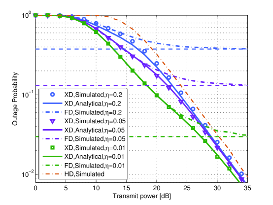
Figure 2: Outage probability of X-duplex relay system when $\eta{\rm{=0}}{\rm{.2}}$, 0.05, 0.01, the dashed lines of performance floor coincide with analytical results in (27), and the intersection point of FD and HD mode coincides with analytical results in (34).

Fig. 3 compares the finite SNR diversity order of X-duplex relay with pure FD and HD mode at $\eta=0.2,0.05,0.01$. The diversity order of X-duplex relay system increases with that of FD mode from low to medium SNR as FD mode is more likely to be selected in this region. When the diversity order of FD mode decreases, the performance of X-duplex relay system is influenced. As the performance of HD mode improves with SNR, the diversity order of X-duplex relay system increases as HD mode is more likely to be selected. When SNR goes infinity, the diversity order curve of X-duplex relay system approaches that of HD mode because FD mode encounters the performance floor. At high SNR, the X-duplex relay eliminates the error floor and achieves the full diversity order as the HD mode, which is consistent with Section III B.

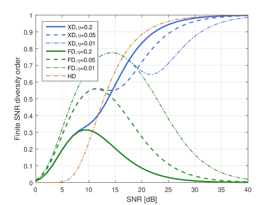
Figure 3: Finite SNR diversity order of FD mode, HD mode and X-duplex relay versus link SNR.

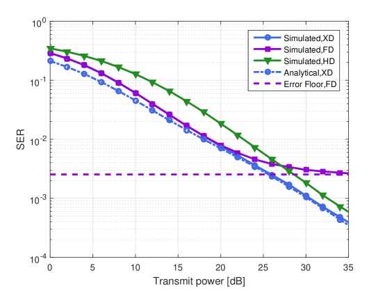
Figure 4: Average SER of X-duplex relay system when $\eta{\rm{=0}}{\rm{.01}}$, the dashed lines coincide with analytical results in (III-C).

Fig. 4 plots both the analytical and simulated results of the SER in the X-duplex relay system with $\eta{\rm{=0}}{\rm{.01}}$. The SER performance of FD and HD is depicted for comparison. From the figure, we can observe that X-duplex relay system achieves a better performance compared with pure FD and HD schemes. At high SNR , the X-duplex relay removes the performance floor. The curves of X-duplex and HD mode become close at high SNR as the benefit from FD mode is limited by the residual self interference.

Fig. 5 depicts the average sum rate of the X-duplex system versus SNR with $\eta=0.2$. The approximate analytical expression in (41) tightly approaches the exact average sum rate. It can be seen from the figure that X-duplex relay system provides a higher sum rate than that of FD and HD. The performance improvement of X-duplex is most significant at medium SNR.

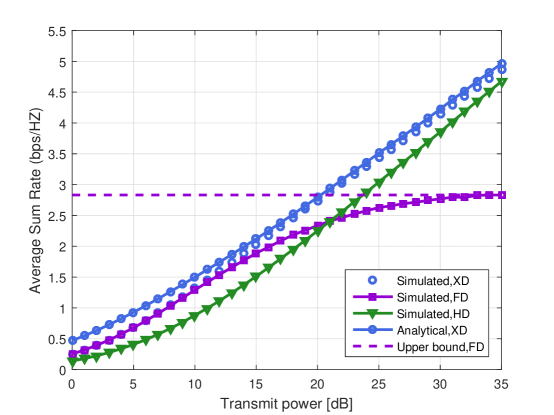
Figure 5: Average sum rate of X-duplex relay system when $\eta=0.2$, the dashed lines coincide with analytical results in (44).

In Fig. 6, the simulated average sum rate of the X-duplex system versus self interference with different levels of transmit power is depicted. In the weak self interference region, FD achieves a higher sum rate than HD. As self interference increases, the average sum rate of FD mode significantly decreases and performs worse than the HD mode. The average sum rate of X-duplex relay system is always better than FD and HD mode. The performance of X-duplex decreases quickly with the self interference increases, and is most obvious at high SNR. When the self interference is perfectly cancelled, the average sum rate of X-duplex is twice that of HD mode.

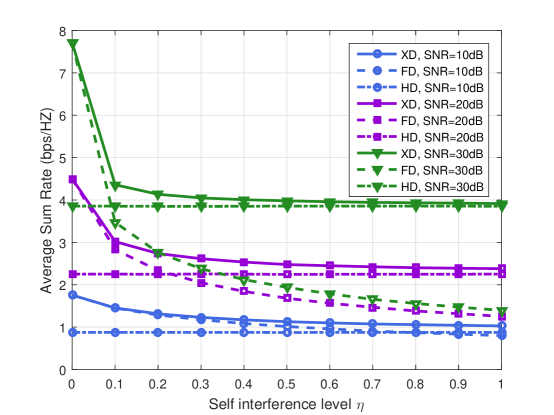
Figure 6: Average sum rate of X-duplex relay system versus self interference.

Fig. 7 illustrates the outage probability of XD-PA subject to the total power constraint. The performance of the X-duplex relay system with uniform power allocation, is illustrated for comparison. According to this figure, the outage probability performance of X-duplex relay system can be improved with adaptive power allocation compared with equal power allocation. The diversity order of XD-PA is between one and two. The performance of FD with power allocation is also plotted for comparison and the diversity order of FD-PA is between $\frac{1}{2}$ and one. It can observed that the diversity order of X-duplex is higher than FD with PA at high SNR, which coincide with the analysis in Section III E.

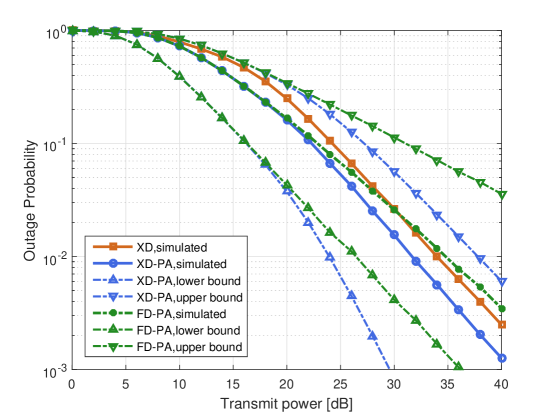
Figure 7: Outage probability of XD-PA versus the transmit power when $\eta=0.2$.

IV-A Differences and Discussions

The system model of hybrid FD/HD relaying [21], RAMS scheme [20] and X-duplex in this paper can be classified into three categories according to the deployment of antennas at the relay: (a) Separated antenna without antenna selection [21], (b) Separated antenna with antenna selection [20], (c) Shared antenna in this paper. The major differences between these three categories can be summarized as follows:

Structure and implementation: In (a), (b), (c), the number of antennas at the relay are two, two and one, respectively. The connection between the antenna and RF chain is fixed in (a), however it is flexible in (b) and (c). In (a) and (b), as the channels between the source and two antennas at relay may be different in practical scenarios, we need to determine which antenna is selected as Tx antenna, and the other as Rx antenna. In (a), the decision is made at deployment time and the configuration of each antenna is fixed. In (b), as each antenna can be configured as Tx or Rx antenna, the deployment of antennas is simpler compared with (a). However, the decision system could be more complex as two antennas can be adaptively configured according to instantaneous channel information and thus more operating modes need to be considered compared with (a). In [20], there are two FD modes where two antennas are configured as Tx/Rx or Rx/Tx. In a shared antenna relay system (c), since Tx/Rx share one single antenna, there will be no Tx/Rx selection process involved as there is only one channel between the source and relay.

Performance: Compared with (a), the system in (b) can provide an additional spatial diversity gain at the destination and improve the performance with efficient utilization of two antennas. Specifically, considering one relay, the system in (b) achieves twice of the diversity order at low to medium SNRs and a lower error floor at high SNRs compared with the fixed antenna configuration (a) operating at FD mode [20]. Comparing (c) and (a), one shared antenna can operate the same way as two separated fixed antennas. The shared antenna can exploit antenna resources more efficiently compared with fixed antennas. Thus, (c) is more suitable to be deployed into small equipments, such as mobile phone, small sensor nodes. The performance of X-duplex relaying system in (c) is the same as that of hybrid FD/HD switching in (a).

Complexity: In (a) and (c), the CSIs of three channels, including the channel from source to relay, the channel from relay to destination and the self interference channel, need to be measured and sent to the decision node for decision through feedback channels, which requires ${\log_{2}}(3)$ feedback overhead. In (b), the CSIs of 5N channels, including 2N channels from the source to N relays for two antenna modes at relay, N self-interference channel at N relays, and 2N channels from N relays to the destination for two antenna modes at relay, requires the feedback overhead of ${\log_{2}}(5N)$. From this perspective, the complexity of (a) and (c) is the same and smaller than that of (b) where more CSIs need to be estimated and transmitted.

V Conclusion

In this paper, we investigated a X-duplex relay for the AF relay network, in which the relay is equipped with a shared antenna. By adaptively configuring the antenna connection with two RF chains, the X-duplex relay system can achieve a better performance than both HD and FD schemes and eliminate the performance floor of FD caused by the residual self-interference. We also designed the XD-PA subject to the total power constraint to further improve the performance. Asymptotic expressions of the CDF, outage probability, average SER performance, and average sum rate were derived. The analytic results were validated by computer simulations. Both analysis and simulations demonstrated the superiority of the X-duplex relay over both FD and HD schemes.

Appendix A Proof of Lemma 1

The FD mode’s end-to-end SINR is given in (7). The distribution of ${{X_{1}}}$ is mentioned in [19]

$${F_{{X_{1}}}}(x)=1-\frac{1}{{1+\eta x}}{e^{-\frac{1}{{{P_{S}}{\lambda_{1}}}}x}}.$$ (52)

The CDF of the end-to-end SINR is expressed as

$$\Pr({\gamma_{F}}>x)=\Pr(({X_{1}}-x)({P_{R}}{\gamma_{2}}-x)>{x^{2}}+x)=\frac{1}{{{\lambda_{2}}}}\int\limits_{x/{P_{R}}}^{\infty}{\frac{{{e^{-\frac{1}{{{P_{S}}{\lambda_{1}}}}(x+\frac{{{x^{2}}+x}}{{{P_{R}}{\gamma_{2}}-x}})-\frac{1}{{{\lambda_{2}}}}{\gamma_{2}}}}}}{{1+\eta(x+\frac{{{x^{2}}+x}}{{{P_{R}}{\gamma_{2}}-x}})}}}d{\gamma_{2}}.$$ (53)

The integral in (53) does not possess a closed-form solution in the scope of our knowledge. The value of the integral is mainly decided by the exponent part, especially at high SNR. We adopt Taylor’s formula in [38, eq.(1.112)] to derive the asymptotic result

$$\frac{1}{{1+\eta(x+\frac{{{x^{2}}+x}}{{{P_{R}}{\gamma_{2}}-x}})}}{\rm{=}}\frac{1}{{1+\eta x}}\frac{1}{{1+\frac{\eta}{{1+\eta x}}\frac{{{x^{2}}+x}}{{{P_{R}}{\gamma_{2}}-x}}}}\approx\frac{1}{{1+\eta x}}(1-\frac{\eta}{{1+\eta x}}\frac{{{x^{2}}+x}}{{{P_{R}}{\gamma_{2}}-x}}).$$ (54)

The integral (53) is further obtained as

$$\Pr({\gamma_{F}}>x)\approx\frac{{{e^{-Cx}}}}{{{\lambda_{2}}(1+\eta x)}}\int\limits_{0}^{\infty}{{e^{-(\frac{m}{{{\lambda_{2}}}}+\frac{{{x^{2}}+x}}{{{P_{S}}{P_{R}}{\lambda_{1}}}}\frac{1}{m})}}dm}-\frac{{\eta({x^{2}}+x){e^{-Cx}}}}{{{\lambda_{2}}{P_{R}}{{(1+\eta x)}^{2}}}}\int\limits_{0}^{\infty}{\frac{1}{m}}{e^{{}^{-(\frac{m}{{{\lambda_{2}}}}+\frac{{{x^{2}}+x}}{{{P_{S}}{P_{R}}{\lambda_{1}}}}\frac{1}{m})}}}dm,$$ (55)

where $m={\gamma_{2}}-\frac{x}{{{P_{R}}}}$ , $C=\frac{1}{{{\lambda_{1}}{P_{S}}}}+\frac{1}{{{\lambda_{2}}{P_{R}}}}$, with [38, eq.(3.471.9)], (18) is obtained. Therefore, Lemma 1 can be obtained.

Appendix B Proof of Lemma 3

We can write the CDF expressions of FD mode and HD mode as

$$\Pr({\gamma_{F}}>x)=\int\limits_{x/{P_{R}}}^{\infty}{\int\limits_{h({\gamma_{2}})}^{\infty}{{f_{{X_{1}}}}({X_{1}}|{\gamma_{2}}){f_{{\gamma_{2}}}}({\gamma_{2}})d{X_{1}}d{\gamma_{2}}}},$$ (56)

$$\Pr({\gamma_{H}}>{x^{2}+2x})=\int\limits_{({{x^{2}+2x})/{P_{R}}}}^{\infty}{\int\limits_{g({\gamma_{2}})/{P_{S}}}^{\infty}{{f_{{\gamma_{1}}}}({\gamma_{1}}|{\gamma_{2}}){f_{{\gamma_{2}}}}({\gamma_{2}})d{\gamma_{1}}d{\gamma_{2}}}},$$ (57)

where $h(\gamma)=x+\frac{{x+{x^{2}}}}{{{P_{R}}\gamma-x}}$ , $g(\gamma)={x^{2}}+2x+\frac{{{{({x^{2}}+2x)}^{2}}+{x^{2}}+2x}}{{{P_{R}}\gamma-{x^{2}}-2x}}$

The expression $\{{\gamma_{F}}>x,{\gamma_{H}}>{x^{2}+2x}\}$ can be transformed into $\{{\gamma_{2}}>\frac{x}{{{P_{R}}}},{\gamma_{2}}>\frac{{{x^{2}}+2x}}{{{P_{R}}}},{\gamma_{1}}>\frac{{{P_{R}}{\gamma_{R}}+1}}{{{P_{S}}}}h({\gamma_{2}}),{\gamma_{1}}>\frac{1}{{{P_{S}}}}g({\gamma_{2}})\}$. As the value of $\gamma_{F},{\gamma_{H}}$ are positive definite, we only consider the case when $x>0$. Therefore, $\{{\gamma_{F}}>x,{\gamma_{H}}>{x^{2}+2x}\}$ can be further simplified as $\{{\gamma_{2}}>\frac{{{x^{2}}+2x}}{{{P_{R}}}},{\gamma_{1}}>\frac{{{P_{R}}{\gamma_{R}}+1}}{{{P_{S}}}}h({\gamma_{2}}),{\gamma_{1}}>\frac{1}{{{P_{S}}}}g({\gamma_{2}})\}$

We define

$$A=\frac{1}{{{P_{S}}}}\left[{({P_{R}}{\gamma_{R}}+1){h}({\gamma_{2}})-g({\gamma_{2}})}\right],$$ (58)

when $A>0$ , ${\gamma_{R}}>\frac{{x{\gamma_{2}}+{\gamma_{2}}}}{{{P_{R}}{\gamma_{2}}-{x^{2}}-2x}}$ ,when $A<0$ , $0<{\gamma_{R}}<\frac{{x{\gamma_{2}}+{\gamma_{2}}}}{{{P_{R}}{\gamma_{2}}-{x^{2}}-2x}}$.

The distribution of $\{{\gamma_{F}}>x,{\gamma_{H}}>{x^{2}+2x}\}$ splits into two sub-probabilities, $\{{\gamma_{2}}>\frac{{{x^{2}}+2x}}{{{P_{R}}}},{\gamma_{1}}>\frac{{{P_{R}}{\gamma_{R}}+1}}{{{P_{S}}}}h({\gamma_{2}}),{\gamma_{R}}>\frac{{x{\gamma_{2}}+{\gamma_{2}}}}{{{P_{R}}{\gamma_{2}}-{x^{2}}-2x}}\}$ and $\{{\gamma_{2}}>\frac{{{x^{2}}+2x}}{{{P_{R}}}},{\gamma_{1}}>\frac{1}{{{P_{S}}}}g({\gamma_{2}}),0<{\gamma_{R}}<\frac{{x{\gamma_{2}}+{\gamma_{2}}}}{{{P_{R}}{\gamma_{2}}-{x^{2}}-2x}}\}$ , denoted as ${I_{1}}$, ${I_{2}}$.

Consider ${I_{1}}$, we can write

$${I_{1}} =\int\limits_{\frac{{{x^{2}}+2x}}{{{P_{R}}}}}^{\infty}{{f_{{\gamma_{2}}}}({\gamma_{2}})\int\limits_{\frac{{x{\gamma_{2}}+{\gamma_{2}}}}{{{P_{R}}{\gamma_{2}}-{x^{2}}-2x}}}^{\infty}{{f_{{\gamma_{R}}}}({\gamma_{R}})}}\int\limits_{\frac{{{P_{R}}{\gamma_{R}}+1}}{{{P_{S}}}}{\rm{h}}({\gamma_{2}})}^{\infty}{{f_{{\gamma_{1}}}}({\gamma_{1}})d{\gamma_{1}}d{\gamma_{R}}}d{\gamma_{2}}$$ (59)

$$=\int\limits_{\frac{{{x^{2}}+2x}}{{{P_{R}}}}}^{\infty}{\frac{1}{{{\lambda_{2}}}}\frac{1}{{1+\eta h({\gamma_{2}})}}{e^{-(\frac{{{P_{R}}}}{{{P_{S}}{\lambda_{1}}}}h({\gamma_{2}})+\frac{1}{{{\lambda_{R}}}})\frac{{x{\gamma_{2}}+{\gamma_{2}}}}{{{P_{R}}{\gamma_{2}}-{x^{2}}-2x}}-\frac{1}{{{P_{S}}{\lambda_{1}}}}h({\gamma_{2}})-\frac{1}{{{\lambda_{2}}}}{\gamma_{2}}}}d{\gamma_{2}}},$$

using the approximation in (54), and $\frac{1}{{{\gamma_{2}}-x/{P_{R}}}}\approx\frac{1}{{{\gamma_{2}}-({x^{2}+2x})/{P_{R}}}}$ in high SNR region, with the help of [38, eq.(3.324.1)] and [38, eq.(3.462.20)], (21) is obtained.

Consider $I_{2}$, we can write

$${I_{2}}=\int\limits_{\frac{{{x^{2}}+2x}}{{{P_{R}}}}}^{\infty}{{f_{{\gamma_{2}}}}({\gamma_{2}})\int\limits_{0}^{\frac{{x{\gamma_{2}}+{\gamma_{2}}}}{{{P_{R}}{\gamma_{2}}-{x^{2}}-2x}}}{{f_{{\gamma_{R}}}}({\gamma_{R}})}}\int\limits_{\frac{1}{{{P_{S}}}}g({\gamma_{2}})}^{\infty}{{f_{{\gamma_{1}}}}({\gamma_{1}})d{\gamma_{1}}d{\gamma_{R}}}d{\gamma_{2}},$$ (60)

after a few mathematical manipulations, (22) is derived. Therefore, Lemma 3 is proved.

Appendix C Proof of Proposition 2

After substituting (23) into (35) and adopting the approximation in the high SNR region that ${K_{1}}(z)$ converges to $\frac{1}{z}$, and that the value of ${K_{0}}(z)$ is comparatively small [39, eq.(10.30)], which can be ignored for asymptotic analysis. (35) can be simplified as

$$\overline{SER} =\frac{{{a_{1}}\sqrt{{a_{2}}}}}{{2\sqrt{\pi}}}(\int\limits_{0}^{\infty}{\frac{{{e^{-{a_{2}}x}}}}{{\sqrt{x}}}dx}-\int\limits_{0}^{\infty}{\frac{{{e^{-{a_{2}}x-Cx}}}}{{\sqrt{x}(1+\eta x)}}dx}-\int\limits_{0}^{\infty}{\frac{{\eta x\cdot{e^{-{a_{2}}x-C({x^{2}}+2x)-\frac{1}{{{\lambda_{1}}{P_{S}}\eta}}(x+1)}}}}{{\sqrt{x}(1+\eta x)}}dx})$$ (61)

$$=\frac{{{a_{1}}\sqrt{{a_{2}}}}}{{2\sqrt{\pi}}}({l_{1}}-{l_{2}}-{l_{3}}).$$

With the help of [38, eq.(3.381.4)], ${l_{1}}$ can be denoted as

$${l_{1}}=\int\limits_{0}^{\infty}{\frac{{{e^{-{a_{2}}x}}}}{{\sqrt{x}}}dx={a_{2}}^{-\frac{1}{2}}\Gamma(\frac{1}{2})}.$$ (62)

Denoting ${l_{2}}=\int\limits_{0}^{\infty}{\frac{{{e^{-{a_{2}}x-Cx}}}}{{\sqrt{x}(1+\eta x)}}dx}$, with the help of [38, eq.(3.383.10)], ${l_{2}}$ is given as

$${l_{2}}=\frac{1}{\eta}\int\limits_{0}^{\infty}{\frac{{{e^{-({a_{2}}+C)x}}}}{{\sqrt{x}(\frac{1}{\eta}+x)}}dx}=\frac{1}{{\sqrt{\eta}}}{e^{\frac{1}{\eta}({a_{2}}+C)}}\Gamma(\frac{1}{2})\Gamma(\frac{1}{2},\frac{1}{\eta}({a_{2}}+C)).$$ (63)

Denoting ${l_{3}}=\int\limits_{0}^{\infty}{\frac{{\eta x\cdot{e^{-{a_{2}}x-C({x^{2}}+2x)-\frac{1}{{{\lambda_{1}}{P_{S}}\eta}}(x+1)}}}}{{\sqrt{x}(1+\eta x)}}dx}$ , when the SNR is high and $x$ is around zero, approximation $\frac{1}{{1+x}}\approx{e^{-x}}+\frac{1}{2}{x^{2}}{e^{-\frac{5}{3}x}}$ [20] is used, with [38, eq.(3.462.1)], ${l_{3}}$ is given as

$${l_{3}}\approx \int\limits_{0}^{\infty}{\eta\sqrt{x}\left[{{e^{-\eta x}}+\frac{1}{2}{{\left({\eta x}\right)}^{2}}{e^{-\frac{5}{3}\eta x}}}\right]{e^{-(\frac{1}{{{\lambda_{1}}{P_{S}}\eta}}+{a_{2}}+2C)x-C{x^{2}}-\frac{1}{{{\lambda_{1}}{P_{S}}\eta}}}}dx}$$

$$= \eta{e^{-\frac{1}{{{\lambda_{1}}{P_{S}}\eta}}{\rm{+}}\frac{{{\mu_{1}}^{2}}}{{8C}}}}{\left({2C}\right)^{-\frac{3}{4}}}\Gamma(\frac{3}{2}){D_{-\frac{3}{2}}}(\frac{{{\mu_{1}}}}{{\sqrt{2C}}})+\frac{1}{2}{\eta^{3}}{e^{-\frac{1}{{{\lambda_{1}}{P_{S}}\eta}}{\rm{+}}\frac{{{\mu_{2}}^{2}}}{{8C}}}}{\left({2C}\right)^{-\frac{7}{4}}}\Gamma(\frac{7}{2}){D_{-\frac{7}{2}}}(\frac{{{\mu_{2}}}}{{\sqrt{2C}}}),$$ (64)

where ${\mu_{1}}={a_{2}}+2C+\frac{1}{{{\lambda_{1}}{P_{S}}\eta}}+\eta$ , ${\mu_{2}}={a_{2}}+2C+\frac{1}{{{\lambda_{1}}{P_{S}}\eta}}+\frac{5}{3}\eta$.

Substituting (62), (63) and (C) into (61), (36) can be obtained.

Appendix D Proof of Lemma 4

After a few simplifications, we can derive

$$\int\limits_{b}^{\infty}{\frac{{{e^{-C{x^{2}}}}}}{{x+a}}}dx=\frac{1}{{2a}}\int\limits_{{b^{2}}}^{\infty}{\frac{{{e^{-Cx}}}}{{\sqrt{x}}}dx-}\frac{1}{{2a}}(\int\limits_{{b^{2}}}^{\infty}{\frac{{\sqrt{x}}}{{x-{a^{2}}}}{e^{-Cx}}dx}-a\int\limits_{{b^{2}}}^{\infty}{\frac{1}{{x-{a^{2}}}}}{e^{-Cx}}dx),$$ (65)

with the help of [38, eq.(3.361)], the value of the first part can be obtained as

$$\int\limits_{{b^{2}}}^{\infty}{\frac{{{e^{-Cx}}}}{{\sqrt{x}}}}dx=\sqrt{\frac{\pi}{C}}\left[{1-\Phi(C{b^{2}})}\right].$$ (66)

For integral $\int\limits_{{b^{2}}}^{\infty}{\frac{{\sqrt{x}}}{{x-{a^{2}}}}{e^{-Cx}}dx}$, as ${a^{2}}/x<{a^{2}}/{b^{2}}<1$, using Taylor’s formula $\frac{1}{{x-{a^{2}}}}=\frac{1}{{{a^{2}}}}\sum\limits_{k=1}^{\infty}{{{(\frac{{{a^{2}}}}{x})}^{k}}}$, the second part of (65) can be derived as

$$\int\limits_{{b^{2}}}^{\infty}{\frac{{\sqrt{x}}}{{x-{a^{2}}}}{e^{-Cx}}dx} =\sum\limits_{k=1}^{\infty}{\int\limits_{{b^{2}}}^{\infty}{{a^{2k-2}}{x^{1/2-k}}{e^{-Cx}}dx}}=\sum\limits_{k=1}^{\infty}{{a^{2k-2}}{C^{k-3/2}}\int\limits_{C{b^{2}}}^{\infty}{{x^{1/2-k}}{e^{-x}}dx}}$$ (67)

$$=\sum\limits_{k=1}^{\infty}{{a^{2k-2}}{C^{k-\frac{3}{2}}}{{(C{b^{2}})}^{\frac{1}{4}-\frac{k}{2}}}{e^{-\frac{{C{b^{2}}}}{2}}}{W_{\frac{1}{4}-\frac{k}{2},\frac{3}{4}-\frac{k}{2}}}(C{b^{2}})}.$$

With formula ${E_{1}}(x)={e^{-x}}\int\limits_{0}^{\infty}{\frac{{{e^{-t}}}}{{t+x}}dt}$, the third part of (65) can be derived as

$$\int\limits_{{b^{2}}}^{\infty}{\frac{1}{{x-{a^{2}}}}}{e^{-Cx}}dx={E_{1}}(C({b^{2}}-{a^{2}})){e^{-C{a^{2}}}}.$$ (68)

Substituting (66), (67) and (68) into (65), Lemma 4 can be proved.

Appendix E Proof of Lemma 5

As the upper limit of the integral $\int\limits_{\rho}^{\frac{1}{\eta}+1}{\frac{{{e^{-C{x^{2}}}}}}{{x+\frac{1}{\eta}-\rho}}}dx$ only relate to $\eta$, in the high SNR region when $C{(1+\frac{1}{\eta})^{2}}$ converges to zero, the approximation ${e^{-C{x^{2}}}}\approx\sum\limits_{k=0}^{{N_{2}}}{\frac{1}{{k!}}{{(-C{x^{2}})}^{k}}}$ is used to obtain the approximate value

$$\int\limits_{\rho}^{1+\frac{1}{\eta}}{\frac{{{e^{-C{x^{2}}}}}}{{x+\frac{1}{\eta}-\rho}}}dx{\rm{}} =\int\limits_{0}^{1+\frac{1}{\eta}-\rho}{\frac{{{e^{-C{{(x+\rho)}^{2}}}}}}{{x+\frac{1}{\eta}}}}dx\approx{e^{-C{\rho^{2}}}}\int\limits_{0}^{1+\frac{1}{\eta}-\rho}{\frac{{{e^{-2C\rho x}}}}{{x+\frac{1}{\eta}}}\sum\limits_{k=0}^{{N_{2}}}{\frac{1}{{k!}}{{(-C{x^{2}})}^{k}}}}dx$$ (71)

$$=\int\limits_{\frac{1}{\eta}}^{1+\frac{2}{\eta}-\rho}{\sum\limits_{k=0}^{{N_{2}}}{\sum\limits_{l=0}^{2k}{\frac{1}{{k!}}{{(-C)}^{k}}{{(-\frac{1}{\eta})}^{2k-l}}(\begin{array}[]{*{20}{c}}{2k}\\ l\end{array}){x^{l-1}}{e^{-C{\rho^{\rm{2}}}{\rm{+}}\frac{{{\rm{2C}}\rho}}{\eta}-2C\rho x}}}}}dx,$$

where ${\varepsilon_{1}}=1+\rho$, ${\varepsilon_{2}}=1+\frac{1}{\eta}$. As $\sum\limits_{k=0}^{{N_{2}}}{\sum\limits_{l=0}^{2k}{(\cdot})=}\sum\limits_{k=1}^{{N_{2}}}{\sum\limits_{l=1}^{2k}{(\cdot})+}\sum\limits_{k=0}^{{N_{2}}}{\sum\limits_{l=0}^{0}{(\cdot})}$ , (71) can be divided into two parts. With the help of ${E_{1}}(x)={e^{-x}}\int\limits_{0}^{\infty}{\frac{{{e^{-t}}}}{{t+x}}dt}$ and [38, eq.(3.381.1)] , (40) is derived. Therefore, Lemma 5 is proved.

Appendix F Proof of Proposition 3

After substituting (23) into (38) and with the help of ${K_{1}}(z)$ converges to $\frac{1}{z}$ when $z$ is around zero, ${\bar{R}}$ can be described as

$$\bar{R} =\frac{1}{{\ln 2}}(\int\limits_{0}^{\infty}{\frac{{{e^{-Cx}}}}{{(1+x)(1+\eta x)}}dx}+\int\limits_{0}^{\infty}{\frac{{\eta x\cdot{e^{-{\beta_{4}}}}}}{{(1+x)(1+\eta x)}}dx}$$ (72)

$$-\int\limits_{0}^{\infty}{\frac{{2\eta({x^{2}}+x){e^{-Cx}}}}{{{\lambda_{2}}{P_{R}}(1+x){{(1+\eta x)}^{2}}}}{K_{0}}({\beta_{1}})dx}+\int\limits_{0}^{\infty}{\frac{{2\eta({x^{2}}+x){e^{-{\beta_{4}}}}}}{{{\lambda_{2}}{P_{R}}(1+x){{(1+\eta x)}^{2}}}}{K_{0}}({\beta_{3}})dx})$$

$$=\frac{1}{{\ln 2}}({w_{1}}+{w_{2}}-{w_{3}}+{w_{4}}).$$

Denoting ${w_{1}}=\int\limits_{0}^{\infty}{\frac{{{e^{-Cx}}}}{{(1+x)(1+\eta x)}}dx}$ , with the help of integral ${E_{1}}(x)={e^{-x}}\int\limits_{0}^{\infty}{\frac{{{e^{-t}}}}{{t+x}}dt}$ , ${w_{1}}$ can be derived as

$${w_{1}}=\frac{{\rm{1}}}{{1-\eta}}\left[{{e^{C}}{E_{1}}(C)-{e^{\frac{C}{\eta}}}{E_{1}}(\frac{C}{\eta})}\right].$$ (73)

Denoting ${w_{2}}=\int_{0}^{\infty}{\frac{{\eta x}}{{(1+x)(1+\eta x)}}{e^{-C{x^{2}}-2Cx-\frac{{x+1}}{{{\lambda_{1}}{P_{S}}\eta}}}}dx}$ , after a few mathematical simplifications, ${w_{2}}$ is given as

$${w_{2}} =\frac{{\eta{e^{-\frac{1}{{{\lambda_{1}}{P_{S}}\eta}}+C{\rho^{2}}}}}}{{\eta-1}}(\int\limits_{\rho}^{\infty}{\frac{{{e^{-C{x^{2}}}}}}{{x+1-\rho}}}dx-\frac{1}{\eta}\int\limits_{\rho}^{\infty}{\frac{{{e^{-C{x^{2}}}}}}{{x+\frac{1}{\eta}-\rho}}}dx)$$ (74)

$$=\frac{{\eta{e^{C{\rho^{2}}-\frac{1}{{{\lambda_{1}}{P_{S}}\eta}}}}}}{{\eta-1}}(\int\limits_{\rho}^{\infty}{\frac{{{e^{-C{x^{2}}}}}}{{x+1-\rho}}}dx-\frac{1}{\eta}\int\limits_{\rho}^{\frac{1}{\eta}+1}{\frac{{{e^{-C{x^{2}}}}}}{{x+\frac{1}{\eta}-\rho}}}dx-\frac{1}{\eta}\int\limits_{\frac{1}{\eta}+1}^{\infty}{\frac{{{e^{-C{x^{2}}}}}}{{x+\frac{1}{\eta}-\rho}}}dx),$$

where $\rho=1+\frac{1}{{2C{\lambda_{1}}{P_{1}}\eta}},1<\rho<1+\frac{1}{{2\eta}}$, $|\frac{1}{\eta}-\rho|<\max\{|\frac{1}{\eta}-1|,|\frac{1}{{2\eta}}-1|\}<|\frac{1}{\eta}+1|$. The approximate value of $\int\limits_{\rho}^{\frac{1}{\eta}+1}{\frac{{{e^{-C{x^{2}}}}}}{{x+\frac{1}{\eta}-\rho}}}dx$ is given in Lemma 5 , we use ${N_{2}}=6$ for approximation. The exact expression of $\int\limits_{\rho}^{\infty}{\frac{{{e^{-C{x^{2}}}}}}{{x+1-\rho}}}dx$ , $\int\limits_{\frac{1}{\eta}+1}^{\infty}{\frac{{{e^{-C{x^{2}}}}}}{{x+\frac{1}{\eta}-\rho}}}$ can be derived using Lemma 4, we use the first ${{N_{1}}}$ , ${{N_{3}}}$ items to derive the approximate value. When $\eta=0.2$ , we use ${N_{1}}=3,{N_{3}}=6$ for approximation. Therefore, the value of integral ${w_{2}}$ is obtained.

Denoting ${w_{3}}=\int\limits_{0}^{\infty}{\frac{{2\eta({x^{2}}+x){e^{-Cx}}}}{{{\lambda_{2}}{P_{R}}(1+x){{(1+\eta x)}^{2}}}}{K_{0}}({\beta_{1}})dx}$, after adopting $m=\frac{2}{{\sqrt{{\lambda_{1}}{\lambda_{2}}{P_{S}}{P_{R}}}}}x={C_{2}}x$, we can derive

$${w_{3}}=\int\limits_{0}^{\infty}{\frac{{2\eta({x^{2}}+x){e^{-Cx}}}}{{{\lambda_{2}}{P_{R}}(1+x){{(1+\eta x)}^{2}}}}{K_{0}}({\beta_{1}})dx}=\int\limits_{0}^{\infty}{\frac{{2\eta m{e^{-mC/{C_{2}}}}}}{{{\lambda_{2}}{P_{R}}{C_{2}}^{2}{{(1+\eta m/{C_{2}})}^{2}}}}}{K_{0}}(\sqrt{m(m+{C_{2}})})dm,$$ (75)

with the help of [38, eq.(6.647.1)], ${w_{3}}$ can be obtained.

For ${w_{4}}=\int\limits_{0}^{\infty}{\frac{{2\eta({x^{2}}+x){e^{-{\beta_{4}}}}}}{{{\lambda_{2}}{P_{R}}(1+x){{(1+\eta x)}^{2}}}}{K_{0}}({\beta_{3}})dx}$, as in the high SNR region, ${K_{0}}({\beta_{3}})$ converges to zero, ${w_{4}}$ is comparatively small compared with other parts in (72) and can be ignored in our derivation.

Substituting (73), (74), (75) into (72), Proposition 3 is derived.

References

• [1] S. Li, M. Zhou, J. Wu, L. Song, Y. Li and H. Li, “Protocol design and performance analysis for X-Duplex amplify-and-forward relay networks,” in IEEE International Conference on Communications (ICC), May. 2016.
• [2] J. I. Choi , M. Jain , K. Srinivasan , P. Levis and S. Katti, “Achieving single channel, full duplex wireless communication,” in Proc. 2010 ACM MobiCom, pp. 1–12, 2010.
• [3] S. Hong et al., “Applications of self-interference cancellation in 5G and beyond,” IEEE Commun. Mag., vol. 52, no. 2, pp. 114–121, Feb. 2014.
• [4] M. Duarte and A. Sabharwal, “Full-duplex wireless communications using off-the-shelf radios: Feasibility and first results,” in Proc. Asilomar Conf. Signals, Syst. Comput., pp. 1558–1562, Nov. 2010.
• [5] M. Duarte, C. Dick and A. Sabharwal, “Experiment-driven characterization of full-duplex wireless systems,” IEEE Trans. Wireless Commun., vol. 11, no. 12, pp. 4296–4307, Dec. 2012.
• [6] B. P. Day, A. R. Margetts, D. W. Bliss, and P. Schniter, “Full-duplex MIMO relaying: Achievable rates under limited dynamic range,” IEEE J. Sel. Areas Commun., vol. 30, no. 8, pp. 1541–1553, Dec. 2012.
• [7] E. Everett, M. Duarte, C. Dick, and A. Sabharwal, “Empowering full-duplex wireless communication by exploiting directional diversity,” in Proc. Asilomar Conf. Signals, Syst. Comput., pp. 2002–2006, Nov. 2011.
• [8] M. Jain et al., “Practical, real-time, full duplex wireless,” in Proc. ACM Mobicom, pp. 301–312, Sep. 2011.
• [9] E. Aryafar, M. Khojastepour, K. Sundaresan, S. Rangarajan, and M. Chiang, “MIDU: Enabling MIMO full duplex,” in Proc. ACM Mobicom, pp. 257–268, Aug. 2012.
• [10] T. Riihonen, S. Werner and R. Wichman, “Residual self-interference in full-duplex MIMO relays after null-space projection and cancellation,” in Proc. Asilomar Conf. Signals, Syst. Comput., pp. 653–657, Nov. 2010.
• [11] T. Riihonen, S. Werner and R. Wichman, “Mitigation of loopback self-Interference in full-duplex MIMO Relays,” IEEE Trans. Signal Process., vol. 59, no. 12, pp. 5983–5993, Dec. 2011.
• [12] D. Senaratne and C. Tellambura, “Beamforming for space division duplexing,” in Proc. IEEE International Conference on Communications (ICC), pp. 1–5, Jun. 2011.
• [13] E. Everett, A. Sahai and A. Sabharwal, “Passive self-interference suppression for full-duplex infrastructure nodes,” IEEE Trans. Wireless Commun., vol. 13, no. 2, pp. 680–694, Feb. 2014.
• [14] A. Sabharwal, P. Schniter, D. Guo, D. W. Bliss, S. Rangarajan and R. Wichman, “In-band full-duplex wireless: challenges and opportunities,” IEEE J. Sel. Areas Commun., vol. 32, no. 9, pp. 1637–1652, Sep. 2014.
• [15] H. Ju, E. Oh, and D. Hong, “Catching resource-devouring worms in nextgeneration wireless relay systems: two-way relay and full-duplex relay,” IEEE Commun. Mag., vol. 47, no. 9, pp. 58–65, Sep. 2009.
• [16] T. Riihonen, S. Werner, R. Wichman and E. Zacarias B., “On the feasibility of full-duplex relaying in the presence of loop interference,” in Proc. 10th IEEE Workshop Signal Process. Adv. Wireless Commun., pp. 275–279, Jun. 2009.
• [17] T. Riihonen, S. Werner and R. Wichman, “Comparison of full-duplex and half-duplex modes with a fixed amplify-and-forward relay,” in Proc. IEEE Wireless Communications and Networking Conference (WCNC), pp. 1–5, Apr. 2009.
• [18] Taehoon Kwon, Sungmook Lim, Sooyong Choi and Daesik Hong, “Optimal duplex mode for DF relay in terms of the outage probability,” IEEE Trans. Veh. Technol., vol. 59, no. 7, pp. 3628–3634, Sep. 2010.
• [19] I. Krikidis, H. A. Suraweera, P. J. Smith and C. Yuen, “Full-duplex relay selection for amplify-and-forward cooperative networks,” IEEE Trans. Wireless Commun., vol. 11, no. 12, pp. 4381–4393, Dec. 2012.
• [20] K. Yang, H. Cui, L. Song and Y. Li, “Efficient full-duplex relaying with joint antenna-relay selection and self-interference suppression,” IEEE Trans. Wireless Commun., vol. 14, no. 7, pp. 3991–4005, Jul. 2015.
• [21] T. Riihonen, S. Werner and R. Wichman, “Hybrid full-duplex/half-duplex relaying with transmit power adaptation,” IEEE Trans. Wireless Commun., vol. 10, no. 9, pp. 3074–3085, Sep. 2011.
• [22] R. Hu, C. Hu, J. Jiang, X. Xie, and L. Song, “Full-duplex mode in amplify-and-forward relay channels: outage probability and ergodic capacity,” Int. J. Antennas Propag., vol. 2014, p. 8, 347540.
• [23] T. M. Kim and A. Paulraj, “Outage probability of amplify-and-forward cooperation with full duplex relay,” in Proc. IEEE Wireless Communications and Networking Conference (WCNC), pp. 75–79, Apr. 2012.
• [24] H. Ju, S. Lee, K. Kwak, E. Oh, and D. Hong, “A new duplex without loss of data rate and utilizing selection diversity,” in Proc. IEEE VTC Spring, pp. 1519–1523, May. 2008.
• [25] D. Bharadia and S. Katti, “Full duplex MIMO radios,” in Proc. USENIX NSDI., pp. 359–372, 2014.
• [26] B. Chen, V. Yenamandra, and K. Srinivasan, “fully flexible radios and networks,” in Proc. USENIX NSDI., pp. 205–218, 2015.
• [27] X. S. Wang and C. P. Yue, “A dual-band SP6T T/R switch in SOI CMOS with 37-dBm ${P}_{-0.1{\rm{dB}}}$ for GSM/W-CDMA handsets,” IEEE Trans. Microwave Theory Tech., vol. 62, no. 4, pp. 861–870, Apr. 2014.
• [28] H. Ju, E. Oh, and D. Hong, “Improving efficiency of resource usage in two-hop full duplex relay systems based on resource sharing and interference cancellation,” IEEE Trans. Wireless Commun., vol. 8, no. 8, pp. 3933–3938, Aug. 2009.
• [29] G. Liu, F. R. Yu, H. Ji, V. C. M. Leung and X. Li, “In-Band Full-Duplex Relaying: A Survey, Research Issues and Challenges,” IEEE Communications Surveys & Tutorials., vol. 17, no. 2, pp. 500–524, Secondquarter 2015.
• [30] B. P. Day, A. R. Margetts, D. W. Bliss and P. Schniter, “Full-duplex Bidirectional MIMO: achievable rates under limited dynamic range,” IEEE Trans. Signal Process., vol. 60, no. 7, pp. 3702–3713, Jul. 2012.
• [31] T. M. Kim, H. J. Yang and A. J. Paulraj, “Distributed sum-rate optimization for full-duplex MIMO system under limited dynamic range,” IEEE Signal Process Lett., vol. 20, no. 6, pp. 555–558, Jun. 2013.
• [32] R. Narasimhan, A. Ekbal and J. M. Cioffi, “Finite-SNR diversity-multiplexing tradeoff of space-time codes,” in Proc. IEEE International Conference on Communications (ICC), vol. 1, no. 6, pp. 458–462, May. 2005.
• [33] M. Chung, M. S. Sim, J. Kim, D. K. Kim, and C.-B. Chae, “Prototyping real-time full duplex radios,” IEEE Commun. Mag., vol. 53, no. 9, pp. 56–63, Sep. 2015.
• [34] Z. Zhang, K. Long, A. V. Vasilakos and L. Hanzo, ”Full-Duplex Wireless Communications: Challenges, Solutions, and Future Research Directions,” in Proceedings of the IEEE, vol. 104, no. 7, pp. 1369-1409, July 2016.
• [35] 3GPP TR 36.814, Available: http://www.3gpp.org/DynaReport/36814.htm.
• [36] A. J. Goldsmith, Wireless Communications, Courier Corporation, 2005.
• [37] M. Abramowitz and I. A. Stegun, Handbook of mathematical functions: with formulas, graphs, and mathematical tables, Cambridge University Press, no. 55, 1964.
• [38] D. Zwillinger, Table of integrals, series, and products, Elsevier, 2014.
• [39] Frank W. J. Olver, Daniel W. Lozier, Ronald F. Boisvert and Charles W. Clark, NIST Handbook of Mathematical Functions, Cambridge University Press, 2010.