A New Family of Error Distributions for Bayesian Quantile Regression

Abstract

We propose a new family of error distributions for model-based quantile regression, which is constructed through a structured mixture of normal distributions. The construction enables fixing specific percentiles of the distribution while, at the same time, allowing for varying mode, skewness and tail behavior. It thus overcomes the severe limitation of the asymmetric Laplace distribution – the most commonly used error model for parametric quantile regression – for which the skewness of the error density is fully specified when a particular percentile is fixed. We develop a Bayesian formulation for the proposed quantile regression model, including conditional lasso regularized quantile regression based on a hierarchical Laplace prior for the regression coefficients, and a Tobit quantile regression model. Posterior inference is implemented via Markov Chain Monte Carlo methods. The flexibility of the new model relative to the asymmetric Laplace distribution is studied through relevant model properties, and through a simulation experiment to compare the two error distributions in regularized quantile regression. Moreover, model performance in linear quantile regression, regularized quantile regression, and Tobit quantile regression is illustrated with data examples that have been previously considered in the literature.

Keywords. Asymmetric Laplace distribution; Markov chain Monte Carlo; Regularized quantile
regression; Skew normal distribution; Tobit quantile regression.

1 Introduction

Quantile regression offers a practically important alternative to traditional mean regression, and forms an area with a rapidly increasing literature. Parametric quantile regression models are almost exclusively built from the asymmetric Laplace (AL) distribution the density of which is

$$f^{\text{AL}}_{p}(y\mid\mu,\sigma) = \frac{p(1-p)}{\sigma}\exp\left\{-\frac{1}{\sigma}\rho_{p}\left(y-\mu\right)\right\},\,\,\,\,\,y\in\mathbb{R}$$ (1)

where $\rho_{p}(u)=$ $u[p-I(u<0)]$, with $I(\cdot)$ denoting the indicator function. Here, $\sigma>0$ is a scale parameter, $p\in(0,1)$, and $\mu\in\mathbb{R}$ corresponds to the $p$th percentile, $\int_{-\infty}^{\mu}f^{\text{AL}}_{p}(y\mid\mu,\sigma)\text{d}y=p$. Hence, a model for $p$th quantile regression can be developed by expressing $\mu$ as a function of available covariates $\boldsymbol{x}$, for instance, $\mu=$ $\boldsymbol{x}^{T}\boldsymbol{\beta}$ yields a linear quantile regression structure. Note that maximizing the likelihood with respect to $\boldsymbol{\beta}$ under an AL response distribution corresponds to minimizing for $\boldsymbol{\beta}$ the check loss function, $\sum_{i=1}^{n}\rho_{p}(y_{i}-\boldsymbol{x}^{T}_{i}\boldsymbol{\beta})$, used for classical semiparametric estimation in linear quantile regression (Koenker, 2005).

The AL distribution is receiving increasing attention in the Bayesian literature, originating from work on inference for linear quantile regression (Yu and Moyeed, 2001; Tsionas, 2003). Particularly relevant to the Bayesian framework are the different mixture representations of the distribution (Kotz et al., 2001), which have been exploited to construct posterior simulation algorithms (Kozumi and Kobayashi, 2011), as well as to explore different modeling scenarios; see, for instance, Lum and Gelfand (2012) and Waldmann et al. (2013).

However, the AL distribution has substantial limitations as an error model for quantile regression. Most striking is that the skewness of the error density is fully determined when a specific percentile is chosen, that is, when $p$ is fixed. In particular, the error density is symmetric in the case of median regression, since for $p=0.5$, the AL reduces to the Laplace distribution. Moreover, the mode of the error distribution is at zero, for any $p$, which results in rigid error density tails for extreme percentiles.

The literature includes Bayesian nonparametric models for the error distribution in the special case of median regression (Walker and Mallick, 1999; Kottas and Gelfand, 2001; Hanson and Johnson, 2002) and in general quantile regression (Kottas and Krnjajić, 2009; Reich et al., 2010). The Bayes nonparametrics literature has also explored inference methods for simultaneous quantile regression (Taddy and Kottas, 2010; Tokdar and Kadane, 2012; Reich and Smith, 2013). However, work on parametric alternatives to AL quantile regression errors is limited, and the existing models do not overcome all the limitations discussed above. For instance, although the class of skew distributions studied in Wichitaksorn et al. (2014) includes the AL as a special case, it shares the same restriction with the AL as a quantile regression error model in that it has a single parameter that controls both skewness and percentiles. Zhu and Zinde-Walsh (2009) and Zhu and Galbraith (2011) explored the family of asymmetric exponential power distributions, which does not include the AL distribution. For a fixed probability $p$, the density function has four free parameters and allows for different decay rates in the left and the right tails. However, similar to the AL, the mode of the distribution is fixed at the quantile $\mu$ by construction.

More flexible parametric quantile regression error models are arguably useful both to expand the inferential scope of the asymmetric Laplace in the standard quantile regression setting, as well as to provide building blocks for model development under more complex data structures. The limited scope of results in this direction may be attributed to the challenge of defining sufficiently flexible distributions that are parameterized by percentiles and, at the same time, allow for practicable modeling and inference methods.

Seeking to fill this gap, we propose a new family of distributions that is parameterized in terms of percentiles, and overcomes the restrictive aspects of the AL distribution. The distribution is developed constructively through an extension of an AL mixture representation. In particular, we introduce a shape parameter to obtain a distribution that has more flexible skewness and tail behaviour than the AL distribution, while retaining it as a special case of the new model. The latter enables connections with the check loss function which are useful in studying the utility of the new model in the context of regularized quantile regression. Owing to its hierarchical mixture representation, the proposed distribution preserves the important feature of ready to implement posterior inference for Bayesian quantile regression.

In Section 2, we develop the new distribution and discuss its properties relative to the AL distribution. In Section 3, we formulate the Bayesian quantile regression model, including a prior specification for the regression coefficients that encourages shrinkage resulting in regularized quantile regression, and a Tobit quantile regression formulation. In Section 4, we present results from a simulation study to compare the performance of the AL and the proposed distribution in regularized quantile regression. The methodology is illustrated with three data examples in Section 5, focusing again on comparison with the AL quantile regression model. Finally, Section 6 concludes with a summary and discussion of possible extensions.

2 The generalized asymmetric Laplace distribution

The construction of the new distribution is motivated by the most commonly used mixture representation of the AL density. In particular,

$$f^{\text{AL}}_{p}(y\mid\mu,\sigma)=\int_{\mathbb{R}^{+}}\text{N}(y\mid\mu+\sigma A(p)z,\sigma^{2}B(p)z)\,\text{Exp}(z\mid 1)\,\mathrm{d}z$$ (2)

where $A(p)=(1-2p)/\{p(1-p)\}$ and $B(p)=2/\{p(1-p)\}$. Moreover, $\text{N}(m,W)$ denotes the normal distribution with mean $m$ and variance $W$, and $\text{Exp}(1)$ denotes the exponential distribution with mean $1$. We use such notation throughout to indicate either the distribution or its density, depending on the context.

The mixture formulation in (2) enables exploration of extensions to the AL distribution. Extending the $\text{Exp}(1)$ mixing distribution is not a fruitful direction in terms of evaluation of the intergal, and, more importantly, with respect to fixing percentiles of the resulting distribution. However, both goals are accomplished by replacing the normal kernel in (2) with a skew normal kernel (Azzalini, 1985). In its original parameterization, the skew normal density is given by $f^{\text{SN}}(y\mid\xi,\omega,\lambda)=$ $2\omega^{-1}\,\phi(\omega^{-1}(y-\xi))\,\Phi(\lambda\omega^{-1}(y-\xi))$, where $\phi(\cdot)$ and $\Phi(\cdot)$ denote the density and distribution function, respectively, of the standard normal distribution. Here, $\xi\in\mathbb{R}$ is a location parameter, $\omega>0$ a scale parameter, and $\lambda\in\mathbb{R}$ the skewness parameter. Key to our construction is the fact that the skew normal density can be written as a location normal mixture with mixing distribution given by a standard normal truncated on $\mathbb{R}^{+}$ (Henze, 1986). More specifically, reparameterize $(\xi,\omega,\lambda)$ to $(\xi,\tau,\psi)$, where $\tau>0$ and $\psi\in\mathbb{R}$, such that $\lambda=$ $\psi/\tau$ and $\omega=$ $(\tau^{2}+\psi^{2})^{1/2}$. Then, $f^{\text{SN}}(y\mid\xi,\tau,\psi)=$ $\int_{\mathbb{R}^{+}}\text{N}(y\mid\xi+\psi s,\tau^{2})\text{N}^{+}(s\mid 0,1)\,\mathrm{d}s$, where $\text{N}^{+}(0,1)$ denotes the standard normal distribution truncated over $\mathbb{R}^{+}$.

The proposed model, referred to as generalized asymmetric Laplace (GAL) distribution, is built by adding a shape parameter, $\alpha\in\mathbb{R}$, to the mean of the normal kernel in (2) and mixing with respect to a $\text{N}^{+}(0,1)$ variable. More specifically, the full mixture representation for the density function, $f(y\mid p,\alpha,\mu,\sigma)$, of the new distribution is as follows

$$\iint_{\mathbb{R}^{+}\times\mathbb{R}^{+}}\text{N}(y\mid\mu+\sigma\alpha s+\sigma A(p)z,\sigma^{2}B(p)z)\,\text{Exp}(z\mid 1)\,\text{N}^{+}(s\mid 0,1)\,\mathrm{d}z\mathrm{d}s.$$ (3)

Note that, integrating over $s$ in (3), the GAL density can be expressed in the form of (2) with the $\text{N}(y\mid\mu+\sigma A(p)z,\sigma^{2}B(p)z)$ kernel replaced with a skew normal kernel, which, in its original parameterization, has location parameter $\mu+\sigma A(p)z$, scale parameter $\sigma\{\alpha^{2}+B(p)z\}^{1/2}$, and skewness parameter $\alpha\{B(p)z\}^{-1/2}$. Evidently, when $\alpha=0$, $f(y\mid p,0,\mu,\sigma)$ reduces to the AL density.

To obtain the GAL density, we integrate out first $z$ and then $s$ in (3). The integrand of $\int_{\mathbb{R}^{+}}\text{N}(y\mid\mu+\sigma\alpha s+\sigma A(p)z,\sigma^{2}B(p)z)\,\text{Exp}(z\mid 1)\,\mathrm{d}z$ can be recognized as the kernel of a generalized inverse-Gaussian density. Therefore, integrating out $z$, we obtain $f(y\mid p,\alpha,\mu,\sigma)=$ $\int_{\mathbb{R}^{+}}p(1-p)\sigma^{-1}\exp\left\{-\sigma^{-1}\left[p-I(y<\mu+\sigma\alpha s)\right][y-(\mu+\sigma\alpha s)]\right\}\,\text{N}^{+}(s\mid 0,1)\,\mathrm{d}s$. This integral involves a normal density kernel, but care is needed with the limits of integration which depend on the sign of $y-\mu$ and of $\alpha$. Combining the resulting expressions from all possible cases, we obtain that for $\alpha\neq 0$, the GAL density is given by

$$f(y\mid p,\alpha,\mu,\sigma) = 2\,\frac{p(1-p)}{\sigma}\,\left(\left[\Phi\left(\frac{y^{\ast}}{\alpha}-p_{\alpha_{-}}\alpha\right)-\Phi(-p_{\alpha_{-}}\alpha)\right]\exp\left\{-p_{\alpha_{-}}y^{\ast}+\frac{1}{2}(\,p_{\alpha_{-}}\alpha)^{2}\right\}I\left(\frac{y^{\ast}}{\alpha}>0\right)\right.$$ (4)

$$\qquad\qquad\quad\left.+\,\Phi\left[p_{\alpha_{+}}\alpha-\frac{y^{\ast}}{\alpha}I\left(\frac{y^{\ast}}{\alpha}>0\right)\right]\exp\left\{-p_{\alpha_{+}}y^{\ast}+\frac{1}{2}\,(p_{\alpha_{+}}\alpha)^{2}\right\}\right)$$

where $y^{\ast}=(y-\mu)/\sigma$, $p_{\alpha_{+}}=p-I(\alpha>0)$, $p_{\alpha_{-}}=p-I(\alpha<0)$, with $p\in(0,1)$. The relatively complex form of the density in (4) is not an obstacle from a practical perspective, since its hierarchical mixture representation facilitates study of model properties and Markov chain Monte Carlo posterior simulation.

There is a direct link between the GAL distribution and the $p_{0}$th quantile for any $p_{0}\in(0,1)$; note that parameter $p$ no longer corresponds to the cumulative probability at the quantile for $\alpha\neq 0$. When $\alpha>0$, the distribution function of (4) at $\mu$ is given by $\int_{-\infty}^{\mu}f(y\mid p,\alpha,\mu,\sigma)\mathrm{d}y=$ $2p\Phi[(p-1)\alpha]\exp\left\{(p-1)^{2}\alpha^{2}/2\right\}$. Hence, letting $\gamma=(1-p)\alpha$, the distribution function becomes,

$$\int_{-\infty}^{\mu}f(y\mid p,\gamma,\mu,\sigma)\,\mathrm{d}y=p\,g(\gamma) \mathrm{with}\,\,\,\,\,\,\,\,\,g(\gamma)=2\Phi(-|\gamma|)\exp(\gamma^{2}/2).$$

We use $|\gamma|$ above, since this is the general form of $g(\gamma)$ that applies also in the $\alpha<0$ case.

Note that, for $\gamma\in\mathbb{R}^{-}$, $\mathrm{d}g(\gamma)/\mathrm{d}\gamma=$ $2h(\gamma)\exp(\gamma^{2}/2)$, where $h(\gamma)=$ $\phi(\gamma)+\gamma\Phi(\gamma)$. The function $h(\gamma)$ is monotonically increasing in $\mathbb{R}^{-}$, since $\mathrm{d}h(\gamma)/\mathrm{d}\gamma=$ $\Phi(\gamma)>0$. Moreover, $h(0)=$ $(2\pi)^{-1/2}>0$, and $\lim_{\gamma\rightarrow-\infty}h(\gamma)=0$. Therefore, $h(\gamma)>0$ for $\gamma\in\mathbb{R}^{-}$, and thus $g(\gamma)$ is monotonically increasing in $\mathbb{R}^{-}$. Since $g(\gamma)$ is an even function, it also obtains that it is monotonically decreasing in $\mathbb{R}^{+}$.

Consider now setting $\int_{-\infty}^{\mu}f(y\mid p,\gamma,\mu,\sigma)\,\mathrm{d}y=$ $pg(\gamma)=p_{0}$. Then, the fact that $g(\gamma)$ is decreasing in $\mathbb{R}^{+}$ combined with $g(\gamma)>p_{0}$, imply that for each $\gamma>0$ in the domain that respects the condition of $p\in(0,1)$ and $\alpha>0$, there is a unique solution of $p$ that ensures $\int_{-\infty}^{\mu}f(y\mid p,\gamma,\mu,\sigma)\,\mathrm{d}y=$ $p_{0}$, and subsequently a unique $\alpha$ based on $\gamma=(1-p)\alpha$. For $\alpha<0$, setting $\int^{\infty}_{\mu}f(y\mid p,\gamma,\mu,\sigma)\,\mathrm{d}y=$ $1-p_{0}$ and letting $\gamma=$ $p\alpha$ leads to the same argument.

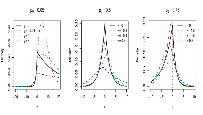
Figure 1: Density function of quantile-fixed generalized asymmetric Laplace distribution with $\mu=0$, $\sigma=1$ and different values of $\gamma$, for $p_{0}=0.05$, $0.5$ and $0.75$. In all cases, the solid line corresponds to the asymmetric Laplace density ($\gamma=0$).

The above connection between $(p_{0},\gamma)$ and $(p,\alpha)$ suggests that by reparameterization with desired $p_{0}$ and $\gamma=[I(\alpha>0)-p]|\alpha|$, we can derive a new family of distributions with the percentile for fixed $p_{0}$ given by $\mu$, and with an additional shape parameter $\gamma$. For $\gamma\neq 0$, the density, $f_{p_{0}}(y\mid\gamma,\mu,\sigma)$, of such quantile-fixed GAL distribution is

$$2\,\frac{p(1-p)}{\sigma}\left(\left\{\Phi\left(-\frac{p_{\gamma_{+}}y^{\ast}}{|\gamma|}+\frac{p_{\gamma_{-}}}{p_{\gamma_{+}}}|\gamma|\right)-\Phi\left(\frac{p_{\gamma_{-}}}{p_{\gamma_{+}}}|\gamma|\right)\right\}\exp\left\{-p_{\gamma_{-}}y^{\ast}+\frac{\gamma^{2}}{2}\left(\frac{p_{\gamma_{-}}}{p_{\gamma_{+}}}\right)^{2}\right\}I\left(\frac{y^{\ast}}{\gamma}>0\right)\right.$$ (5)

$$\qquad\qquad\qquad\qquad\qquad\qquad\qquad\qquad\left.+\,\Phi\left[-|\gamma|+\frac{p_{\gamma_{+}}y^{\ast}}{|\gamma|}I\left(\frac{y^{\ast}}{\gamma}>0\right)\right]\exp\left\{-p_{\gamma_{+}}y^{\ast}+\frac{\gamma^{2}}{2}\right\}\right)$$

where $p\equiv p(\gamma,p_{0})=$ $I(\gamma<0)+\{[p_{0}-I(\gamma<0)]/g(\gamma)\}$, $p_{\gamma_{+}}=$ $p-I(\gamma>0)$, $p_{\gamma_{-}}=$ $p-I(\gamma<0)$, and $y^{\ast}=$ $(y-\mu)/\sigma$. Parameter $\gamma$ has bounded support over interval $(L,U)$, where $L$ is the negative root of $g(\gamma)=1-p_{0}$ and $U$ is the positive root of $g(\gamma)=p_{0}$. For instance, $\gamma$ takes values in $(-0.07,15.90)$, $(-1.09,1.09)$ and $(-2.90,0.39)$ when $p_{0}=0.05$, $p_{0}=0.5$ and $p_{0}=0.75$, respectively. When $\gamma=0$, the density reduces to the AL density, which is also a limiting case of (5). The density function is continuous for all possible $\gamma$ values.

The quantile-fixed GAL distribution has three parameters, $\mu$, $\sigma$ and $\gamma$. Note that $Y$ has density $f_{p_{0}}(\cdot\mid\gamma,\mu,\sigma)$ if and only if $(Y-\mu)/\sigma$ has density $f_{p_{0}}(\cdot\mid\gamma,0,1)$. Hence, similarly to the AL distribution, $\mu$ is a location parameter and $\sigma$ is a scale parameter. The new shape parameter $\gamma$ enables the extension relative to the quantile-fixed AL distribution. As demonstrated in Figure 1, $\gamma$ controls skewness and tail behaviour, allowing for both left and right skewness when the median is fixed, as well as for both heavier and lighter tails than the asymmetric Laplace, the difference being particularly emphatic for extreme percentiles. Moreover, as $\gamma$ varies, the mode is no longer held fixed at $\mu$; it is less than $\mu$ when $\gamma<0$ and greater than $\mu$ when $\gamma>0$. The above attributes render the proposed distribution substantially more flexible than the AL distribution.

Finally, we note that parameter $\gamma$ satisfies likelihood identifiability. Consider the location-scale standardized density, $f_{p_{0}}(\cdot\mid\gamma,0,1)$, which is effectively the model for the errors in quantile regression. Then, assume $f_{p_{0}}(y\mid\gamma_{1},0,1)=$ $f_{p_{0}}(y\mid\gamma_{2},0,1)$, for all $y\in\mathbb{R}$. Given that parameter $\gamma$ controls the mode of the density, this implies that $\gamma_{1}$ and $\gamma_{2}$ must have the same sign. Working with either of the two cases (that is, $\gamma_{1}>0$ and $\gamma_{2}>0$ or $\gamma_{1}<0$ and $\gamma_{2}<0$) in expression (5), we arrive at $g(\gamma_{1})=$ $g(\gamma_{2})$, which, based on the monotonicity of function $g(\cdot)$, implies $\gamma_{1}=\gamma_{2}$.

3 Bayesian quantile regression with GAL errors

3.1 Inference for linear quantile regression

Consider continuous responses $y_{i}$ and the associated covariate vectors $\boldsymbol{x}_{i}$, for $i=1,\ldots,n$. The linear quantile regression model is set up as $y_{i}=$ $\boldsymbol{x}_{i}^{T}\boldsymbol{\beta}+\epsilon_{i}$, where the $\epsilon_{i}$ arise independently from a quantile-fixed GAL distribution with $\int_{-\infty}^{0}f_{p_{0}}(\epsilon\mid\gamma,0,\sigma)\mathrm{d}\epsilon=$ $p_{0}$. Owing to the mixture representation of the new distribution, the model for the data can be expressed hierarchically as follows

$$y_{i}\mid\boldsymbol{\beta},\gamma,\sigma,z_{i},s_{i} \stackrel{{\scriptstyle ind.}}{{\sim}} \text{N}(y_{i}\mid\boldsymbol{x}_{i}^{T}\boldsymbol{\beta}+\sigma C|\gamma|s_{i}+\sigma Az_{i},\sigma^{2}Bz_{i}),\,\,\,i=1,...,n$$

$$z_{i},s_{i} \stackrel{{\scriptstyle ind.}}{{\sim}} \text{Exp}(z_{i}\mid 1)\,\text{N}^{+}(s_{i}\mid 0,1),\,\,\,i=1,...,n$$ (6)

where $C=[I(\gamma>0)-p]^{-1}$, and $A$ and $B$ are the functions of $p$ given in (2). Since $p$ is a function of $\gamma$ and $p_{0}$, $A$, $B$ and $C$ are all functions of parameter $\gamma$. The Bayesian model is completed with priors for $\boldsymbol{\beta}$, $\sigma$ and $\gamma$. Here, we assume a normal prior $\text{N}(\boldsymbol{m}_{0},\Sigma_{0})$ for $\boldsymbol{\beta}$ and an inverse-gamma prior $\text{IG}(a_{\sigma},b_{\sigma})$ for $\sigma$, with mean $b_{\sigma}/(a_{\sigma}-1)$ provided $a_{\sigma}>1$. For any specified $p_{0}$, $\gamma$ is defined over an interval $(L,U)$ with fixed finite endpoints, and thus a natural prior for $\gamma$ is given by a rescaled Beta distribution, with the uniform distribution available as a default choice.

The augmented posterior distribution, which includes the $z_{i}$ and the $s_{i}$, can be explored via a Markov chain Monte Carlo algorithm based on Gibbs sampling updates for all parameters other than $\gamma$. As in Kozumi and Kobayashi (2011), we set $v_{i}=$ $\sigma z_{i}$, $i=1,\ldots,n$. Then, the posterior simulation method is based on the following updates.

• Sample $\boldsymbol{\beta}$ from $\text{N}(\boldsymbol{m}^{\ast},\Sigma^{\ast})$, with covariance matrix $\Sigma^{\ast}=$ $[\Sigma_{0}^{-1}+\sum_{i=1}^{n}\boldsymbol{x}_{i}\boldsymbol{x}_{i}^{T}/(B\sigma v_{i})]^{-1}$ and mean vector $\boldsymbol{m}^{\ast}=$ $\Sigma^{\ast}\{\Sigma_{0}^{-1}\boldsymbol{m}_{0}+\sum_{i=1}^{n}\boldsymbol{x}_{i}[y_{i}-(\sigma C|\gamma|s_{i}+Av_{i})]/(B\sigma v_{i})\}$.

• For each $i=1,...,n$, sample $v_{i}$ from a generalized inverse-Gaussian distribution, $\text{GIG}(0.5,a_{i},b_{i})$, where $a_{i}=[y_{i}-(\boldsymbol{x}_{i}^{T}\boldsymbol{\beta}+\sigma C|\gamma|s_{i})]^{2}/(B\sigma)$ and $b_{i}=2/\sigma+A^{2}/(B\sigma)$, with density given by $\text{GIG}(x\mid\nu,a,b)\propto$ $x^{\nu-1}\exp\{-0.5(a/x+bx)\}$.

• For each $i=1,...,n$, sample $s_{i}$ from a normal $\text{N}(\mu_{s_{i}},\sigma_{s_{i}}^{2})$ distribution truncated on $\mathbb{R}^{+}$, where $\sigma_{s_{i}}^{2}=$ $[(C\gamma)^{2}\sigma/(Bv_{i})+1]^{-1}$ and $\mu_{s_{i}}=$ $\sigma_{s_{i}}^{2}C|\gamma|[y_{i}-(\boldsymbol{x}_{i}^{T}\boldsymbol{\beta}+Av_{i})]/(Bv_{i})$.

• Sample $\sigma$ from a $\text{GIG}(\nu,c,d)$ distribution, where $\nu=$ $-(a_{\sigma}+1.5n)$, $c=$ $2b_{\sigma}+2\sum_{i=1}^{n}v_{i}+\sum_{i=1}^{n}[y_{i}-(\boldsymbol{x}_{i}^{T}\boldsymbol{\beta}+Av_{i})]^{2}/(Bv_{i})$, and $d=\sum_{i=1}^{n}(C\gamma s_{i})^{2}/(Bv_{i})$.

• Update $\gamma$ with a Metropolis-Hasting step, using a normal proposal distribution on the logit scale over $(L,U)$.

Based on the hierarchical model structure, the posterior predictive error density can be expressed as $p(\epsilon\mid\text{data})=$ $\int\text{N}(\epsilon\mid\sigma C|\gamma|s+\sigma Az,\sigma^{2}Bz)\,\text{Exp}(z\mid 1)\,\text{N}^{+}(s\mid 0,1)\,\pi(\gamma,\sigma\,|\,\mathrm{data})\,\mathrm{d}s\,\mathrm{d}z\,\mathrm{d}\gamma\,\mathrm{d}\sigma$, and thus estimated through Monte Carlo integration, using the posterior samples of $(\gamma,\sigma)$.

3.2 Quantile regression with regularization

Since the GAL distribution is constructed through modifying the mixture representation of the AL distribution, it retains some of the interesting properties of the AL distribution. In particular, working with the hierarchical representation of the GAL distribution, we are able to retrieve an extended version of the check loss function which corresponds to asymmetric Laplace errors.

Consider the collapsed posterior distribution, $\pi(\boldsymbol{\beta},\gamma,\sigma,s_{1},...,s_{n}\mid\text{data})$, that arises from (3.1) by marginalizing over the $z_{i}$. Then, the corresponding posterior full conditional for $\boldsymbol{\beta}$ can be expressed as

$$\pi(\boldsymbol{\beta}\mid\gamma,\sigma,s_{1},...,s_{n},\text{data})\propto\pi(\boldsymbol{\beta})\exp\left\{-\frac{1}{\sigma}\sum_{i=1}^{n}\rho_{p}(y_{i}-\boldsymbol{x}^{T}_{i}\boldsymbol{\beta}-\sigma H(\gamma)s_{i})\right\}$$

where $\pi(\boldsymbol{\beta})$ is the prior density for $\boldsymbol{\beta}$, $H(\gamma)=$ $\gamma g(\gamma)/\{g(\gamma)-|p_{0}-I(\gamma<0)|\}$, and $p=$ $I(\gamma<0)+\{[p_{0}-I(\gamma<0)]/g(\gamma)\}$, with $p_{0}$ the probability associated with the specified quantile modeled through $\boldsymbol{x}^{T}_{i}\boldsymbol{\beta}$. Hence, ignoring the prior contribution, finding the mode of the posterior full conditional for $\boldsymbol{\beta}$ is equivalent to minimizing with respect to $\boldsymbol{\beta}$ the adjusted loss function $\sum_{i=1}^{n}\rho_{p}(y_{i}-\boldsymbol{x}^{T}_{i}\boldsymbol{\beta}-\sigma H(\gamma)s_{i})$; note that in the special case with asymmetric Laplace errors, that is, for $\gamma=0$, this reduces to the check loss function with $p=$ $p_{0}$.

Based on the above structure, the positive-valued latent variables $s_{i}$ can be viewed as response-specific weights that are adjusted by real-valued coefficient $H(\gamma)$, which is fully specified through the shape parameter $\gamma$. The result is the real-valued, response-specific terms $\sigma H(\gamma)s_{i}$, which reflect on the estimation of $\boldsymbol{\beta}$ the effect of outlying observations relative to the AL distribution. A promising direction to further explore this structure is in the context of variable selection. For instance, Li et al. (2010) study connections between different versions of regularized quantile regression and different priors for $\boldsymbol{\beta}$, working with asymmetric Laplace errors. The main example is lasso regularized quantile regression, which can be connected to the Bayesian asymmetric Laplace error model through a hierarchical Laplace prior for $\boldsymbol{\beta}$. We consider this prior below extending the AL error distribution to the proposed GAL distribution. The perspective we offer may be useful, since it can be used to explore regularization adjusting the loss function, through the response distribution, in addition to the penalty term, through the prior for the regression coefficients.

Here, we denote by $\boldsymbol{\beta}$ the $d$-dimensional vector of regression coefficients excluding the intercept $\beta_{0}$. Then, the Laplace conditional prior structure for $\boldsymbol{\beta}$ is given by

$$\pi(\boldsymbol{\beta}\mid\sigma,\lambda)=\prod_{k=1}^{d}\frac{\lambda}{2\sigma}\exp\left\{-\frac{\lambda}{\sigma}|\beta_{k}|\right\}=\prod_{k=1}^{d}\int_{\mathbb{R}^{+}}\frac{1}{\sqrt{2\pi\omega_{k}}}\exp\left\{-\frac{\beta_{k}^{2}}{2\omega_{k}}\right\}\frac{\eta^{2}}{2}\exp\left\{-\frac{\eta^{2}}{2}\omega_{k}\right\}\,\mathrm{d}\omega_{k}.$$

The second expression above utilizes the normal scale mixture representation for the Laplace distribution, which has been exploited for posterior simulation in the context of lasso mean regression (Park and Casella, 2008). Moreover, to facilitate Markov chain Monte Carlo sampling, we reparameterize in terms of $\eta=$ $\lambda/\sigma$ and place a gamma prior on $\eta^{2}$. The lasso regularized version of model (3.1) is completed with a normal prior for $\beta_{0}$, and with the priors for the other parameters as given in Section 3.1. The posterior simulation algorithm is the same with the one described in Section 3.1 with the exception of the updates for the $\beta_{k}$, $k=1,...,d$, and for $\eta^{2}$. Using the mixture representation of the Laplace prior, each $\beta_{k}$ can be sampled from a normal distribution, whereas $\eta^{2}$ has a gamma posterior full conditional distribution.

3.3 Tobit quantile regression

Tobit regression offers a modeling strategy for problems involving range constraints on the response variable (Amemiya, 1984). The standard Tobit regression model can be viewed in the context of censored regression where the responses are left censored at a threshold $c$; without loss of generality, we take $c=0$. The responses can be written as $y_{i}=$ $\max\{0,y_{i}^{\ast}\}$, where $y_{i}$ are the observed values and $y_{i}^{\ast}$ are latent if $y_{i}^{\ast}\leq 0$. In the context of quantile regression, Yu and Stander (2007) and Kozumi and Kobayashi (2011) applied the AL-based model to the latent responses $y_{i}^{\ast}$. Here, we consider the Tobit quantile regression setting with GAL errors.

Consider a data set of $n+k$ observations on covariates and associated responses $\boldsymbol{y}=$ $(\boldsymbol{y}^{\mathrm{o}},\boldsymbol{0})$, where $\boldsymbol{y}^{\mathrm{o}}=$ $(y_{1}^{\mathrm{o}},...,y_{n}^{\mathrm{o}})$ consists of positive-valued observed responses with the remaining $k$ responses censored from below at $0$. Assuming the GAL distribution for the latent responses, the likelihood can be expressed as $\prod_{i=1}^{n}f_{p_{0}}(y_{i}^{\mathrm{o}}\mid\gamma,\boldsymbol{x}_{i}^{T}\boldsymbol{\beta},\sigma)\prod_{j=1}^{k}\int_{-\infty}^{0}f_{p_{0}}(w\mid\gamma,\boldsymbol{x}_{n+j}^{T}\boldsymbol{\beta},\sigma)\,\mathrm{d}w$. Using data augmentation (Chib, 1992), let $\boldsymbol{w}=$ $(w_{1},...,w_{k})$ be the unobserved (latent) responses corresponding to the $k$ data points that are left censored at $0$. Then, using again the hierarchical representation of the GAL distribution, the joint posterior distribution that includes $\boldsymbol{w}$ can be written as

$$\begin{array}[]{l}p(\boldsymbol{\beta},\gamma,\sigma,\{s_{i}\},\{v_{i}\},\boldsymbol{w}\mid\text{data})\propto\pi(\boldsymbol{\beta},\gamma,\sigma)\prod_{i=1}^{n}\text{N}(y_{i}^{\mathrm{o}}\mid\boldsymbol{x}_{i}^{T}\boldsymbol{\beta}+\sigma C|\gamma|s_{i}+Av_{i},\sigma Bv_{i})\\ \prod_{j=1}^{k}\text{N}^{-}(w_{j}\mid\boldsymbol{x}_{n+j}^{T}\boldsymbol{\beta}+\sigma C|\gamma|s_{n+j}+Av_{n+j},\sigma Bv_{n+j})\prod_{i=1}^{n+k}\,\text{Exp}(v_{i}\mid\sigma^{-1})\,\text{N}^{+}(s_{i}\mid 0,1)\end{array}$$

where $\pi(\boldsymbol{\beta},\gamma,\sigma)$ denotes the prior for the model parameters, and $v_{i}=$ $\sigma z_{i}$. Here, $\text{N}^{-}$ denotes a truncated normal on $\mathbb{R}^{-}$, and $\text{Exp}(v\,|\,\sigma^{-1})$ an exponential distribution with mean $\sigma$.

Regarding posterior inference, the posterior full conditional for each auxiliary variable $w_{j}$ is given by a truncated normal distribution. And, given the augmented data $(\boldsymbol{y}^{\mathrm{o}},\boldsymbol{w})$, the model parameters and the latent variables $\{(v_{i},s_{i}):i=1,...,n+k\}$ can be sampled as before.

Although results are not reported here, we have tested the posterior simulation algorithm on simulated data sets based on GAL errors, with $n=400$ observations and a censoring rate that ranged from $20\%$ to $40\%$. Under this scenario, the posterior distributions successfully captured the true values of all parameters in their 95% credible intervals.

4 Simulation study

Here, we present results from a simulation study designed to compare the lasso regularized quantile regression models with AL and GAL errors. We follow a standard simulation setting from the literature regarding the linear regression component (Tibshirani, 1996; Zou and Yuan, 2008; Li et al., 2010), varying the extent of sparsity in the true $\boldsymbol{\beta}$ vector. For the underlying data-generating error distributions, we consider four scenarios with different types of skewness and tail behavior. For model comparison, we evaluate the accuracy in variable selection, inference for the regression function, and posterior predictive performance, using relevant assessment criteria. Overall, the GAL-based quantile regression model performs better in variable selection and prediction accuracy and it is more robust to non-standard error distributions, particularly for extreme quantiles. The two models yield comparable results in the case of median regression.

4.1 Simulation settings

We consider synthetic data generated from linear quantile regression settings, with $p_{0}=0.05$, $0.25$ and $0.5$ to study model performance for both extreme and more central percentiles. The rows of the design matrix were generated independently from an 8-dimensional normal distribution with zero mean vector and covariance matrix with elements $0.5^{|i-j|}$, for $1\leq i,j\leq 8$. We present detailed results from a relatively sparse case for the vector of regression coefficients, $\boldsymbol{\beta}=$ $(3,1.5,0,0,2,0,0,0)$. In Section 4.3, we briefly discuss results form two other scenarios for $\boldsymbol{\beta}$ corresponding to a dense and a very sparse case.

Data were simulated under four different error distributions:

• $\mbox{N}(\mu,9)$, with $\mu$ chosen such that the $p_{0}$th quantile is 0.

• $\mbox{Laplace}(\mu,3)$, with $\mu$ chosen such that the $p_{0}$th quantile is 0.

• $0.1\mbox{N}(\mu,1)+0.9\mbox{N}(\mu+1,5)$, with $\mu$ chosen such that the $p_{0}$th quantile is 0.

• $\mbox{Log-transformed generalized Pareto}(\sigma,\xi)$, with $\xi=3$ and $\sigma$ chosen such that the $p_{0}$th quantile is 0. To generate the errors, we first sample from a generalized Pareto distribution, then take the logarithm. Based on the parameterization in Embrechts et al. (1997), the density function of the errors is given by $f(\epsilon\,|\,\sigma,\xi)=$ $\sigma^{-1}\{1+\xi\sigma^{-1}\exp(\epsilon)\}^{-(1+\xi^{-1})}\exp(\epsilon)$, for $\epsilon\in\mathbb{R}$.

The normal and Laplace error distributions are symmetric about zero under median regression. The parameters of the two-component normal mixture are selected such that the resulting error distribution is skewed. Finally, the log-transformed generalized Pareto distribution is included to study model performance under an error density which is both skewed and does not have exponential tails.

For each setting of the simulation study, we generated 100 data sets, each with $n=100$ observations for training the models and another $N=100$ for testing predictions.

4.2 Criteria for comparison

We consider a number of criteria to assess different aspects of model performance. Since Bayesian lasso regression only shrinks the covariate effects, we consider a threshold on the effect size for the purpose of variable selection. Following Hoti and Sillanpää (2006), we calculate the standardized effects as $\beta_{j}^{\ast}=$ $(s_{x_{j}}/s_{y})\beta_{j}$, $j=1,\ldots,d$, where $s_{x_{j}}$ is the standard deviation of predictor $x_{j}$ and $s_{y}$ is the standard deviation of the response. For each posterior sample, if the standardized effect is greater than 0.1 in absolute value, we consider the predictor as included. We count the number of correct inclusion and exclusions (CIE) in the posterior sample and divide it by $d$ to normalize it to a number between 0 and 1. By averaging over all the posterior samples, we obtain the mean standardized CIE for each simulated data set.

To assess predictive performance for the regression function, we calculate the mean check loss on the $N$ test data points, defined as: $\mathrm{MCL}=$ $N^{-1}\sum_{i=1}^{N}\rho_{p_{0}}(\boldsymbol{x}_{i}^{T}\boldsymbol{\beta}^{*}-\boldsymbol{x}_{i}^{T}\boldsymbol{\beta})$, where $\boldsymbol{\beta}^{*}$ is the posterior mean estimate from the training data. The mean check loss resembles the standard mean squared error criterion, which is commonly used for evaluating prediction with cross-validation.

Finally to assess model fitting taking into account predictive uncertainty, we apply the posterior predictive loss criterion from Gelfand and Ghosh (1998). This criterion favors the model $\mathcal{M}$ that minimizes $D_{m}(\mathcal{M})=$ $P(\mathcal{M})+\{m/(m+1)\}G(\mathcal{M})$, where $G(\mathcal{M})=$ $\sum_{i=1}^{n}\{y_{i}-\text{E}^{\mathcal{M}}(y^{*}_{i}\mid\text{data})\}^{2}$ is a goodness-of-fit term, and $P(\mathcal{M})=$ $\sum_{i=1}^{n}\text{var}^{\mathcal{M}}(y^{*}_{i}\mid\text{data})$ is a penalty term for model complexity. Here, $m\geq 0$, and $\text{E}^{\mathcal{M}}(y^{*}_{i}\mid\text{data})$ and $\text{var}^{\mathcal{M}}(y^{*}_{i}\mid\text{data})$ are the mean and variance under model $\mathcal{M}$ of the posterior predictive distribution for replicated response $y^{*}_{i}$ with corresponding covariate $\boldsymbol{x}_{i}$. We also consider the generalized version of the criterion based on the check loss function, under which $D(\mathcal{M})=$ $\sum_{i=1}^{n}\text{E}^{\mathcal{M}}(\rho_{p_{0}}(y_{i}-y^{*}_{i})\mid\text{data})$. For this generalized criterion, the goodness-of-fit term can be defined by $G(\mathcal{M})=$ $\sum_{i=1}^{n}\rho_{p_{0}}(y_{i}-\text{E}^{\mathcal{M}}(y^{*}_{i}\mid\text{data}))$ and the penalty term by $P(\mathcal{M})=$ $D(\mathcal{M})-G(\mathcal{M})$, since the check loss function $L(y,a)\equiv\rho_{p_{0}}(y-a)=$ $(y-a)p_{0}-(y-a)I(y<a)$ is convex in $y$, and thus $P(\mathcal{M})\geq 0$; see Gelfand and Ghosh (1998) for details on defining the model comparison criterion under loss functions different from quadratic loss.

4.3 Results

We used the same hierarchical Laplace prior for $\boldsymbol{\beta}$ under the AL and GAL models, with a gamma prior for $\eta^{2}$ with prior mean $1$ and variance $10$. Such prior specification is relatively non-informative in the sense that it does not favor shrinkage for the regression coefficients, resulting in marginal prior densities for each $\beta_{k}$ that place substantial probability mass away from $0$. The shape parameter $\gamma$ of the GAL error distribution was assigned a uniform prior. Results under both models and for each simulated data set are based on 5,000 posterior samples, obtained after discarding the first 50,000 iterations of the Markov chain Monte Carlo sampler and then retaining one every 20 iterations.

Within each simulation scenario, we summarize results from the 100 data sets using the median and standard deviation (SD) of the values for the performance assessment criteria discussed in Section 4.2. Results are reported in Table 1 through Table 4, where we use boldface to indicate the model supported by the particular criterion under each setting.

Overall, the lasso regularized Bayesian quantile regression model performs better under the GAL error distribution. The GAL-based model includes/excludes correct regression coefficient values more often than the AL model for almost all combinations of $p_{0}$ and error distributions (Table 1). It also results in a lower median mean check loss for the test data in most cases, demonstrating better performance in the prediction of the regression function (Table 2). Note that, for both types of assessment in Tables 1 and 2, the GAL-based model produces better results across all error distributions for $p_{0}=0.05$, and, with the exception of one case, when $p_{0}=0.25$. Results are generally more balanced in the median regression setting, although the GAL model fares better in all cases for which the underlying error distribution is skewed.

		Error distribution
					log-transformed
$p_{0}$	Model	Normal	Laplace	Normal mixture	generalized Pareto
0.05	GAL	0.848 (0.063)	0.633 (0.083)	0.911 (0.042)	0.893 (0.052)
	AL	0.746 (0.099)	0.534 (0.087)	0.817 (0.075)	0.840 (0.081)
0.25	GAL	0.851 (0.049)	0.728 (0.060)	0.918 (0.048)	0.896 (0.050)
	AL	0.843 (0.069)	0.700 (0.068)	0.913 (0.060)	0.900 (0.051)
0.50	GAL	0.848 (0.052)	0.738 (0.065)	0.909 (0.049)	0.897 (0.055)
	AL	0.850 (0.056)	0.737 (0.065)	0.905 (0.050)	0.870 (0.061)

Table 1: Simulation study. Standardized number of correctly included/excluded predictors: median (SD).

		Error distribution
					log-transformed
$p_{0}$	Model	Normal	Laplace	Normal mixture	generalized Pareto
0.05	GAL	0.340 (0.083)	1.073 (0.391)	0.224 (0.060)	0.268 (0.081)
	AL	0.523 (0.130)	1.709 (0.485)	0.375 (0.101)	0.388 (0.114)
0.25	GAL	0.325 (0.086)	0.676 (0.199)	0.225 (0.071)	0.265 (0.080)
	AL	0.360 (0.096)	0.778 (0.215)	0.257 (0.076)	0.274 (0.082)
0.50	GAL	0.323 (0.092)	0.642 (0.208)	0.235 (0.064)	0.262 (0.081)
	AL	0.322 (0.095)	0.624 (0.207)	0.237 (0.063)	0.294 (0.089)

Table 2: Simulation study. Mean check loss based on the test data: median (SD).

For each simulation setting, Table 3 includes the values for the posterior predictive loss criterion with quadratic loss (under $m\rightarrow\infty$, such that $D_{\infty}=$ $P+G$), and Table 4 shows the generalized criterion under check loss. Both versions of the posterior predictive loss criterion support the GAL model when $p_{0}=0.05$, with differences in values between the two models that are substantially larger than for the other two values of $p_{0}$. This reinforces the earlier findings on the potential benefits of the GAL error distribution for extreme percentiles. With the exception of one case under the check loss version of the criterion, the GAL-based model is also favored when $p_{0}=0.25$, whereas results are more mixed in the median regression case.

Finally, although detailed results are not reported here, the simulation study included two more settings for $\boldsymbol{\beta}$, a dense case with all $8$ regression coefficients equal to $0.85$, and a very sparse case with $\boldsymbol{\beta}=$ $(5,0,0,0,0,0,0,0)$. The conclusions were overall similar, in particular, the GAL model outperformed the AL model for essentially all combinations of underlying error distribution and value of $p_{0}=0.05$ or $p_{0}=0.25$. Again, in the median regression case, the distinction between the two models was less clear for the normal, Laplace and normal mixture data-generating distributions, although the GAL model performed better under all criteria for the setting corresponding to the log-transformed generalized Pareto distribution.

			Error distribution
						log-transformed
$p_{0}$	Model	Score	Normal	Laplace	Normal mixture	generalized Pareto
0.05	GAL	$P$	1231 (193)	9799 (2483)	653 (112)	1273 (270)
		$G$	832 (126)	7046 (1546)	429 (71)	1053 (267)
		$D_{\infty}$	2092 (312)	16860 (3839)	1085 (181)	2319 (531)
	AL	$P$	3359 (799)	30308 (10763)	1839 (405)	2782 (664)
		$G$	952 (165)	8659 (2304)	534 (93)	1168 (279)
		$D_{\infty}$	4357 (933)	38766 (12676)	2398 (487)	4020 (873)
0.25	GAL	$P$	1085 (206)	6977 (1607)	608 (95)	1445 (273)
		$G$	830 (146)	6897 (1606)	444 (66)	1105 (264)
		$D_{\infty}$	1882 (343)	13884 (3115)	1055 (154)	2552 (511)
	AL	$P$	1630 (303)	11503 (2727)	884 (148)	1516 (260)
		$G$	865 (154)	7395 (1742)	464 (71)	1113 (263)
		$D_{\infty}$	2499 (448)	18916 (4349)	1352 (215)	2600 (487)
0.50	GAL	$P$	1283 (205)	7600 (1676)	694 (97)	1189 (217)
		$G$	813 (132)	6459 (1509)	424 (60)	1089 (245)
		$D_{\infty}$	2111 (328)	14076 (3101)	1121 (152)	2283 (415)
	AL	$P$	1177 (191)	7256 (1572)	634 (87)	1318 (247)
		$G$	818 (134)	6431 (1509)	426 (60)	1107 (255)
		$D_{\infty}$	2008 (318)	13667 (3019)	1058 (143)	2415 (483)

Table 3: Simulation study. Penalty term ($P$), goodness-of-fit term ($G$) and posterior predictive loss criterion ($D_{\infty}$) under quadratic loss: median (SD).

		Error distribution
					log-transformed
$p_{0}$	Model	Normal	Laplace	Normal mixture	generalized Pareto
0.05	GAL	174.2 (13.6)	507.0 (67.8)	122.8 (11.3)	178.5 (17.4)
	AL	209.3 (21.7)	605.4 (70.8)	148.6 (17.3)	200.2 (20.5)
0.25	GAL	169.5 (15.9)	443.9 (47.1)	126.2 (9.5)	188.0 (17.5)
	AL	178.0 (15.7)	451.4 (45.8)	129.0 (9.8)	185.5 (17.3)
0.50	GAL	175.7 (13.4)	444.7 (48.0)	127.4 (8.9)	178.6 (16.1)
	AL	172.6 (13.4)	438.5 (47.5)	125.2 (8.7)	183.6 (18.1)

Table 4: Simulation study. Posterior predictive loss criterion under check loss: median (SD).

5 Data examples

In this section, we consider three data examples to illustrate the Bayesian quantile regression models developed in Sections 3.1, 3.2, and 3.3. The main emphasis is on comparison of inference results between models based on the GAL distribution and those assuming an AL distribution for the errors.

We have implemented both models with priors for their parameters that result in essentially the same prior predictive error densities. The two models were applied with the same prior distributions for $\boldsymbol{\beta}$ and $\sigma$. More specifically, for the data sets of Sections 5.1 and 5.3, we used a $\text{N}(\boldsymbol{0},100I)$ prior for the vector of regression coefficients, and an $\text{IG}(2,2)$ prior for the scale parameter $\sigma$. For the data example of Section 5.2, we used a $\text{N}(0,100)$ prior for the intercept, and the same conditional Laplace prior for the remaining regression coefficients with the simulation study (see Section 4.3). Finally, a uniform prior was placed on the shape parameter $\gamma$ of the GAL error distribution. For all data examples, the posterior densities for model parameters were fairly concentrated relative to the corresponding prior densities.

5.1 Immunoglobulin-G data

We illustrate the proposed model, referred to as model $\text{M}_{1}$, with a data set commonly used in additive quantile regression; see, for instance, Yu and Moyeed (2001). The analysis focuses on comparison with the simpler model based on asymmetric Laplace errors, referred to as model $\text{M}_{0}$. The data set contains the immunoglobulin-G concentration in grams per litre for $n=298$ children aged between 6 months and 6 years. As in earlier applications of quantile regression for these data, we use a quadratic regression function $\beta_{0}+\beta_{1}x+\beta_{2}x^{2}$ to model five quantiles, corresponding to $p_{0}=$ $0.05,\,0.25,\,0.5,\,0.75,\,0.95$, of immunoglobulin-G concentration against covariate age ($x$).

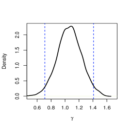
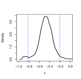
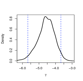
Figure 2: Immunoglobulin-G data. Inference results for $p_{0}=0.25$, $0.5$ and $0.95$. Top row: posterior predictive error densities under the asymmetric Laplace model (dashed lines) and the generalized asymmetric Laplace model (solid lines). Bottom row: posterior densities for parameter $\gamma$, with the vertical lines corresponding to the endpoints of the 95% credible interval.

The two models result in different posterior predictive error densities, especially for extreme percentiles; see Figure 2. At $p_{0}=$ $0.95$, under the AL model, both the shape and the skewness of the error distribution are predetermined by $p_{0}$ and the mode is forced to be 0, resulting in a rigid heavy left tail. The effect of this overly dispersed tail can be observed in the inference for the quantile regression function (Figure 3). The GAL model, on the contrary, yields an error density that has a much thinner left tail, concentrating more of its probability mass around the mode, which is not at 0. Figure 2 shows also the posterior densities for shape parameter $\gamma$, under a uniform prior in all cases. For all three quantile regressions, the 95% posterior credible interval for $\gamma$ does not include the value of 0, which corresponds to asymmetric Laplace errors. Median regression is the only case where 0 is within the effective range of the posterior distribution for $\gamma$.

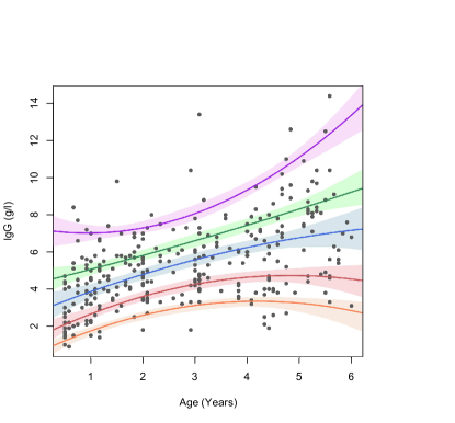
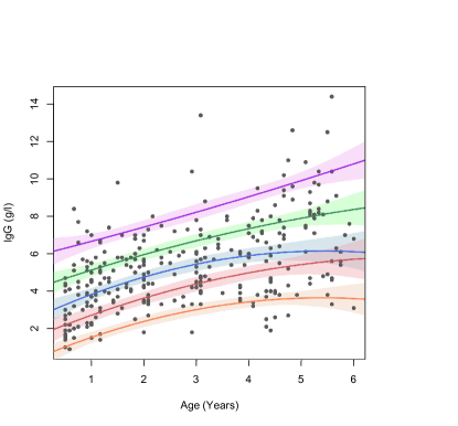
Figure 3: Immunoglobulin-G data. Posterior mean estimates and 95% credible bands for the quantile regression function $\beta_{0}+\beta_{1}x+\beta_{2}x^{2}$ against age ($x$), for $p_{0}=$ 0.05, 0.25, 0.50, 0.75 and 0.95. Left: AL model. Right: GAL model.

		Bayesian information criterion
Quantile	Model	log-likelihood	BIC
$~{}p_{0}=0.05~{}~{}$	$\text{M}_{0}$	$-666$	$1355$
	$\text{M}_{1}$	$-615$	$1258$
$~{}p_{0}=0.25$	$\text{M}_{0}$	$-632$	$1287$
	$\text{M}_{1}$	$-622$	$1273$
$~{}p_{0}=0.50$	$\text{M}_{0}$	$-633$	$1289$
	$\text{M}_{1}$	$-623$	$1274$
$~{}p_{0}=0.75$	$\text{M}_{0}$	$-654$	$1331$
	$\text{M}_{1}$	$-620$	$1268$
$~{}p_{0}=0.95$	$\text{M}_{0}$	$-761$	$1545$
	$\text{M}_{1}$	$-646$	$1320$

Table 5: Immunoglobulin-G data. Bayesian information criterion under the asymmetric Laplace and generalized asymmetric Laplace models, denoted by $\text{M}_{0}$ and $\text{M}_{1}$, respectively.

For formal model comparison, we compute the Bayesian information criterion (BIC), the posterior predictive loss criterion with quadratic loss, and the generalized posterior predictive loss criterion under the check loss. The Bayesian information criterion favors the new model at all five quantiles; see Table 5. Under the posterior predictive loss criterion (Table 6), the two models are comparable in the case of median regression, with model $\text{M}_{0}$ preferred. In all other cases, model $\text{M}_{1}$ is favored by both versions of the model comparison criterion. The improvement in performance over the AL model is particularly conspicuous at the two extreme percentiles. This is in agreement with the difference in the posterior predictive error densities for $p_{0}=0.95$, reported in Figure 2.

		Posterior predictive loss criterion
		Quadratic loss				Check loss
Quantile	Model	P	G	D∞		P	G	D
$~{}p_{0}=0.05~{}~{}$	$\text{M}_{0}$	$3511$	$1331$	$4841$		$179$	$180$	$359$
	$\text{M}_{1}$	$1298$	$1170$	$2467$		$230$	$102$	$331$
$~{}p_{0}=0.25$	$\text{M}_{0}$	$1820$	$1180$	$3001$		$232$	$123$	$355$
	$\text{M}_{1}$	$1407$	$1144$	$2551$		$236$	$108$	$343$
$~{}p_{0}=0.50$	$\text{M}_{0}$	$1465$	$1142$	$2607$		$229$	$108$	$338$
	$\text{M}_{1}$	$1626$	$1161$	$2788$		$232$	$114$	$346$
$~{}p_{0}=0.75$	$\text{M}_{0}$	$2122$	$1227$	$3350$		$201$	$134$	$335$
	$\text{M}_{1}$	$1208$	$1140$	$2348$		$228$	$97$	$325$
$~{}p_{0}=0.95$	$\text{M}_{0}$	$6522$	$1751$	$8273$		$137$	$259$	$395$
	$\text{M}_{1}$	$1525$	$1165$	$2690$		$208$	$118$	$327$

Table 6: Immunoglobulin-G data. Posterior predictive loss criterion (based on quadratic loss and check loss functions) under the asymmetric Laplace and generalized asymmetric Laplace models, denoted by $\text{M}_{0}$ and $\text{M}_{1}$.

5.2 Boston housing data

We apply the lasso regularized quantile regression model to the realty price data from the Boston Standard Metropolitan Statistical Area (SMSA) in 1970 (Harrison and Rubinfeld, 1978). The data set contains 506 observations. We take the log-transformed corrected median value of owner-occupied housing in USD 1000 (LCMEDV) as the response, and consider the following predictors: point longitudes in decimal degrees (LON), point latitudes in decimal degrees (LAT), per capita crime (CRIM), proportions of residential land zoned for lots over 25000 square feet per town (ZN), proportions of non-retail business acres per town (INDUS), a factor indicating whether tract borders Charles River (CHAS), nitric oxides concentration (parts per 10 million) per town (NOX), average numbers of rooms per dwelling (RM), proportions of owner-occupied units built prior to 1940 (AGE), weighted distances to five Boston employment centers (DIS), index of accessibility to radial highways per town (RAD), full-value property-tax rate per USD 10,000 per town (TAX), pupil-teacher ratios per town (PTRATIO), transformed African American population proportion (B), and percentage values of lower status population (LSTAT).

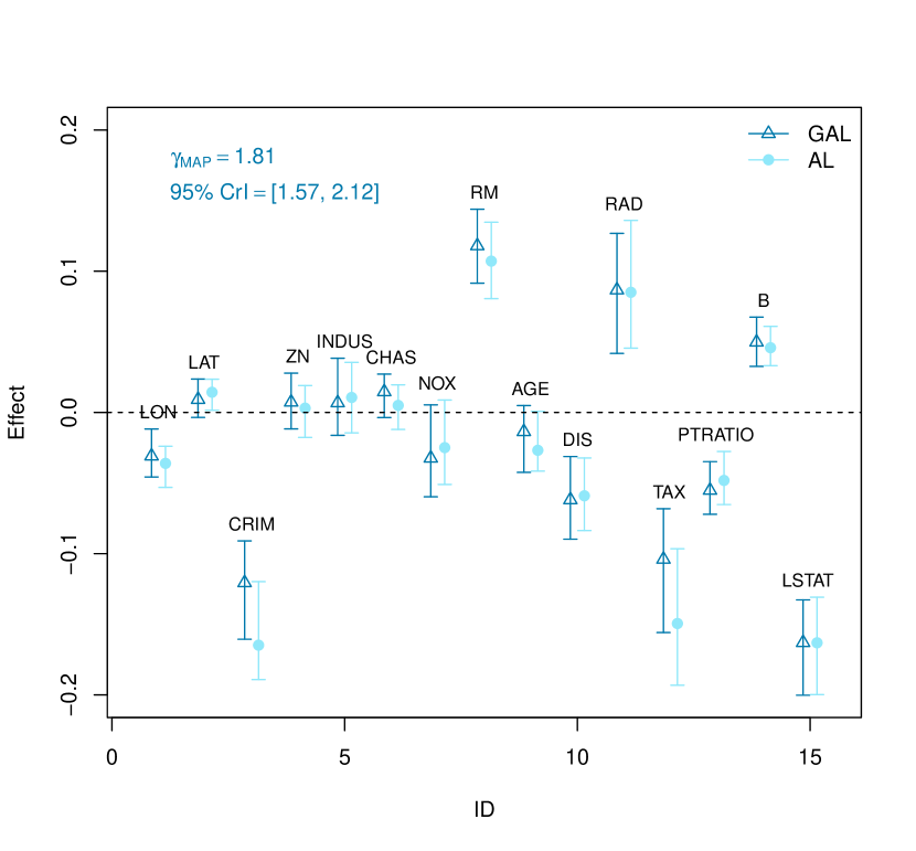
Figure 4: Boston housing data. Posterior point and 95% interval estimates for the regression coefficients of the 10th quantile lasso regularized model under AL and GAL errors.

We consider quantiles of $0.1$ and $0.9$ and compare the maximum a posteriori estimates (MAP) of regression coefficients, along with 95% credible intervals, for standardized covariates under the lasso regularized quantile regression models with AL and GAL errors (Figure 4 and 5). For both quantiles, the widths of the 95% credible intervals for the regression coefficients are overall comparable between the two models, but the posterior point estimates can be quite different. For instance, under the 10th quantile regression, the GAL model shrinks the effects of per capita crime (CRIM) and proporty-tax rate (TAX) to a greater extent compared to the AL model. Similar patterns can be observed for index of accessibility to radial highways (RAD) for the 90th quantile. Moreover, the two models reach different conclusions on the effect of latitude (LAT) for the 10th percentile. Although the posterior point estimates suggest a higher housing price as latitude increases adjusting for all other covariates, the 95% credible interval under the GAL model includes 0, whereas the one under the AL model does not.

Focusing on inference under the GAL error distribution, we note that, although the model selected some common variables for the two quantiles, there is also some discrepancy. For instance, each of higher proportions of residential land zoned for lots over 25000 square feet per town (ZN) and having tracts bordering Charles river (CHAS) increase the price at the 90% percentile, while higher nitrogen oxide value (NOX) has a negative influence on the 90% percentile price. However, none of these covariates have a significant effect on the realty value at the 10% percentile.

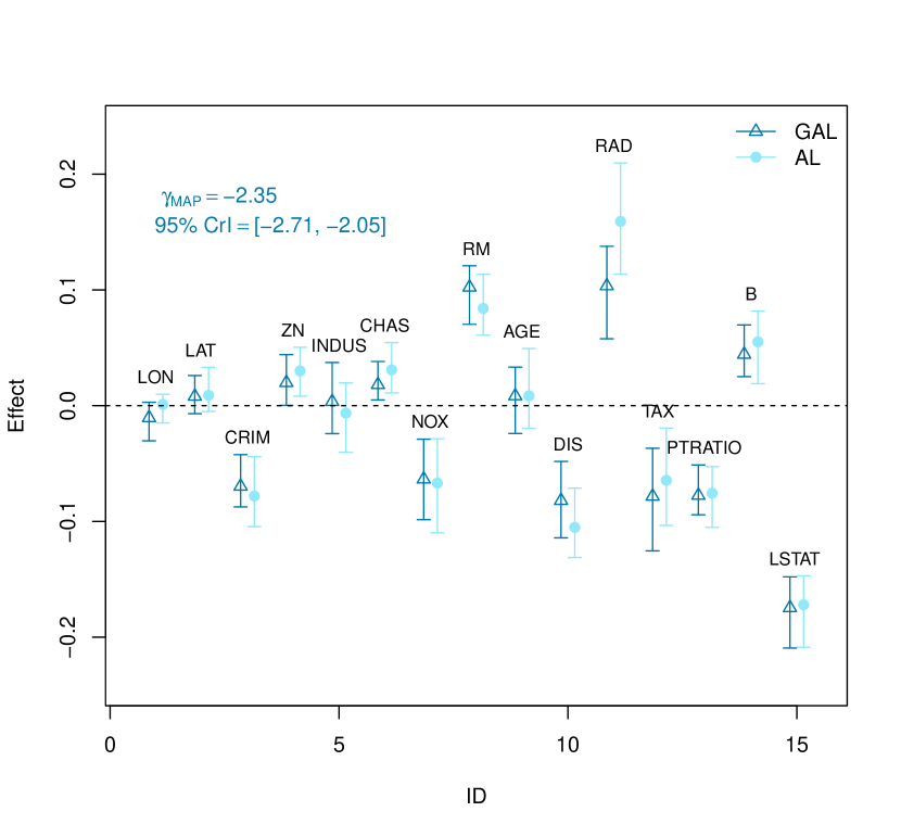
Figure 5: Boston housing data. Posterior point and 95% interval estimates for the regression coefficients of the 90th quantile lasso regularized model under AL and GAL errors.

Finally, we notice that for both the 10th and 90th quantile regression, 0 is far away from the endpoints of the 95% credible interval for the GAL model shape parameter $\gamma$. This suggests that asymmetric Laplace errors are not suitable for this particular application. This is further supported by the results for the posterior predictive loss criterion reported in Table 7.

		Posterior predictive loss criterion
		Quadratic loss				Check loss
Quantile	Model	P	G	D∞		P	G	D
$~{}p_{0}=0.10~{}~{}$	$\text{M}_{0}$	$46.9$	$26.2$	$73.1$		$28.1$	$22.6$	$50.7$
	$\text{M}_{1}$	$22.8$	$20.1$	$42.9$		$30.4$	$18.5$	$48.9$
$~{}p_{0}=0.90$	$\text{M}_{0}$	$74.8$	$28.8$	$103.6$		$24.1$	$31.5$	$55.7$
	$\text{M}_{1}$	$22.6$	$18.4$	$41.0$		$26.3$	$21.0$	$47.3$

Table 7: Boston housing data. Posterior predictive loss criterion (based on quadratic loss and check loss functions) under the AL (model $\text{M}_{0}$) and GAL (model $\text{M}_{1}$) error distribution.

5.3 Labor supply data

We illustrate the Tobit quantile regression model with the female labor supply data from Mroz (1987), which was taken from the University of Michigan Panel Study of Income Dynamics for year 1975. The data set includes records on the work hours and other relevant information of $753$ married white women aged between 30 and 60 years old. Of the $753$ women, $428$ worked at some time during 1975, with the corresponding fully observed responses given by the wife’s work hours (in 100 hours). For the remaining $325$ women, the observed zero work hours correspond to negative values for the latent “labor supply” response. We use the quantile regression function considered in Kozumi and Kobayashi (2011), where an AL-based Tobit quantile regression model was applied to the same data set. The linear predictor includes an intercept, income which is not due to the wife (nwifeinc), education of the wife in years (educ), actual labor market experience in years (exper) and its quadratic term (expersq), age of the wife (age), number of children less than 6 years old in household (kidslt6), and number of children between ages 6 and 18 in household (kidsge6). We compare the results from the Bayesian Tobit quantile regression model assuming AL errors (model $\text{M}_{0}$) and GAL errors (model $\text{M}_{1}$).

Table 8 summarizes the posterior distribution of $\gamma$ under the GAL model, and presents results from criterion-based comparison of the two models for $p_{0}=0.05$, $0.50$ and $0.95$. Since there is censoring in the data, we use the revised BIC from Volinsky and Raftery (2000). In all three cases, the 95% credible interval for $\gamma$ excludes $0$, and the GAL-based model is associated with lower BIC values. The results support the GAL-based model more emphatically for the extreme percentiles than for median regression.

Quantile	Model	Mean (95% CrI) for $\gamma$	likelihood	BIC
$~{}p_{0}=0.05$	$\text{M}_{0}$		$-1975$	$4004$
	$\text{M}_{1}$	$5.22$ ($4.43$, $6.24$)	$-1874$	$3809$
$~{}p_{0}=0.50$	$\text{M}_{0}$		$-1867$	$3789$
	$\text{M}_{1}$	$0.58$ ($0.39$, $0.81$)	$-1845$	$3750$
$~{}p_{0}=0.95$	$\text{M}_{0}$		$-1967$	$3989$
	$\text{M}_{1}$	$-4.16$ ($-5.5$, $-3.06$)	$-1854$	$3769$

Table 8: Labor supply data. Posterior mean and 95% credible interval for the shape parameter $\gamma$ of the GAL error distribution, and BIC values under the AL and GAL models, denoted by $\text{M}_{0}$ and $\text{M}_{1}$, respectively.

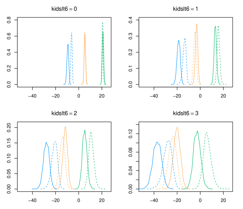
Figure 6: Labor supply data. Posterior densities for the 5th (blue), 50th (orange) and 95th quantile (green) of labor supply (in 100 hours) for women with 0, 1, 2 or 3 children less than 6 years old. The solid (dashed) lines correspond to the posterior densities under the GAL (AL) model.

Figure 6 shows the posterior distributions of labor supply quantiles corresponding to $p_{0}=0.05$, $0.50$ and $0.95$ for women with 0, 1, 2 and 3 children less than 6 years old. For all other predictors, we use the median values from the data as input values to represent an average wife. As the number of young children increases, the AL model estimates the 5th quantile and the median of labor supply of an average wife to be closer to each other. Under the GAL model, the distance between the densities of the 5th quantile and median labor supply also decreases with increasing number of young children, albeit at a lower rate. When estimating the 95th quantile, the proposed model is more conservative than the AL model about the labor contribution of an average wife with an increasing number of children less than 6 years old. When there are 3 children less than 6 years old in the household, the center of the posterior distribution for the 95th quantile is below zero under the GAL model, meaning that even at the top 5th percentile of labor supply, an average wife may still produce negative labor supply as she takes care of many young family members. More specifically, the posterior probability of the 95th labor supply quantile being positive is 0.19 under the GAL model, as opposed to 0.97 under the AL model. These results demonstrate that the choice of error distribution in quantile regression can have an effect on practically important conclusions for a particular application.

6 Discussion

We have developed a Bayesian quantile regression framework with a new error distribution that has flexible skewness, mode and tail behavior. The proposed model has better performance compared with the commonly used asymmetric Laplace distribution, particularly for modeling extreme quantiles. Owing to the hierarchical structure of the new distribution, posterior inference and prediction can be readily implemented via Markov chain Monte Carlo methods.

The main motivation for this work was to develop a sufficiently flexible parametric distribution that can be used as a building block for different types of quantile regression models. The extension to quantile regression with ordinal responses is a possible direction. Expanding the model to a spatial quantile regression process, along the lines of Lum and Gelfand (2012), is another direction. Finally, current work is exploring a composite quantile regression modeling framework, built from structured mixtures of generalized asymmetric Laplace distributions, to combine information from multiple quantiles of the response distribution in inference for variable selection.

References

- Amemiya (1984) Amemiya, T. (1984), “Tobit models: A survey,” Journal of econometrics, 24, 3–61.
- Azzalini (1985) Azzalini, A. (1985), “A class of distributions which includes the normal ones,” Scandinavian Journal of Statistics, 12, 171–178.
- Chib (1992) Chib, S. (1992), “Bayes inference in the Tobit censored regression model,” Journal of Econometrics, 51, 79–99.
- Embrechts et al. (1997) Embrechts, P., Klüppelberg, C., and Mikosch, T. (1997), Modelling extremal events, vol. 33, Springer Science & Business Media.
- Gelfand and Ghosh (1998) Gelfand, A. and Ghosh, S. (1998), “Model choice: A minimum posterior predictive loss approach,” Biometrika, 85, 1–11.
- Hanson and Johnson (2002) Hanson, T. and Johnson, W. O. (2002), “Modeling regression error with a mixture of Pólya trees.” Journal of the American Statistical Association, 97, 1020–1033.
- Harrison and Rubinfeld (1978) Harrison, D. and Rubinfeld, D. L. (1978), “Hedonic housing prices and the demand for clean air,” Journal of environmental economics and management, 5, 81–102.
- Henze (1986) Henze, N. (1986), “A probabilistic representation of the skew-normal distribution,” Scandinavian Journal of Statistics, 13, 271–275.
- Hoti and Sillanpää (2006) Hoti, F. and Sillanpää, M. (2006), “Bayesian mapping of genotype expression interactions in quantitative and qualitative traits,” Heredity, 97, 4–18.
- Koenker (2005) Koenker, R. (2005), Quantile Regression, New York: Cambridge University Press.
- Kottas and Gelfand (2001) Kottas, A. and Gelfand, A. E. (2001), “Bayesian semiparametric median regression modeling,” Journal of the American Statistical Association, 96, 1458–1468.
- Kottas and Krnjajić (2009) Kottas, A. and Krnjajić, M. (2009), “Bayesian semiparametric modelling in quantile regression,” Scandinavian Journal of Statistics, 36, 297–319.
- Kotz et al. (2001) Kotz, S., Kozubowski, T., and Podgorski, K. (2001), The Laplace Distribution and Generalizations: A Revisit With Applications to Communications, Exonomics, Engineering, and Finance, Boston: Birkhäuser.
- Kozumi and Kobayashi (2011) Kozumi, H. and Kobayashi, G. (2011), “Gibbs sampling methods for Bayesian quantile regression,” Journal of Statistical Computation and Simulation, 81, 1565–1578.
- Li et al. (2010) Li, Q., Xi, R., and Lin, N. (2010), “Bayesian regularized quantile regression,” Bayesian Analysis, 5, 533–556.
- Lum and Gelfand (2012) Lum, K. and Gelfand, A. E. (2012), “Spatial quantile multiple regression using the asymmetric Laplace process (with discussion),” Bayesian Analysis, 7, 235–276.
- Mroz (1987) Mroz, T. A. (1987), “The sensitivity of an empirical model of married womenś hours of work to economic and statistical assumptions,” Econometrica: Journal of the Econometric Society, 765–799.
- Park and Casella (2008) Park, T. and Casella, G. (2008), “The Bayesian lasso,” Journal of the American Statistical Association, 103, 681–686.
- Reich et al. (2010) Reich, B. J., Bondell, H. D., and Wang, H. J. (2010), “Flexible Bayesian quantile regression for independent and clustered data,” Biostatistics, 11, 337–352.
- Reich and Smith (2013) Reich, B. J. and Smith, L. B. (2013), “Bayesian quantile regression for censored data,” Biometrics, 69, 651–660.
- Taddy and Kottas (2010) Taddy, M. and Kottas, A. (2010), “A Bayesian nonparametric approach to inference for quantile regression,” Journal of Business and Economic Statistics, 28, 357–369.
- Tibshirani (1996) Tibshirani, R. (1996), “Regression shrinkage and selection via the lasso,” Journal of the Royal Statistical Society. Series B (Methodological), 267–288.
- Tokdar and Kadane (2012) Tokdar, S. T. and Kadane, J. B. (2012), “Simultaneous linear quantile regression: A semiparametric Bayesian approach,” Bayesian Analysis, 7, 51–72.
- Tsionas (2003) Tsionas, E. G. (2003), “Bayesian quantile inference,” Journal of Statistical Computation and Simulation, 73, 659–674.
- Volinsky and Raftery (2000) Volinsky, C. T. and Raftery, A. E. (2000), “Bayesian information criterion for censored survival models,” Biometrics, 56, 256–262.
- Waldmann et al. (2013) Waldmann, E., Kneib, T., Yue, Y. R., Lang, S., and Flexeder, C. (2013), “Bayesian semiparametric additive quantile regression,” Statistical Modelling, 13, 223–252.
- Walker and Mallick (1999) Walker, S. G. and Mallick, B. K. (1999), “A Bayesian semiparametric accelerated failure time model,” Biometrics, 55, 477–483.
- Wichitaksorn et al. (2014) Wichitaksorn, N., Choy, B. S. T., and Gerlach, R. (2014), “A generalized class of skew distributions and associated robust quantile regression models,” The Canadian Journal of Statistics, 42, 579–596.
- Yu and Moyeed (2001) Yu, K. and Moyeed, R. A. (2001), “Bayesian quantile regression,” Statistics & Probability Letters, 54, 437–447.
- Yu and Stander (2007) Yu, K. and Stander, J. (2007), “Bayesian analysis of a Tobit quantile regression model,” Journal of Econometrics, 137, 260–276.
- Zhu and Galbraith (2011) Zhu, D. and Galbraith, J. W. (2011), “Modeling and forecasting expected shortfall with the generalized asymmetric Student-t and asymmetric exponential power distributions,” Journal of Empirical Finance, 18, 765–778.
- Zhu and Zinde-Walsh (2009) Zhu, D. and Zinde-Walsh, V. (2009), “Properties and estimation of asymmetric exponential power distribution,” Journal of Econometrics, 148, 86–99.
- Zou and Yuan (2008) Zou, H. and Yuan, M. (2008), “Composite quantile regression and the oracle model selection theory,” The Annals of Statistics, 36, 1108–1126.