Eccentricity in planetary systems and the role of binarity

We explore the multiplicity of exoplanet host stars with high-resolution images obtained with VLT/SPHERE. Two different samples of systems were observed: one containing low-eccentricity outer planets, and the other containing high-eccentricity outer planets. We find that 10 out of 34 stars in the high-eccentricity systems are members of a binary, while the proportion is 3 out of 27 for circular systems. Eccentric-exoplanet hosts are, therefore, significantly more likely to have a stellar companion than circular-exoplanet hosts. The median magnitude contrast over the 68 data sets is 11.26 and 9.25, in H and K, respectively, at 0.30 arcsec. The derived detection limits reveal that binaries with separations of less than 50au are rarer for exoplanet hosts than for field stars. Our results also imply that the majority of high-eccentricity planets are not embedded in multiple stellar systems (24 out of 34), since our detection limits exclude the presence of a stellar companion. We detect the low-mass stellar companions of HD 7449 and HD 211847, both members of our high-eccentricity sample. HD 7449B was already detected by Rodigas et al. (2016) and our independent observation is in agreement with this earlier work. HD 211847’s substellar companion, previously detected by the radial velocity method, is actually a low-mass star seen face-on. The role of stellar multiplicity in shaping planetary systems is confirmed by this work, although it does not appear as the only source of dynamical excitation.

1 Introduction

The distribution of eccentricities amongst the exoplanet population discovered by the radial-velocity method is intriguing, as nearly circular orbits such as those in the solar system coexist with much more eccentric ones. Approximately 12% of these RV planets have eccentricities more than 0.5 and 45% have eccentricities larger than 0.2, which is the maximum eccentricity in the solar system (Mercury). Where planets mostly formed via the core-accretion mechanism in the central part of circumstellar disks, little dynamical excitation is expected (Pollack et al., 1996), and simulations of young planetary systems have a clear tendency for coplanarity, circularity, and minimum energy exchange between planets. However, models now exist for more excited systems implying planet-planet scattering (Chatterjee et al., 2008), dynamical interactions with a distant stellar companion, and/or the Kozai resonance mechanism (Naoz et al., 2012; Wu et al., 2007; Kozai, 1962). This Kozai mechanism involves the gravitational interaction between a planet and an outer stellar companion that is orbiting at large separations (up to several hundred au) from the central star. The gravitational interactions between both objects induces Kozai oscillations, which gradually pump the planetary orbit to high eccentricity and inclinations while tidal dissipation from the central star circularizes the orbit (Wu et al., 2007). For tighter binaries, it is the secular perturbations of the secondary that can force high eccentricities on circumprimary planets (see for ex. HD 41004 or HD 196885, Thebault (2011a)).

Simulating the dynamical evolution of planetary systems requires the global knowledge of all components of the system and the presence of a distant stellar companion is evidently a significant piece of information improving the accuracy of a model. It is expected from theory that binaries with separations $<$50au should have a strong impact on planet formation around the primary (Thebault & Haghighipour, 2014). However, observations have revealed that some binaries as tight as 20au indeed harbor planets ($\gamma$ Cephei, HD 196885). Discovering new planet-harboring tight binaries is therefore essential to our understanding of how planet formation unfolds in such extreme conditions. Unfortunately, the stellar multiplicity is generally not known at the time of discovering a new planet with the RV method even though it may seem trivial compared to the planet discovery: while equal-mass short-period binaries are discarded by immediate spectroscopic analysis, long-period stellar companions are more difficult to recognize since their signatures may take tens of years to reveal themselves. For instance, a 0.1 solar mass companion located on a 10⁵-day orbit from a solar-type star has a semi-amplitude of 60 m/s over 274 years equivalent to non-detectable trend over the typical 2-3 years of RV monitoring. Such secondary components, however, would be located at 0.4” for a 100pc distance system and would have a magnitude difference of six in the H band, making them detectable in direct imaging with instruments such as VLT/SPHERE (Beuzit et al., 2008) that provide high-contrast capabilities within one arcsecond.

Determining any correlation between eccentric systems and the presence of distant massive companions would directly test the formation/migration mechanisms. In addition, peculiar systems with detection of secondary components could be scrutinized with dedicated modeling, as done for $\alpha$ Cen or HD196885 (Thébault et al., 2009; Thebault, 2011b).

Several imaging programs have observed exoplanet-hosting stars in the past. For instance, Mugrauer et al. (2014a) and references therein presented SOFI imaging observations of such systems; their observations probed the separations of 30 to 200 arcsec revealing that 13% of exoplanet host stars in their sample contained distant stellar companions. Narita et al. (2012) discovered the stellar companion to HAT-P-7 (with a magnitude difference of approximately six and 3.9” separation) using Subaru IRCS and HiCIAO and were able to revisit the migration history of this system. Ngo et al. (2016) focused on the stellar companions of hot-Jupiter systems and found that wide stellar companions were in excess compared to field stars. The objective of this work is to assess the presence of any stellar companion in the separation range 0.1–4 arcsec and mass regime $>$ 0.06 solar mass around all targets in two samples, and to statistically compare them. In Section 2, we describe the sample selection and strategy. In Section 3, we present the new data set of VLT/SPHERE high-contrast imaging. In Section 4, we present and discuss candidate detections for all systems with a particular emphasis on HD 7449 and HD 211847, which both present short-separation companions. Where no companion is found, we discuss and quantify detection limits. We conclude in Section 5.

Figure 1: Eccentricity as a function of minimum companion mass of the systems where these parameters are known (open circles), and of the sample of systems considered in this study (filled circles).

2 The sample

We have selected all exoplanets in a volume of 100 pc, with host stars brighter than V magnitude of nine, that are able to be observed from the Paranal Observatory (Chile). In this sample we made two groups: planets with very high eccentricity (e$>$0.4, 35 systems) and circular planets (e$<$0.05, 27 systems). We a priori discarded the systems with intermediate eccentricities, which amounted to 205. When several planets were present in a system (there are 17 multi-planet systems in total) we attribute the system to one sample or the other according to the eccentricity of the outermost planet, since it is the one most susceptible to the effect of massive companions at further distances. We have listed relevant parameters of systems in Tables 1 and 2 and their distribution in the planet mass-eccentricity diagram is shown in Fig. 1. Errors on the parameters are not replicated in these tables but can be found in the Exoplanet Encyclopedia. Note that three additional systems were observed, HD 47186, HD 92788, and HD 168443, which were originally put in the comparison sample, but for which the outermost planet has intermediate eccentricity and does not fulfill any of our criteria anymore (they were misclassified or updated). However, since they were observed their data has been included in the reduction and analysis. Their parameters are given in the bottom lines of Table 2.

The magnitude limit is set to allow the full sample to be observed in a short time as a bad-weather filler program using VLT/SPHERE to either confirm or reject the presence of outer, massive companions, focusing on the closest separation range.

It is interesting to note that the comparison sample contains much more multi-planet systems than the ”eccentric sample” (ten vs. four): this is, however, expected due to dynamical interactions (e.g., Lissauer et al., 2011) and/or detection biases in radial-velocity surveys. A similar observation was made by Desidera & Barbieri (2007).

Table 1: System parameters for the ”eccentric” sample. The selection is based on the eccentricity of the outermost planet. The object with an asterisk ^∗ is actually not a planetary but a stellar companion (see text). There is one line per planet. The age is not always estimated.

Name	mH	Minimum Mp	$e$	Period	$a$	Ms	Dist	Age
		MJup		days	au	M⊙	pc	Gy
GJ 3021	4.99	3.37	0.51	133.71	0.49	0.90	17.62	8.77
HD 4113	6.34	1.56	0.90	526.62	1.28	0.99	44.00	4.80
HD 7449	6.179	1.09	0.80	1270.	2.33	1.05	39.0	2.1
HD 20782	6.18	1.90	0.97	591.9	1.38	1.00	36.02	7.10
$\epsilon$ Eridani	1.75	1.55	0.70	2502	3.39	0.83	3.20	0.66
HD 28254	6.13	1.16	0.81	1116	2.15	1.06	56.20	$>$ 3
HD 30562	4.57	1.29	0.76	1157	2.30	1.22	26.50	4.00
HD 33283	6.73	0.33	0.48	18.18	0.17	1.24	86.00	3.20
HD 39091	4.42	10.30	0.61	2049	3.28	1.10	18.32	3.83
HD 43197	7.33	0.60	0.83	327.8	0.92	0.96	54.90	$>$ 3
HD 44219	6.22	0.58	0.61	472.3	1.19	1.00	50.43	$>$ 3
HD 65216	6.5	0.17	0.02	152.6	0.54	0.92	34.30	-
HD 65216	6.5	1.26	0.41	572.4	1.3	0.92	34.30	-
HD 66428	6.77	2.82	0.47	1973	3.18	1.15	55.00	5.56
HD 86226	6.58	1.50	0.73	1534	2.60	1.02	42.48	-
HD 86264	6.34	7.00	0.70	1475	2.86	1.42	72.60	2.24
HD 96167	6.62	0.68	0.71	498.9	1.30	1.31	84.00	3.80
HD 98649	6.49	6.80	0.85	4951	5.60	1.0	40.30	2.3
HD 106515A	5.5	9.61	0.57	3630	4.59	0.97	35.20	11.7
HD 108147	5.8	0.26	0.53	10.9	0.10	1.19	38.57	1.98
HD 129445	7.24	1.60	0.70	1840	2.90	0.99	67.61	-
HD 134060	5.02	0.035	0.40	3.27	0.044	$\sim$1.1	24.20	-
HD 134060	5.02	0.15	0.75	1160.9	2.23	$\sim$1.1	24.20	-
HD 142022	6.0	5.10	0.53	1928	3.03	0.99	35.87	13.30
HD 142415	5.99	1.62	0.50	386.3	1.05	1.09	34.20	1.49
HD 148156	6.49	0.85	0.52	1010	2.45	1.22	53.05	-
HD 154672	6.69	5.02	0.61	163.91	0.60	1.06	65.80	9.28
HD 157172	6.18	0.12	0.46	104.84	0.42	$\sim$0.94	31.90	-
HD 181433	6.18	0.024	0.40	9.37	0.08	0.78	26.15	-
HD 181433	6.18	0.64	0.28	962	1.76	0.78	26.15	-
HD 181433	6.18	0.54	0.48	2172	3.00	0.78	26.15	-
HD 187085	6.18	0.75	0.47	986	2.05	1.22	44.98	3.30
HD 196067	5.21	6.90	0.66	3638	5.02	1.29	44.30	3.3
HD 210277	4.96	1.23	0.47	442.1	1.10	1.09	21.29	6.93
HD 211847∗	7.12	19.20∗	0.69∗	7930∗	7.50∗	0.94	50.60	3.00
HD 215497	6.2	0.02	0.16	3.934	0.047	0.87	44.00	7.00
HD 215497	6.2	0.33	0.49	567.94	1.28	0.87	44.00	7.00
HD 217107	4.1	1.33	0.13	7.12	0.073	1.02	19.72	7.32
HD 217107	4.1	2.49	0.52	4210	5.27	1.02	19.72	7.32
HD 219077	4.12	10.39	0.77	5501	6.22	1.05	29.35	8.90
HD 222582	6.2	7.75	0.73	572.38	1.35	0.99	42.00	6.16

Table 2: System parameters for the comparison sample, and the three intermediate-eccentricity sample stars in the bottom lines. There is one line per planet.

Name	mH	minimum Mp	$e$	Period	$a$	Ms	Distance	Age
		MJup		days	au	M⊙	pc	Gy
HD 1461	5.04	0.017	0.00	5.78	0.06	1.08	23.40	6.30
HD 1461	5.04	0.02	0.00	13.51	0.11	1.08	23.40	6.30
HD 4208	6.24	0.80	0.04	829	1.70	0.87	33.90	4.47
HD 10180	5.93	0.04	0.045	5.76	0.064	1.06	39.40	4.30
HD 10180	5.93	0.04	0.088	16.35	0.128	1.06	39.40	4.30
HD 10180	5.93	0.08	0.026	49.7	0.270	1.06	39.40	4.30
HD 10180	5.93	0.08	0.135	122.8	0.493	1.06	39.40	4.30
HD 10180	5.93	0.07	0.19	601.2	1.42	1.06	39.40	4.30
HD 10180	5.93	0.20	0.08	2222	3.40	1.06	39.40	4.30
HD 11964	4.5	0.079	0.3	37.91	0.23	1.12	33.98	9.56
HD 11964	4.5	0.62	0.04	1945	3.16	1.12	33.98	9.56
HD 20794	2.6	0.009	0.00	18.31	0.12	0.85	6.06	14.00
HD 20794	2.6	0.008	0.00	40.1	0.20	0.85	6.06	14.00
HD 20794	2.6	0.015	0.00	90.31	0.35	0.85	6.06	14.00
HD 23079	5.81	2.50	0.02	626	1.50	1.10	34.80	6.53
HD 38801	6.37	10.70	0.00	696.3	1.70	1.36	99.40	4.67
BD-061339	6.52	0.027	0.00	3.873	0.043	0.70	20.00	4.40
BD-061339	6.52	0.17	0.00	125.94	0.435	0.70	20.00	4.40
HD 60532	3.3	9.21	0.278	201.8	0.77	1.44	25.70	2.70
HD 60532	3.3	21.8	0.04	607.06	1.58	1.44	25.70	2.70
HD 73256	6.37	1.87	0.03	2.55	0.04	1.05	36.50	0.83
HD 75289	5.13	0.42	0.02	3.51	0.05	1.05	28.94	4.96
HD 76700	6.37	0.20	0.00	3.97	0.05	1.00	59.70	4.51
HD 82943	5.18	14.4	0.42	219.3	0.746	1.18	27.46	3.08
HD 82943	5.18	14	0.203	442.4	1.19	1.18	27.46	3.08
HD 82943	5.18	0.29	0.00	1078	2.14	1.18	27.46	3.08
HD 83443	6.58	0.40	0.01	2.99	0.04	0.90	43.54	2.94
HD 85390	6.61	0.13	0.41	788	1.52	0.76	33.96	7.20
HD 85390	6.61	0.20	0.00	3700	4.23	0.76	33.96	7.20
HD 86081	7.42	1.50	0.01	2.14	0.04	1.21	91.00	6.21
HD 104067	5.75	0.19	0.00	55.81	0.26	0.79	20.80	4.33
HD 109749	6.57	0.28	0.01	5.24	0.06	1.20	59.00	10.30
HD 117618	5.82	0.18	0.42	25.8	0.176	1.05	38.00	3.88
HD 117618	5.82	0.20	0.00	318	0.93	1.05	38.00	3.88
HD 121504	6.03	1.22	0.03	63.33	0.33	1.18	44.37	1.62
HD 150433	5.72	0.17	0.00	1096.2	1.93	$\sim$0.98	29.60	-
HD 159868	5.57	0.73	0.15	352.3	1.0	1.09	52.70	8.10
HD 159868	5.57	2.10	0.01	1178.4	2.25	1.09	52.70	8.10
HD 179949	5.1	0.95	0.02	3.09	0.05	1.28	27.00	2.05
HD 192263	6.5	0.73	0.01	24.36	0.15	0.81	19.90	0.57
HIP 105854	3.11	8.20	0.02	184.2	0.81	2.10	80.84	-
HD 212301	6.76	0.45	0.00	2.25	0.04	1.05	52.70	5.90
91 Aqr	1.9	3.20	0.03	181.4	0.70	1.40	45.90	3.56
HD 47186	6.1	0.07	0.04	4.08	0.05	0.99	37.84	-
HD 47186	6.1	0.35	0.25	1353.6	2.39	0.99	37.84	-
HD 92788	6.01	0.90	0.04	162	0.60	1.13	32.82	3.78
HD 92788	6.01	27.7	0.33	325.8	0.97	1.13	32.82	3.78
HD 168443	5.32	7.66	0.53	58.11	0.29	1.00	37.38	9.80
HD 168443	5.32	29.46	0.21	1749	2.83	1.00	37.38	9.80

A literature search reveals that several of these planet hosts are in multiple stellar systems. The compilation of known binary (and one triple) systems is given in Table 3. Their projected distance ranges from 21 to 9100au, with a median of $\sim$600au. There are ten known multiple systems in the eccentric sample, and three in the comparison sample. Seven of these systems have $\Delta$K less than 2.0.

Table 3: Known visual binaries. The top lines corresponds to stars in the ‘eccentric’ sample while those in the bottom lines are from the comparison sample. References are Chauvin et al. (2006) (Ch06), Mugrauer et al. (2014b) (M14), Rodigas et al. (2016) (R16), Lodieu et al. (2014) (L14), Mugrauer et al. (2007) (M07), Desidera et al. (2012) (D12), Eggenberger et al. (2006) (E06), Raghavan et al. (2006) (R06), Roell et al. (2012) (R12), and Mugrauer et al. (2004) (M04), or the Henry Draper Catalog.

Name	Separation	Proj. Distance	$\Delta$K	Reference
	arcsec	au	mag
GJ 3021	3.86	68	5.0	Ch06
HD 4113	49.0	2156	2.25	M14
HD 7449	0.545	21.2	1.886	R16
HD 20782	253	9108	0.726	HD catalog
HD 28254	4.3	242	0.814	L14
HD 65216	8.2	281	6.31	M07 (triple)
HD 106515	6.89	243	0.116	D12
HD 142022	20.16	723	1.496	E06
HD 196067	16.8	744	0.63	HD catalog
HD 222582	109.45	4597	3.41	R06
HD 11964	29.4	999	3.107	R12
HD 75289	21.54	623	5.819	M04
HD 109749	8.35	493	1.445	L14

3 Observations and analysis

3.1 Instrument and strategy

We used the adaptive-optics instrument SPHERE at the Very Large Telescope (ESO, Chile) (Beuzit et al., 2008) in the ESO programs 95.C-0476 and 96.C-0249. SPHERE was used in the IRDIFS-EXT mode. It uses the two near-infrared focal instruments IRDIS and IFS, the former in the dual-band imaging (DBI) in K-band (Vigan et al., 2010) and the later covering the YJH spectral bands (Claudi et al., 2008). The filters used in Differential Band Imaging with IRDIS in this mode are K1 (2.11 $\mu$m) and K2 (2.25 $\mu$m), with 0.1 $\mu$m bandpasses.

All observations were performed in pupil-stabilized mode with the apodized pupil Lyot coronograph N-ALC-YJH-S (Soummer, 2005), which uses a coronagraphic mask of diameter 185 mas. The IRDIS detector was dithered on a 4$\times$4 pattern to reduce the effect of the residual flat-field noise.

The observation sequence consisted of:

• a coronographic image sequence on the source of typically 20 min ;

• an out-of-mask flux reference (PSF image), where the field is offset so that the primary star is visible with neutral densities inserted as needed, to allow a photometric reference;

• a centering image, where four symmetric satellite spots are created by introducing a periodic modulation on the deformable mirror. This data is used to determine the position of the star center behind the coronagraph and the center of field rotation;

• another coronographic image sequence;

• a sky observation on a nearby region, mostly useful for the K band observations with IRDIS.

For each step of this sequence, we optimized the observing parameters of both IRDIS and IFS (detector integration time, number of iterations, dithering pattern, and neutral densities) so that no part of the instrument is idle for too long despite their slightly different sensitivities.

Looking for relatively low contrast images, we set loose constraints for observations: seeing up to 1.4”, variable extinction, airmass up to 2.0 and no timing constraint on the field rotation velocity (as appropriate for a bad-weather program). The seeing and field rotation conditions at which observations were collected are listed in Tables 9 and 10. Seeing conditions were sometimes extreme ($>$1.5”) during these observations, during which the AO loop broke open for parts of some sequences.

The full sample presented in section 2 has been observed between April 2015 and March 2016 in service mode. We used calibration data collected in the morning (darks, instrumental background, and flat-field images) in the standard way.

3.2 Data reduction

3.2.1 IRDIS

We used the SPHERE DRH pipeline (Pavlov et al., 2008) to reduce the calibration frames, then the LAM-ADI pipeline described in Vigan et al. (2012) for the IRDIS science images. Each of the images in the coronagraphic observing sequences were sky-background subtracted and divided by the master K1-K2 flat-field. Bad pixels were detected using bad pixel maps created with the DRH and corrected by replacing them with the median of neighboring good pixels. All processed images were then aligned to a common center using the star center data and photometrically calibrated using the PSF observation. At this point, it was necessary to qualify each frame of the data cubes individually and to reject images where the loop was open or the extinction too large. Frame selection is done separately on IRDIS and IFS, since there is no fine synchronization between the acquisition of images. Details on the criteria used for IRDIS frame selection is given in Appendix A.

Because of the loose constraint on the observation time with respect to meridian passage and the short exposure time, the amount of field of view rotation in each sequence was usually small ($<$ 10 degrees in more than half of the data set). As a consequence, we did not perform a sophisticated data analysis based on angular differential imaging (ADI, Marois et al. (2006)). The images were derotated according to their individual parallactic angle, median combined, and then a spatial filter was applied in a box of size 5 lambda/D to remove large spatial scale structures.

3.2.2 IFS

IFS data were reduced using the DRH pipeline (Pavlov et al., 2008) for all the standard calibrations: master dark, master detector flat definition of the position of each spectra, wavelength calibration for each spectra and creation of the instrumental flat field. From this procedure we obtained a calibrated data cube composed of 39 monochromatic images for each frame. The calibrated datacubes were then properly registered exploiting the images with satellite spots following the method exposed in Mesa et al. (2015). The speckle noise was subtracted applying the principal components analysis (PCA- Soummer et al., 2012) algorithm adapted to the IFS case as devised in Mesa et al. (2015) to be able to apply both ADI and spectral differential imaging (SDI- Racine et al., 1999) at the same time. For the target with reduced datasets (e.g., less than 20 frames) we decided not to perform any frame selection. For larger datasets composed of some tens of frames we preferred to bin different images in such a way that the rotation angle between two different resulting frames was of the order of $\sim$0.5^∘-0.6^∘.

4 Candidate detection

We detected two candidate companions at short (sub-arcsec) separation around H 211847 and HD 7449, in addition to 49 sources at wider separations (up to 6”).

4.1 Small-separation companion candidates

4.1.1 HD 211847

Table 4: Astrometric values for HD 211847 B using IRDIS and IFS. Errors of 5mas and 0.5 degrees are estimated for the distances and position angles, respectively.

	$\Delta\alpha$ (mas)	$\Delta$Dec (mas)	Separation (mas)	Position Angle (∘)
IRDIS (K1)	-53	-213	219	193.0
IRDIS (K2)	-49	-213	218	193.0
IFS	-53	-216	222	193.8

Table 5: Photometric values for HD 211847 B using IRDIS and IFS and corresponding values in mass.

	Y	J	H	K1	K2
Absolute magnitude	9.87	9.29	8.93	8.43	8.24
Mass (MJup)	150.4	155.5	142.4	162.7	164.0

A candidate companion is detected in the image of HD 211847 with both IRDIS and IFS, as shown in Figure 2. The angular separation is 219.6$\pm$2 mas and magnitude difference ranges from 4 to 5. Its astrometric values with respect to HD 211487 are reported in Table 4. The separation corresponds to a projected separation of 11.3au.

In the first row of Table 5, we report the absolute magnitudes derived for the companion source of HD 211847 in five different spectral bands, assuming a common distance modulus. Values for Y, J, and H bands are derived from IFS data making an average on the contrast obtained for all of the spectral channels in the wavelength range corresponding to that band. Values for K1 and K2 bands are derived from IRDIS data. Using the BT-Settl models (Allard, 2014) and assuming an age of 3 Gyr (see Table 1), we were able to derive the mass of the companion. We find a companion mass of 155 $\pm$9 M_Jup or 0.148$\pm$0.008 M_⊙. Masses derived for each infrared band are reported in Table 5.

We derived a spectrum for the companion by joining the 39 spectral channels of the IFS to the two from IRDIS. We performed a spectral classification by comparing this spectrum to a sample of template spectra of field stars and brown dwarfs from the IRTF stellar library (Cushing et al., 2005; Rayner et al., 2009), NIRSPEC brown dwarf spectroscopic survey (McLean et al., 2003), and from Leggett et al. (2001). Following the procedure described in Vigan et al. (2016), we use the goodness-of-fit $G^{\prime\prime}$ indicator defined by Bowler et al. (2010) to compare our IRDIFS data to the templates. This indicator enables us to compare SEDs with an inhomogeneous wavelength sampling and with measurement errors on both the templates and the object. The result of this procedure is plotted in Fig. 3, with the $G^{\prime\prime}$ distribution as a function of spectral type (left panel) and the comparison of the best fit with our data points (right panel). There is a clear minimum in the $G^{\prime\prime}$ distribution in the M3–M6 range, with a best fit to Gl 866, an M5V star from the Rayner et al. (2009) library. This best fit is in good agreement with the mass derived above from photometry.

In the radial-velocity discovery paper (Sahlmann et al., 2011), the best-fit solution has a semi-major axis of 7.5$\pm$1.5au but other solutions between 4 and 50au cannot be excluded due to the incomplete time coverage of the orbit. The minimum mass of the companion was then found to be 19.2 M_Jup (best solution), with corresponding minimum and maximum values of 17 and 23 M_Jup.

From the results of our high-contrast imaging study, we find that the radial-velocity companion detected by Sahlmann et al. (2011) is compatible with the one seen in SPHERE images and so is actually a low-mass star (M5 spectral type) instead of a substellar companion. It implies an angle of 7^∘ for the inclination of the binary orbit, and therefore an almost face-on system. With an updated radial-velocity data set and the imaging parameters, it would be possible to better constrain the stellar companion. However, assuming it is not a planet host system anymore, there would be little interest to go further.

In the light of this new result, and having identified the cause of the main radial-velocity signal detected on HD 211847 as being of stellar origin, we went back to the CORALIE and HARPS time series in order to search for upper limits on other planetary candidates. We used the DACE analysis tools (Delisle et al., 2016; Díaz et al., 2016) to revisit the signal. A one-Keplerian model fit gives a period for the long-term companion of 3134$\pm$566 days and a reduced $\chi^{2}$ of 5.93. There is some noise in the residuals that was interpreted as stellar noise in Sahlmann et al. (2011). In the periodogram of residuals there are two main peaks at 18.5 and 2.016 days. The first one could be related to the rotation period of the star. We then explored the 2.016d signal further. By adding a second short-term Keplerian in the fit, we find a solution whose reduced $\chi^{2}$ is 2.01, a significant improvement from the one-Keplerian model, even though the obtained best fit would give an unprobable eccentric orbit. The star being active and activity signals not available, we cannot come to a conclusion on the nature of the 2.016d signal and leave it for future work.

The residual radial-velocity time series after the long-term signal is removed can be translated into a detection limit for another giant planet in the system. With 32 measurements spread over a time span of 2635 days and a residual scatter of 11.5 m/s, a 0.8 M_Jup  planet in a 4au orbit would have been at the detection limit.

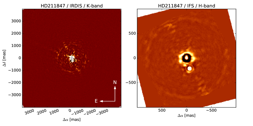
Figure 2: IRDIS imaged processed by Angular Differential Imaging (left, field of view 11 arcsec) and IFS H reduced image (right, field of view 1.7 arcsec) of HD211847. North is up and East is left.

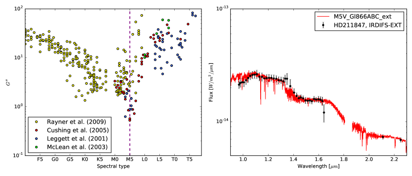
Figure 3: (Left) Goodness-of-fit ($G^{\prime\prime}$ factor, see text for details) with respect to the spectral type for the comparison of our IRDIFS data of the HD 211847 candidate to spectral templates from various stellar and brown-dwarfs libraries; the best fit is shown by a vertical line. (Right) The best-fit spectrum of Gl 866 (plain red line) compared to the extracted data points (black dots).

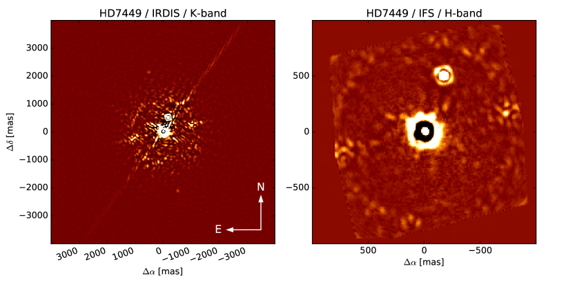
Figure 4: IRDIS image processed by Angular Differential Imaging (left, field of view 11 arcsec) and IFS H image (right, field of view 1.7 arcsec) of HD7449.

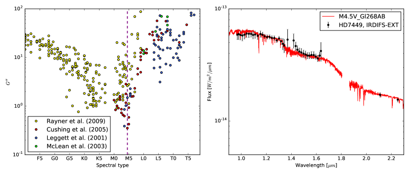
Figure 5: (Left) Goodness-of-fit ($G^{\prime\prime}$ factor, see text for details) with respect to the spectral type for the comparison of our IRDIFS data of the HD 7449 candidate to spectral templates from various stellar and brown-dwarf libraries; the best fit is shown by a vertical line. (Right) The best-fit spectrum of Gl 268 (plain red line) compared to the extracted data points (black dots).

4.1.2 HD7449

Table 6: Astrometric values for HD 7449 B using IRDIS and IFS.

	$\Delta\alpha$ (mas)	$\Delta$Dec (mas)	Separation (mas)	Position Angle (∘)
IRDIS (K1)	-171	505	533	341.3
IRDIS (K2)	-170	508	536	341.5
IFS	-163	499	525	341.9

Table 7: Photometric values for HD 7449 B using IRDIS and IFS and corresponding values in mass.

	Y	J	H	K1	K2
Absolute magnitude	9.49	9.02	8.43	8.10	7.95
Mass (MJup)	176.7	176.0	177.8	188.7	187.7

A candidate companion is detected both with IRDIS and IFS, as shown in Figure 4. It lies at 531$\pm$6 mas from the primary, with a magnitude contrast of 5.

Its astrometric values with respect to HD 7449 are reported in Table 6. The angular separation corresponds to a projected distance of 20.4au. In Table 7, we report the absolute magnitudes derived for HD 7449 B in five different spectral bands. Values for band Y, J, and H are derived from IFS data making a median on the contrast obtained for all the spectral channels in the wavelength range corresponding to that band. Values for K1 and K2 bands are derived from IRDIS data. Using the BT-Settl models and assuming an age of 2 Gyr, we were able to derive the mass of the companions, which are reported in the second row of Table 7.

Our values for HD 7449 B are in good agreement with those reported in Rodigas et al. (2016). The relative position in right ascension and declination also agrees with the expected proper motion of the primary (Fig. 3 in Rodigas et al. (2016)).

We thus infer that the outer radial-velocity companion detected by Dumusque et al. (2011) around HD 7449 and later re-analyzed in Rodigas et al. (2016) is seen in SPHERE images and is a low-mass star with a mass of $0.173\pm 0.006$ M_⊙. The inner planet HD 7449 Ab has a minimum mass of 1.09${}_{-0.19}^{+0.52}$ M_Jup  and period of 1200${}_{-12}^{+16}$ days, eccentricity of 0.8 and semi-major axis of 2.33${}_{-0.02}^{+0.01}$ (Rodigas et al., 2016). If the measured angular separation was the semi-major axis of HD 7449 B, the ratio of semi-major axis would be approximately 9. However, the orbit of the stellar companion is not yet constrained and this ratio could be anywhere in the range 2-20.

As for HD 211847 B, we derived a spectrum of HD 7449 B using both IRDIS and IFS data and compared it to the same template spectra. The final result from this procedure is shown in Figure 5 where the HD 7449 B spectrum is compared to the best fit spectrum from the adopted sample, the M4.5 star Gl268.

4.2 Wide-separation sources

With a larger field of view, IRDIS images contain more detected sources than IFS. For the sake of completeness, we have identified and measured all sources definitely detected in the IRDIS images. The list of these sources is given in Table 8. The angular separation measured for these sources has been translated into physical distance in the case where the source would be at the distance of the primary. This is most likely not the case but allows for identification of possible candidates of interest for dynamical studies, stellar companions at less than $\sim$50au being more susceptible to having a dynamical impact. Apart from HD 211847 and HD 7449, there are no further systems at less than 50au.

The probability of contamination by distant background stars was evaluated with the Besancon Galaxy Model (Robin et al., 2003) and Trilegal (Girardi, 2016). Even for the most crowded fields (around HD 108147 or HD 148156), the star counts in the typical distance and magnitude range of these sources is of the order of 1.5 to 3%. With such a narrow range of probabilities, these stellar counts are thus not very useful for identifying whether such sources are likely due to local environment of the primary target or distant contaminants. Checking the galactic coordinates, we found that almost all targets with companion candidates had galactic latitudes in the range [-20^∘,+20^∘] and their fields at wider angles are also very crowded. There are five exceptions: GJ 3021, HD 28254, HD 7449, HD 211847, and HD 96167. The companion candidates of the first four systems are actually gravitationally bound secondary stars, identified either from previous work (see Table 3) or from this work (see Section 4.1). HD 96167 has a galactic latitude of 44^∘ and its wide field is not crowded. If bound, its companion would have an absolute magnitude of 20.3 in the K band, which corresponds to a 30M_Jup object at an age of 3.8 Gy (Allard, 2014). Follow-up observations could confirm whether this source is a wide brown dwarf companion of HD 96167 or a background star. In the following, we do not consider it as a companion of relevance for binarity frequency.

In addition, we checked the absolute magnitude and corresponding mass of all companion candidates in Table 8, where these sources are at the same distance as the primary star, and found no mass in the range of stellar companions. When no age had been estimated, we assumed an arbitrary age of 4 Gy. For all except the companions flagged as ”confirmed” in Table 8, the detected sources are considered background sources.

Table 8: Companion candidates found in IRDIS images: position angle, separation from the primary star, corresponding distance in au (in those cases where the source is at the distance of the primary target from the Sun), and magnitude difference in the K band. The top lines correspond to the eccentric sample, the middle lines to the comparison sample, and the last line to the intermediate.

Star	Pos. Ang.	Separation	Distance	$\Delta$K	Comment
	degrees	arcsec	au
GJ3021	353	3.97	110.7	5.8	confirmed, see Table 1
HD7449	325	0.25	9.62	4.90	confirmed, see Table 8
HD28254	260	4.89	274.7	$>$ 4.0	confirmed, see Table 1
HD96167	308	3.43	289.6	11.70	to be followed-up
HD108147	3	4.90	189.0	10.90	likely background
HD108147	31	3.59	138.5	12.60	likely background
HD108147	147	4.84	186.7	12.20	likely background
HD108147	289	2.75	106.3	11.85	likely background
HD108147	305	3.46	133.6	12.70	likely background
HD108147	92	3.12	120.9	12.10	likely background
HD108147	41	3.12	120.7	11.40	likely background
HD129445	318	3.25	220.1	9.25	likely background
HD129445	185	3.48	237.6	10.7	likely background
HD129445	247	1.93	131.3	11.00	likely background
HD134060	204	4.25	103.2	10.80	likely background
HD134060	278	2.58	62.5	11.80	likely background
HD134060	288	3.48	84.6	11.60	likely background
HD142415	329	1.58	54.0	10.80	likely background
HD142415	317	4.76	161.9	9.95	likely background
HD148156	121	3.25	173.0	9.40	likely background
HD148156	123	2.56	135.8	9.70	likely background
HD148156	245	5.06	269.2	9.90	likely background
HD148156	113	2.41	128.0	10.60	likely background
HD148156	146	3.81	202.1	10.95	likely background
HD148156	155	1.94	102.9	11.30	likely background
HD148156	7	2.85	151.2	11.30	likely background
HD148156	345	2.45	130.0	11.00	likely background
HD148156	330	2.47	131.0	11.20	likely background
HD148156	320	3.57	189.4	11.50	likely background
HD148156	250	2.10	111.4	11.40	likely background
HD154672	191	4.57	302.3	10.40	likely background
HD157172	14	2.82	89.9	10.10	likely background
HD157172	241	4.26	136.3	12.80	likely background
HD157172	177	5.02	160.1	10.95	likely background
HD211847	194	0.22	11.2	4.80	confirmed, see Table 6
HD60532	181	3.60	92.6	13.50	likely background
HD73256	48	6.17	225.2	9.50	likely background
HD73256	311	6.09	222.	11.80	likely background
HD76700	209	4.96	296.7	9.20	likely background
HD85390	352	4.77	162.1	10.75	likely background
HD85390	37	5.41	184.2	12.50	likely background
HD121504	194	4.50	199.7	6.50	likely background
HD121504	350	3.94	174.8	10.95	likely background
HD121504	80	3.15	139.8	11.35	likely background
HD159868	328	4.77	251.9	12.20	likely background
HD159868	222	3.62	390.8	12.90	likely background
HD159868	145	5.93	312.5	11.75	likely background
HD159868	128	6.52	343.6	10.90	likely background
HD168443	95	2.24	83.7	11.4	likely background
HD168443	214	2.11	78.9	11.95	likely background
HD168443	269	1.15	42.9	9.80	likely background

4.3 Contrast plots

Finally, we present here all detection plots obtained with both instruments, and translate them into detection limits for stellar, or substellar companions.

The contrast plots were derived on all IRDIS ADI-processed images by measuring the azimutally averaged standard deviation with respect to angular separation. A detection limit of 5-$\sigma$ is considered. Each plot is presented in Fig. 6 (top), and the median of the whole sample per bin of angular separation is displayed in Table 11. We get a mean magnitude difference of 10 magnitudes at 0.5 arcsec, with a scatter of 1 magnitude along the sample. This corresponds to a contrast range of $\sim 2.5\times 10^{-3}$ to $\sim 4\times 10^{-5}$, at 5-$\sigma$.

The IFS contrast was calculated for each object in the sample following the same procedure described in Mesa et al. (2015). The contrast plots obtained for each target are shown in Fig. 6 (bottom) with thin lines. The obtained contrasts range from very good ($\sim 10^{-6}$ at a separation of 0.5 arcsec) to very poor ($\sim 10^{-3}$ at the same separation). The median contrast calculated over the whole sample is shown as a thick black line in Fig. 6 (bottom) and Table 11, with a typical value of $\sim 1.25\times 10^{-5}$ at 0.5 arcsec.

This 5-$\sigma$ detection limit is then translated into minimum mass with the aid of BT-Settl stellar models (Allard, 2014), and angular separations are converted into physical separations using the system’s distance given in Table 1 and 2. Figure 7 summarizes the detection limits for the full sample, which are also given at a few specific separations in Tables 9 and 10.

The two stars for which the detection limit is very shallow (Figure 7 bottom) are 91Aqr and HIP 105854, two nearby giant stars. Their luminosity limits the magnitude of any companion, even at high contrasts. For all other cases, we get upper limits of masses in the range 0.1-0.15 M_⊙  at the inner separations of typically 3 to 8au, and lower than 0.07 M_⊙  beyond 10au.

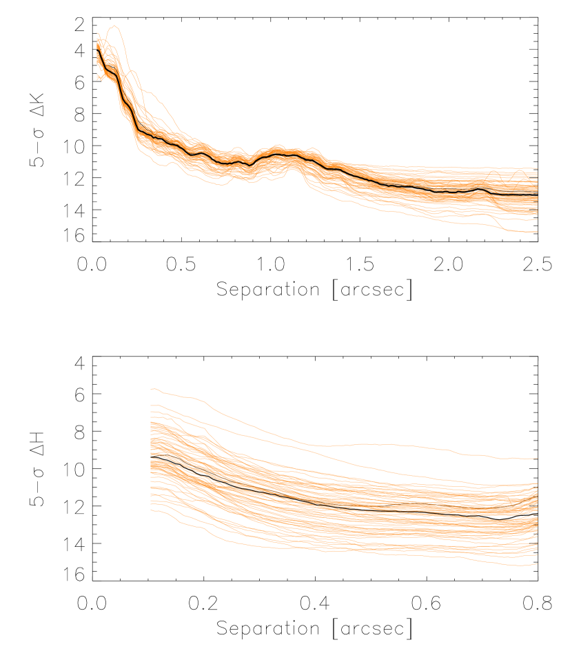
Figure 6: Contrast plots obtained for each single target in the sample (thin lines) with IFS at 1.6 $\mu$m (bottom) and IRDIS at 2.15 $\mu$m (top). The thick black line represents the median contrast obtained over the whole sample. Note the different sizes of the X axis.

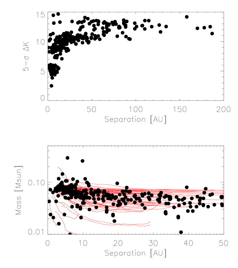
Figure 7: Top: detection limits at 5-$\sigma$ with respect to physical separation, for 0.12-0.24-0.5 and 1” angular separations and all stars included in this study (IRDIS only). Bottom: corresponding minimum mass and physical separation of each star in the sample, derived from IRDIS (black points) and IFS (red lines) detection limits.

5 Discussion and perspectives

We have compared two unbiased samples, one consisting of exoplanet hosts with an eccentric outer planet, and the other made up of exoplanet hosts with circular outer planets. We performed high-contrast imaging on both samples of stars in search for stellar companions, and a posteriori added the information of known visual binaries to have the most complete census of the systems. We also inferred the detection limits for each star, expressed in the mass and physical distance of any putative bound companion. Observations were made using SPHERE on the VLT in 2015 and 2016 with both the IRDIS imager and the IFS spectro-imager.

Although the program was executed as a bad weather filler, much of the data is of good quality and detection limits are consistently better than 10 to 12 magnitudes at 0.5 arcseconds from the primary. For the data cubes where quality was variable, we applied criteria of frame selection before combining the data. A homogeneous treatment was then performed on the 68 data sets, allowing us to draw self-consistent detection analyses. The detection limits drawn from this study, presented in Fig. 7 and Tables 9 and 10, show that stellar companions in the range from a few au to 50au would have been detected, except for two stars that are giant (91 Aqr and HIP 105854). So, combining the already-known stellar companions and the data of this program, we have a global status on the existence of stellar companions in both our samples.

In two systems (HD 7449 and HD 211847), we detected a close-by stellar companion. For HD 7449, we find a secondary separation of $\sim 20.4$au in agreement with Rodigas et al. (2016). This confirms that this system could be one of the most extreme planet-hosting binaries with a ratio between the companion’s and planet’s separations of perhaps less than ten. It may have an architecture similar to that of a small group of other extreme systems, such as $\gamma$ Cephei, HD196885, or HD41004, with a companion at $\sim 20$au and a giant planet around $\sim 2$au, and could present a challenge to the canonical planet formation scenario (Thebault & Haghighipour, 2014). This ratio of semi-major axes should, however, be confirmed by further follow-up of the stellar companion, for which the orbit is not yet fully constrained.

HD 211847 was first identified from its radial-velocity time series, showing the existence of a long-period eccentric companion of $\sim$ 19 M_Jup minimum mass (Sahlmann et al., 2011). The source found in direct imaging is at the correct position to match the radial-velocity companion. This implies that this companion at $\sim$11au is a relatively late M dwarf star with an orbit close to face-on. However, looking back into the radial-velocity time series, it is possible that another short-period signal exists here that requires further data and analysis.

The eccentric sample includes 34 stars (from 35 originally, but HD 211847 may not be an exoplanet host anymore) and 41 (resp., 40) planets. Ten (29%) of the host stars are visual binaries at any separation from 20 to 9200au. In contrast, the comparison circular sample includes 27 stars and 43 exoplanets, and only 3 (11%) visual binaries, at separations ranging from 400 to 1000au. It is striking that more visual binaries are found in the first sample and more exoplanets are present in the second sample. It is not relevant to quantify the significance of this second observation as the exoplanet population in these systems may still be incomplete. Calculating the statistical T-test between both samples for their binary fraction, however, is possible: we get a statistical power of 4.6 while the significance threshold is 1.7; so the null hypothesis of a unique distribution of binaries amongst both samples is excluded. In other words, the proportion of binaries in the eccentric and circular samples are significantly different, despite no other bias than the eccentricity of their outer planet. Also, our detection limits having excluded any other stellar companion in the vicinity of the observed stars, it is striking that the majority of high-eccentricity planets do not orbit stars in multiple systems. The origin of eccentricity in those systems that have a single host star has yet to be explained, possibly involving yet unfound planets. In the case of HD 4113 (part of our eccentric sample), a long-term trend shows the presence of a massive companion that is yet undetected in direct imaging (Tamuz et al., 2008).

Fig.7 indicates that our survey would have detected any potential companion of mass $\geq 0.1M_{\odot}$ with a separation in the 0.05 to 50au range. Interestingly, this range corresponds to where the distribution of binary separation peaks for solar-type stars (Raghavan et al., 2010). Considering the separation distribution given in Fig.13 of that paper, we would expect $\sim 25\%$ of all binaries to fall within that range. Thus, given a binarity rate of approximately $50\%$ (Raghavan et al., 2010), we would expect approximately eight companions in this separation range for the 35+27=62 stars of our combined samples, instead of only one (HD 7449). Our results thus confirm the paucity of planet-host binaries with less than $\sim$50-100au separation found in previous studies. Wang et al. (2014b, a) and Kraus et al. (2016) have reported on such a paucity for a sample of Kepler Objects of Interest, while Eggenberger et al. (2007) has also previously reported a less frequent occurrence of binaries with mean semi-major axes between 35 and 100 au around planet-host stars. Finally, Bonavita & Desidera (2007) also found a lower frequency of planets around binaries with separation smaller than 50-100 au with respect to single stars and members of wide binaries. This first study included a comparison sample of stars for which no radial-velocity companions were detected, while Wang et al. (2014b) and Kraus et al. (2016) based their analysis on a comparison with the binary distribution over the field stars. In our analysis, the comparison is made over the population of known exoplanetary systems with a distinction between dynamically active and inactive systems based on the measured eccentricity of the outer companion. Although our sample is smaller than in those other studies, it is interesting to note that results do not strongly differ and, indeed complement one another.

In addition, there are 12 stars with at least one identified candidate companion in the eccentric sample, and only 6 in the circular sample. This difference is interesting, although most of these candidate companions are very unlikely gravitationally bound to the planetary system, as the dependence with galactic latitude shows. Only HD 96167 might have a low-mass companion, but its identification requires astrometric follow-up observations for confirmation. HD 96167, having an eccentric planet (1.3au, eccentricity 0.71 and minimum mass 0.68 M_Jup), might represent an interesting dynamical architecture, although the outer companion is seen at a large separation of $\sim$ 290au (if it is a bound system).

Appendix A Additional technical details and median contrast

A.1 Observation table

Tables 9 and 10 give the details of the observations presented in this study. Together with the date, mean seeing, and rotation angle obtained for each sequence, the detection limits at various separations are given in the H and K bands.

Table 9: Log of the SPHERE/IRDIFS observations and magnitude contrasts observed at a few specific angular separations.

Name	MJD-OBS	Seeing	Rot	$\Delta$H	$\Delta$H	$\Delta$H	$\Delta$K	$\Delta$K	$\Delta$K	$\Delta$K	$\Delta$K
		arcsec	degrees	0.15”	0.30”	0.60”	0.15”	0.30”	0.60”	1.2”	2.4”
GJ 3021	57305.10	1.25	6.6	9.14	10.87	12.03	6.98	9.50	10.73	11.20	13.53
HD 4113	57303.18	0.85	21.6	12.24	13.74	14.10	7.02	10.14	11.55	11.83	13.27
HD 7449	57304.07	1.00	2.4	7.58	10.18	11.56	6.35	9.06	9.87	10.11	12.06
HD 20782	57309.20	1.23	65.2	8.73	10.89	12.19	6.65	9.10	10.11	10.87	13.15
$\epsilon$ Eridani	57312.19	1.56	11.3	11.24	12.82	14.30	6.77	9.50	10.41	11.60	15.36
HD 28254	57324.29	1.22	4.5	8.97	11.11	12.14	6.49	9.26	10.13	10.82	12.89
HD 30562	57312.24	1.19	4.9	8.40	10.62	12.35	6.62	9.15	10.44	11.06	14.05
HD 33283	57309.30	0.93	6.1	9.81	11.30	12.05	6.93	9.17	9.86	10.82	12.79
HD 39091	57352.22	1.33	6.6	9.21	11.09	12.37	6.23	8.87	10.43	10.68	13.86
HD 43197	57307.34	1.64	23.6	10.08	11.87	12.53	6.60	9.23	10.34	12.01	12.54
HD 44219	57310.30	0.95	3.7	9.98	12.21	13.36	6.81	9.03	10.62	10.83	13.40
HD 66428	57347.30	0.76	7.5	10.04	11.97	12.89	5.99	8.90	10.72	11.38	12.79
HD 86226	57375.33	0.84	0.1	8.36	10.47	11.18	6.54	9.35	10.41	10.38	12.70
HD 86264	57122.06	1.18	19.8	10.64	12.66	13.29	6.75	9.41	11.53	12.08	12.59
HD 96167	57122.09	1.65	12.2	10.77	12.53	13.04	6.26	9.17	11.09	11.72	12.26
HD 98649	57182.96	1.88	3.8	9.20	10.28	11.94	6.91	9.20	10.27	10.96	12.69
HD 106515	57130.11	1.87	7.8	8.95	11.13	12.27	6.72	9.33	10.76	11.45	13.06
HD 108147	57220.99	0.71	4.9	10.04	12.65	13.53	6.60	9.56	10.69	10.92	13.36
HD 129445	57129.26	1.41	7.34	8.22	10.39	11.45	5.58	7.86	10.69	11.04	11.80
HD 142022	57197.16	0.82	2.4	8.50	10.17	11.30	6.28	9.37	10.55	10.94	13.05
HD 142415	57197.20	0.83	4.1	9.63	11.42	12.23	6.70	9.29	10.47	10.99	13.13
HD 148156	57134.37	0.90	4.94	10.34	12.03	12.92	6.58	9.96	11.33	11.34	12.16
HD 154672	57134.39	0.94	5.2	10.22	11.88	12.72	7.05	10.09	11.19	11.37	12.85
HD 157172	57309.01	0.78	0.3	7.85	10.05	11.29	6.80	9.32	10.15	10.57	12.46
HD 168443	57124.40	0.98	15.37	12.68	14.20	14.41	7.75	10.62	12.01	12.25	13.29
HD 181433	57309.03	0.70	7.36	9.53	11.48	12.34	6.46	9.03	10.04	10.75	12.96
HD 187085	57306.01	1.24	34.4	11.46	13.32	14.11	6.68	9.76	11.07	11.63	13.93
HD 196067	57191.40	1.38	3.4	8.92	10.36	12.10	5.86	8.69	10.15	10.89	13.24
HD 210277	57299.10	0.76	14.5	11.46	13.77	14.19	6.74	9.43	11.35	11.80	14.29
HD 211847	57183.39	1.31	6.7	10.37	11.07	12.87	6.69	8.34	10.50	11.08	12.21
HD 215497	57304.05	1.06	9.09	9.82	11.65	12.46	6.71	9.40	10.22	11.12	13.22
HD 217107	57183.37	1.55	3.2	10.48	11.14	12.92	6.94	9.26	10.22	10.68	13.90
HD 219077	57182.39	1.29	3.3	10.37	11.27	12.80	6.89	9.41	10.22	10.87	14.08
HD 222582	57193.41	1.07	5.3	9.40	10.9	11.57	4.60	7.90	9.87	10.75	12.48

Table 10: Log of the SPHERE/IRDIFS observations and magnitude contrasts observed at a few specific angular separations (cont’d).

Name	MJD-OBS	Seeing	Rot	$\Delta$H	$\Delta$H	$\Delta$H	$\Delta$K	$\Delta$K	$\Delta$K	$\Delta$K	$\Delta$K
		arcsec	degrees	0.15”	0.30”	0.60”	0.15”	0.30”	0.60”	1.2”	2.4”
HD 1461	57299.13	0.73	10.8	10.19	12.65	13.38	6.13	9.05	10.88	11.73	14.16
HD 4208	57308.08	0.82	2.3	9.27	10.85	12.39	6.77	9.71	10.64	10.76	13.47
HD 10180	57300.09	0.83	8.0	10.19	12.83	13.48	6.32	9.34	10.41	11.07	13.66
HD 11964	57306.12	1.05	2.13	8.68	10.32	11.91	6.89	9.17	10.63	10.72	13.45
HD 20794	57309.22	1.43	22.8	11.93	13.34	14.70	6.55	9.16	10.88	12.43	15.37
HD 23079	57312.17	1.48	7.8	9.93	11.62	12.34	6.88	9.44	10.26	11.07	13.41
HD 38801	57312.26	1.27	50.0	9.90	11.37	12.06	6.69	9.43	10.36	11.03	12.47
BD-061339	57309.36	1.16	6.1	9.40	11.09	11.91	5.81	8.92	9.94	10.93	12.73
HD 47186	57343.29	1.17	5.5	10.13	11.87	12.75	6.28	9.37	10.87	10.83	13.04
HD 60532	57343.30	1.40	2.2	7.28	9.96	11.60	6.31	9.15	10.46	10.50	14.03
HD 65216	57350.34	1.01	8.9	9.74	11.26	11.97	5.29	8.37	10.08	10.73	12.01
HD 73256	57378.36	0.77	53.78	10.93	12.72	13.26	6.63	9.40	10.90	11.36	13.31
HD 75289	57395.17	0.67	2.8	10.23	12.28	13.63	6.23	8.75	10.47	10.48	13.39
HD 76700	57347.35	0.90	2.9	8.12	10.13	11.36	6.28	8.89	10.58	10.67	12.60
HD 82943	57122.04	1.21	16.7	11.77	13.43	13.61	7.27	9.45	11.31	11.68	12.26
HD 83443	57377.25	0.40	2.49	10.17	11.32	12.49	6.50	9.30	10.66	10.24	12.58
HD 85390	57343.33	2.10	7.2	6.98	8.49	10.49	4.99	8.19	9.95	10.62	11.93
HD 86081	57347.33	0.78	1.2	8.24	9.96	10.88	6.42	9.17	10.46	10.37	11.43
HD 92788	57183.98	1.80	2.5	7.90	9.60	11.24	6.61	9.25	9.82	10.53	13.18
HD 104067	57138.07	1.84	5.4	10.38	11.84	12.96	6.68	9.88	10.88	11.34	13.57
HD 109749	57221.02	0.66	1.9	8.05	10.57	11.42	6.84	9.49	10.57	10.79	11.56
HD 117618	57197.18	0.78	2.0	9.20	10.78	11.83	6.90	9.40	10.49	11.01	13.17
HD 121504	57270.99	0.72	3.85	9.09	10.62	11.53	6.20	9.18	10.39	10.79	12.97
HD 134060	57140.39	0.90	2.6	9.46	11.62	12.34	6.07	9.69	10.75	11.20	13.15
HD 150433	57135.36	1.06	3.8	8.99	11.22	12.45	6.62	10.15	10.83	11.05	13.53
HD 159868	57133.39	1.05	5.4	9.68	11.17	12.71	5.91	8.92	10.76	11.18	13.71
HD 192263	57301.05	1.08	7.5	9.98	12.00	13.22	6.89	9.50	9.94	10.77	12.64
HIP 105854	57182.37	1.30	8.9	11.56	12.93	14.28	6.87	9.51	10.42	11.34	14.61
HD 212301	57182.41	-	2.56	8.18	9.59	10.99	6.99	9.72	10.87	11.01	11.86
91 Aqr	57183.41	1.39	8.8	9.80	11.17	11.90	6.75	9.05	10.19	10.55	14.28

A.2 Frame selection

We used the following method to select the frames:

• First, we estimated the difference image between each frame and the cube median; referred to as the residual frame in the following.

• We measure three quantities in the residual frames: i) the maximum of the peak in the central area, ii) the flux at the location of the residual diffraction of the spiders, and iii) the average flux in the darkest, AO-corrected part of the image, above and below the peak. Each quantity is normalized by the median of the time sequence, for each cube.

• We plotted the time evolution of these quantities for each cube and determined threshold for each, beyond which the data should be removed. This trade-off analysis aims at keeping the maximum number of frames while not increasing the noise in the combined image. It is usually quite clear from the data where the line should be drawn, as illustrated in some of the examples shown in Fig. 8.

• We removed all frames when either the normalized peak was lower than 0.5, the normalized spider flux was more than 2.0, or the normalized dark flux was more than 2.0. These values turned out to be a suitable compromise for all data cubes.

The number of removed frames for each observation is given in Tables 9 and 10 for reference. Not many sequences are affected by frame selection, an indication that this filler program was used in reasonably good conditions in most cases. For some data cubes, however, the frame selection removed more than half of the data.

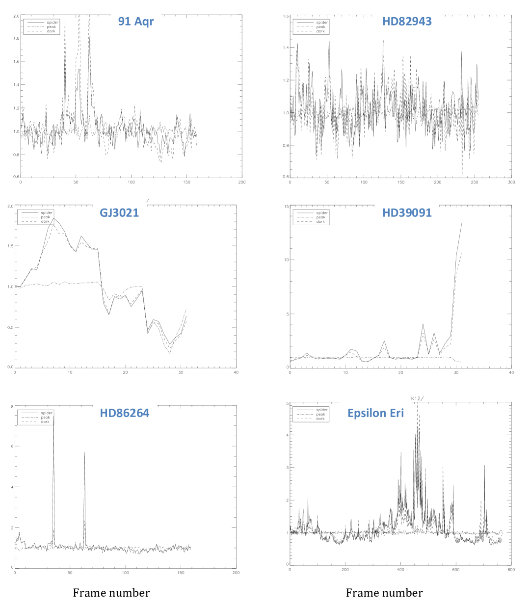
Figure 8: Examples of flux criteria in various places of the image along the IRDIS data cubes used for the selection of valid frames in the combination processing (see text). The plain line shows the flux in the image close to the spider (indicating a pupil misalignment), the dashed line shows the flux in the darkest region of the image, and the dot-dash line shows the peak flux in the center of the target.

A.3 Median detection limit

The contrast plots as a function of separation obtained in this analysis are very similar for all objects, with offsets due to the data quality and/or the star magnitude. Table 11 gives the median contrast plot in H and K magnitudes, obtained respectively from IFS-YH and IRDIS-K12 configurations. These values correspond to the thick black curves shown on Figure 6.

Table 11: Median contrast curve as a function of angular separation in YH from IFS data, and in K from IRDIS data. These curves are calculated from the 64 data sets analyzed in this article, and shown on Figure 6.

Sep	$\Delta$H	$\Delta$K
arcsec	mag	mag
0.10	9.39	5.39
0.15	9.75	6.21
0.20	10.37	7.50
0.25	10.91	8.84
0.30	11.26	9.25
0.35	11.55	9.49
0.40	11.92	9.67
0.45	12.11	9.93
0.50	12.24	10.17
0.55	12.30	10.59
0.60	12.35	10.49
0.65	12.47	10.65
0.70	12.57	11.02
0.75	12.64	11.13
0.80	12.41	11.05
0.90	-	11.15
1.00	-	10.62
1.10	-	10.63
1.20	-	10.88
1.30	-	11.36
1.40	-	11.57
1.50	-	12.00
1.60	-	12.33
1.70	-	12.54
1.80	-	12.59
1.90	-	12.82
2.00	-	12.91
2.10	-	12.87
2.20	-	12.78
2.30	-	13.07
2.40	-	13.07
2.50	-	13.08