Demand-Driven Pointer Analysis with Strong Updates via Value-Flow Refinement

Abstract

We present a new demand-driven flow- and context-sensitive pointer analysis with strong updates for C programs, called Supa, that enables computing points-to information via value-flow refinement, in environments with small time and memory budgets such as IDEs. We formulate Supa by solving a graph-reachability problem on an inter-procedural value-flow graph representing a program’s def-use chains, which are pre-computed efficiently but over-approximately. To answer a client query (a request for a variable’s points-to set), Supa reasons about the flow of values along the pre-computed def-use chains sparsely (rather than across all program points), by performing only the work necessary for the query (rather than analyzing the whole program). In particular, strong updates are performed to filter out spurious def-use chains through value-flow refinement as long as the total budget is not exhausted. Supa facilitates efficiency and precision tradeoffs by applying different pointer analyses in a hybrid multi-stage analysis framework.

We have implemented Supa in LLVM (3.5.0) and evaluate it by choosing uninitialized pointer detection as a major client on 18 open-source C programs. As the analysis budget increases, Supa achieves improved precision, with its single-stage flow-sensitive analysis reaching 97.4% of that achieved by whole-program flow-sensitive analysis by consuming about 0.18 seconds and 65KB of memory per query, on average (with a budget of at most 10000 value-flow edges per query). With context-sensitivity also considered, Supa’s two-stage analysis becomes more precise for some programs but also incurs more analysis times. Supa is also amenable to parallelization. A parallel implementation of its single-stage flow-sensitive analysis achieves a speedup of up to 6.9x with an average of 3.05x a 8-core machine with respect its sequential version.

¡ccs2012¿ ¡concept¿ ¡concept_id¿10011007.10011006.10011041¡/concept_id¿ ¡concept_desc¿Software and its engineering Software verification and validation¡/concept_desc¿ ¡concept_significance¿500¡/concept_significance¿ ¡/concept¿ ¡concept¿ ¡concept_id¿10011007.10011074.10011099.10011102¡/concept_id¿ ¡concept_desc¿Software and its engineering Software defect analysis¡/concept_desc¿ ¡concept_significance¿100¡/concept_significance¿ ¡/concept¿ ¡concept¿ ¡concept_id¿10003752.10003753.10003761¡/concept_id¿ ¡concept_desc¿Theory of computation Program reasoning¡/concept_desc¿ ¡concept_significance¿100¡/concept_significance¿ ¡/concept¿ ¡/ccs2012¿

[100]Software and its engineering Software verification and validation [100]Software and its engineering Software defect analysis [100]Theory of computation Program analysis

1 INTRODUCTION

Pointer analysis is one of the most fundamental static program analyses, on which virtually all others are built. The goal of pointer analysis is to compute an approximation of the set of abstract objects that a pointer can refer to. A pointer analysis is (1) flow-sensitive if it respects control flow and flow-insensitive otherwise and (2) context-sensitive if it distinguishes different calling contexts and context-insensitive otherwise.

Strong updates, where stores overwrite, i.e., kill the previous contents of their abstract destination objects with new values, is an important factor in the precision of pointer analysis [16, 25]. In the case of weak updates, these objects are assumed conservatively to also retain their old contents. Strong updates are possible only if flow-sensitivity is maintained. In addition, a flow-sensitive analysis can strongly update an abstract object written at a store if and only if that object has exactly one concrete memory address, known as a singleton. By applying strong updates where needed, a pointer analysis can improve precision, thereby providing significant benefits to many clients, such as change impact analysis [1], bug detection [61, 60], security analysis [4], type state verification [14], compiler optimization [49, 48, 53], and symbolic execution [6].

In this paper, we introduce a demand-driven pointer analysis for C by investigating how to perform strong updates effectively in a flow- and context-sensitive framework. For C programs, flow-sensitivity is important in achieving the precision required by the afore-mentioned client applications due to strong updates performed. If context-sensitivity is also considered, some more strong updates are possible for some programs at the expense of more analysis times. For object-oriented languages like Java, context-sensitivity (without strong updates) is widely used in achieving useful precision [26, 28, 31, 32, 41, 54, 58].

Ideally, strong updates at stores should be performed by analyzing all paths independently by solving a meet-over-all-paths (MOP) problem. However, even with branch conditions being ignored, this problem is intractable due to potentially unbounded number of paths that must be analyzed [23, 37].

Instead, traditional flow-sensitive pointer analysis (FS) for C [19, 21] computes the maximal-fixed-point solution (MFP) as an over-approximation of MOP by solving an iterative data-flow problem. Thus, the data-flow facts that reach a confluence point along different paths are merged. Improving on this, sparse flow-sensitive pointer analysis (SFS) [27, 17, 35, 62, 63] boosts the performance of FS in analyzing large C programs while maintaining the same strong updates done by FS. The basic idea is to first conduct a pre-analysis on the program to over-approximate its def-use chains and then perform FS by propagating the data-flow facts, i.e., points-to information sparsely along only the pre-computed def-use chains (aka value-flows) instead of all program points in the program’s control-flow graph (CFG).

Recently, an approach [25] for performing strong updates in C programs is introduced. It sacrifices the precision of FS to gain efficiency by applying strong updates at stores where flow-sensitive singleton points-to sets are available but falls back to the flow-insensitive points-to information otherwise.

By nature, the challenge of pointer analysis is to make judicious tradeoffs between efficiency and precision. Virtually all of the prior analyses for C that consider some degree of flow-sensitivity are whole-program analyses. Precise ones are unscalable since they must typically consider both flow- and context-sensitivity (FSCS) in order to maximize the number of strong updates performed. In contrast, faster ones like [25] are less precise, due to both missing strong updates and propagating the points-to information flow-insensitively across the weakly-updated locations.

In practice, a client application of a pointer analysis may require only parts of the program to be analyzed. In addition, some points-to queries may demand precise answers while others can be answered as precisely as possible with small time and memory budgets. In all these cases, performing strong updates blindly across the entire program is cost-ineffective in achieving precision.

 

Figure 1: Overview of Supa

For C programs, how do we develop precise and efficient pointer analyses that are focused and partial, paying closer attention to the parts of the programs relevant to on-demand queries? Demand-driven analyses for C [18, 64, 67] and Java [29, 40, 43, 46, 59] are flow-insensitive and thus cannot perform strong updates to produce the precision needed by some clients. Boomerang [42] represents a recent flow- and context-sensitive demand-driven pointer analysis for Java. However, its access-path-based approach performs strong updates at a store $a.f=\dots$ only partially, by updating $a.f$ strongly and the aliases of $a.f.*$ weakly. Elsewhere, advances in whole-program flow-sensitive analysis for C have exploited some form of sparsity to improve performance [17, 27, 35, 62, 63]. However, how to replicate this success for demand-driven flow-sensitive analysis for C is unclear. Finally, it remains open as to whether sparse strong update analysis can be performed both flow- and context-sensitively on-demand to avoid under- or over-analyzing.

In this paper, we introduce Supa, the first demand-driven pointer analysis with strong updates for C, designed to support flexible yet effective tradeoffs between efficiency and precision in answering client queries, in environments with small time and memory budgets such as IDEs. As shown in Figure 1, the novelty behind Supa lies in performing Strong UPdate Analysis precisely by refining imprecisely pre-computed value-flows away in a hybrid multi-stage analysis framework. Given a points-to query, strong updates are performed by solving a graph-reachability problem on an inter-procedural value-flow graph that captures the def-use chains of the program obtained conservatively by a pre-analysis. Such over-approximated value-flows can be obtained by applying Andersen’s analysis [3] (flow- and context-insensitively). Supa conducts its reachability analysis on-demand sparsely along only the pre-computed value-flows rather than control-flows. In addition, Supa filters out imprecise value-flows by performing strong updates flow- and context-sensitively where needed with no loss of precision as long as the total analysis budget is sufficient. The precision of Supa depends on the degree of value-flow refinement performed under a budget. The more spurious value-flows Supa removes, the more precise the points-to facts are.

Supa handles large C programs by staging analyses in increasing efficiency but decreasing precision in a hybrid manner. Currently, Supa proceeds in two stages by applying FSCS and FS in that order with a configurable budget for each analysis. When failing to answer a query in a stage within its alloted budget, Supa downgrades itself to a more scalable but less precise analysis in the next stage and will eventually fall back to the pre-computed flow-insensitive information. At each stage, Supa will re-answer the query by reusing the points-to information found from processing the current and earlier queries. By increasing the budgets used in the earlier stages (e.g., FSCS), Supa will obtain improved precision via improved value-flow refinement.

In summary, this paper makes the following contributions:

• We present the first demand-driven flow- and context-sensitive pointer analysis with strong updates for C that enables computing precise points-to information by refining away imprecisely precomputed value-flows, subject to analysis budgets.

• We introduce a hybrid multi-stage analysis framework that facilitates efficiency and precision tradeoffs by staging different analyses in answering client queries.

• We have produced an implementation of Supa in LLVM (3.5.0) [55]. We evaluate Supa with uninitialized pointer detection as a practical client by using a total of 18 open-source C programs. As the analysis budget increases, Supa achieves improved precision, with its single-stage flow-sensitive analysis reaching 97.4% of that achieved by whole-program flow-sensitive analysis, by consuming about 0.18 seconds and 65KB of memory per query, on average (with a per-query budget of at most 10000 value-flow edges traversed). With context-sensitivity also being considered, more strong updates are also possible. Supa’s two-stage analysis then becomes more precise for some programs at the expense of more analysis times.

• We present four case studies to demonstrate that Supa is effective in checking whether variables are initialized or not in real-world applications.

• We show that Supa is amenable to parallelization. To demonstrate this, we have developed a parallel implementation of Supa’s single-stage flow-sensitive analysis based on Intel Threading Building Blocks (TBB), achieving a speedup of up to 6.9x with an average of 3.05x a 8-core machine over its sequential version.

The rest of this paper is organized as follows. Section 2 provides the background information. Section 3 presents a motivating example. Section 4 introduces our formalism for Supa. Section 5 discusses and analyzes our experimental results. Section 6 contains four case studies. Section 7 describes a parallel implementation of Supa. Section 8 describes the related work. Finally, Section 9 concludes the paper.

2 Background

We describe how to represent a C program by an interprocedural sparse value-flow graph to enable demand-driven pointer analysis via value-flow refinement. Section 2.1 introduces the part of LLVM-IR relevant to pointer analysis. Section 2.2 describes how to put top-level variables in SSA form. Section 2.3 describes how to put address-taken variables in SSA form. Section 2.4 constructs a sparse value-flow graph that represents the def-use chains for both top-level and address-taken variables in the program.

2.1 LLVM-IR

We perform pointer analysis in the LLVM-IR of a program, as in [17, 25, 27, 51, 62, 5]. The domains and the LLVM instructions relevant to pointer analysis are given in Table 1. The set of all variables $\mathcal{V}$ are separated into two subsets, $\mathcal{O}$ that contains all possible abstract objects, i.e., address-taken variables of a pointer and $\mathcal{P}$ that contains all top-level variables.

In LLVM-IR, top-level variables in $\mathcal{P}=\mathcal{S}\cup\mathcal{G}$, including stack virtual registers (symbols starting with ”%”) and global variables (symbols starting with ”@”) are explicit, i.e., directly accessed. Address-taken variables in $\mathcal{O}$ are implicit, i.e., accessed indirectly at LLVM’s load or store instructions via top-level variables.

Only a subset of the complete LLVM instruction set that is relevant to pointer analysis are modeled. As in Table 1, every function $f$ of a program contains nine types of instructions (statements), including seven types of instructions used in the function body of $f$, and one FunEntry instruction $f(r_{1},\dots,r_{n})$ with the declarations of the parameters of $f$, and one FunExit instruction $ret_{f}\ p$ as the unique return of $f$. Note that the LLVM pass UnifyFunctionExitNodes is executed before pointer analysis in order to ensure that every function has only one FunExit instruction.

Table 1: Domains and LLVM instructions used by pointer analysis.

Analysis Domains

LLVM Instruction Set

$\ell$ $\in$ $\mathcal{L}$ instruction labels $fld$ $\in$ $\mathcal{C}$ constants (field accesses) $s$ $\in$ $\mathcal{S}$ stack virtual registers $g$ $\in$ $\mathcal{G}$ global variables $f$ $\in$ $\mathcal{F}\subseteq\mathcal{G}$ program functions $p,q,r,x,y$ $\in$ $\mathcal{P}=\mathcal{S}\cup\mathcal{G}$ top-level variables $o,a,b,c,d$ $\in$ $\mathcal{O}$ address-taken variables $v$ $\in$ $\mathcal{V}=\mathcal{P}\cup\mathcal{O}$ program variables

AddrOf $p$ = $\ \&o$ Copy $p$ = $\ q$ Phi $p$ = $\phi(q,r)$ Field $p$ = $\ \&q\!\rightarrow\!fld$ Load $p$ = $\ *q$ Store $*p$ = $\ q$ Call $p$ = $\ q(r_{1},\dots,r_{n})$ FunEntry $f(r_{1},\dots,r_{n})$ FunExit $ret_{f}\ p$

Let us go through the seven types of instructions used inside a function. For an AddrOf instruction $p\!\!=\!\!\&o$, known as an allocation site, $o$ is one of the following objects: (1) a stack object, $o_{\ell}$, where $\ell$ is its allocation site (via an LLVM alloca instruction), (2) a global object, i.e., a global object $o_{\ell}$, where $\ell$ is its allocation site or a program function $o_{f}$, where $f$ is its name, and (3) a dynamically created heap object $o^{h}_{\ell}$, where $\ell$ is its heap allocation site (e.g., via a malloc() call). For each object $o$ (except for a function), we write $o_{fld}$ to represent the sub-object that corresponds to its field $fld$. For flow-sensitive pointer analysis, the initializations for global objects take place at the entry of main().

Copy denotes a casting instruction (e.g., bitcast) in LLVM. Phi is a standard SSA instruction introduced at a confluence point in the CFG to select the value of a variable from different control-flow branches. Load (Store) is a memory accessing instruction that reads (write) a value from (into) an address-taken object.

Our handling of field-sensitivity is ANSI-compliant. Given a pointer to an aggregate (e.g., a struct or an array), pointer arithmetic used for accessing anything other than the aggregate itself has undefined behavior [36, 20] and thus not modeled. To model the field accesses of a struct object, Field represents a getelementptr instruction with its field offset $fld$ as a constant value. A getelementptr instruction that operates on a non-constant field of a struct is modeled as Copy instructions, one for every field of the struct conservatively. Arrays are treated monolithically.

Call, $p=q(r_{1},\dots,r_{n})$, denotes a call instruction, where $q$ can be either a global variable (for a direct call) or a stack virtual register (for an indirect call).

2.2 SSA Form for Top-Level Variables

LLVM-IR is known as a partial SSA form since only top-level variables are in SSA form. In LLVM-IR, top-level variables are explicit, i.e., directly accessed and can thus be put in SSA form by using a standard SSA construction algorithm [10] (with Phi instructions inserted at confluence points).

Figure 2: A swap example and its partial SSA form.

Let us illustrate LLVM’s partial SSA form by using an example in Figure 2. Figure 2(a) shows a swap program in C and Figure 2(b) gives its corresponding partial SSA form. Figures 2(c) and (d) depict some (runtime) points-to relations before and after the swap operation. In this example, we have $p,q,x,y,t1,t2\in\mathcal{P}$ and $a,b,c,d\in\mathcal{O}$. Note that $x,y,t1$ and $t2$ are new temporary registers introduced in order to put the program given in Figure 2(a) into the partial SSA form given in Figure 2(b). In particular, $*p=*q$ is decomposed into $t2=*q$ and $*p=t2$, where $t2$ is a top-level pointer.

In LLVM-IR, all top-level variables are in SSA form. In this example, all top-level variables are trivially in SSA form, as each has exactly one definition only. As a result, the def-use chains for top-level variables are readily available.

However, address-taken variables are accessed indirectly at loads and stores via top-level variables and thus not in SSA form. For example, the address-taken variable $a$ is defined implicitly twice, once at $*p=x$ and once at $*p=t2$, and the address-taken variable $c$ is also defined implicitly twice, once at $*q=y$ and once at $*q=t1$. As a result, the def-use chains for address-taken variables are not immediately available.

2.3 SSA Form for Address-Taken Variables

Starting with LLVM’s partial SSA form, we first perform a pre-analysis by using Andersen’s algorithm flow- and context-insensitively [3], implemented in SVF [50]. We then put address-taken variables in memory SSA form, by using the SSA construction algorithm [10]. Imprecise points-to information computed this way will be refined by our demand-driven pointer analysis.

Given a variable $v$, $\emph{AnderPts}(v)$ represents its points-to set computed by Andersen’s algorithm. There are two steps  [52], illustrated in Figures 3(a) and (b) intraprocedurally and in Figures 4(a) and (b) interprocedurally.

Step 1: Computing Modification and Reference Side-Effects

As shown in Figure 3(a), every load, e.g., $t1=*q$ is annotated with a ${\color[rgb]{0.00,0.47,0.00}{\color[rgb]{0.00,0.47,0.00}\bm{\mu}}(a)}$ operator for each object $a$ pointed by $q$, i.e., $a\in\emph{AnderPts}(q)$ to represent a potential use of $a$ at the load. Similarly, every store, e.g., $*p=x$ is annotated with a ${\color[rgb]{0.00,0.47,0.00}a\!=\!{\color[rgb]{0.00,0.47,0.00}\bm{\chi}}(a)}$ operator for each object $a\in\emph{AnderPts}(p)$ to represent a potential def and use of $a$ at the store. If $a$ can be strongly updated, then $a$ receives whatever $x$ points to and the old contents in $a$ are killed. Otherwise, $a$ must also incorporate its old contents, resulting in a weak update to $a$.

Figure 3: Memory SSA form and sparse value-flows constructed intraprocedurally for Figure 2, obtained with Andersen’s analysis: $\emph{AnderPts}(p)=\{a\}$ and $\emph{AnderPts}(q)=\{c\}$.

Figure 4: Memory SSA form and sparse value-flows constructed interprocedurally for an example modified from Figure 2 with its four swap instructions moved into a separate function, called swap. $\ell_{8}$ and $\ell_{13}$ correspond to the FunEntry and FunExit of swap.

We compute the side-effects of a function call by applying a lightweight interprocedural mod-ref analysis [52, §4.2.1]. For a given callsite $\ell$, it is annotated with ${\color[rgb]{0.00,0.47,0.00}{\color[rgb]{0.00,0.47,0.00}\bm{\mu}}(a)}$ (${\color[rgb]{0.00,0.47,0.00}a\!=\!{\color[rgb]{0.00,0.47,0.00}\bm{\chi}}(a)}$) if $a$ may be read (modified) inside the callees of $\ell$ (discovered by Andersen’s pointer analysis). In addition, appropriate ${\color[rgb]{0.00,0.47,0.00}\bm{\chi}}$ and ${\color[rgb]{0.00,0.47,0.00}\bm{\mu}}$ operators are also added for the FunEntry and FunExit instructions of these callees in order to mimic passing parameters and returning results for address-taken variables.

Figure 4(a) gives an example modified from Figure 3(a) by moving the four swap instructions into a function, swap. For read side-effects, ${\color[rgb]{0.00,0.47,0.00}{\color[rgb]{0.00,0.47,0.00}\bm{\mu}}(a)}$ and ${\color[rgb]{0.00,0.47,0.00}{\color[rgb]{0.00,0.47,0.00}\bm{\mu}}(c)}$ are added before callsite $\ell_{7}$ to represent the potential uses of $a$ and $c$ in swap. Correspondingly, swap’s FunEntry instruction $\ell_{8}$ is annotated with ${\color[rgb]{0.00,0.47,0.00}a\!=\!{\color[rgb]{0.00,0.47,0.00}\bm{\chi}}(a)}$ and ${\color[rgb]{0.00,0.47,0.00}c\!=\!{\color[rgb]{0.00,0.47,0.00}\bm{\chi}}(c)}$ to receive the values of $a$ and $c$ passed from $\ell_{7}$. For modification side-effects, ${\color[rgb]{0.00,0.47,0.00}a\!=\!{\color[rgb]{0.00,0.47,0.00}\bm{\chi}}(a)}$ and ${\color[rgb]{0.00,0.47,0.00}c\!=\!{\color[rgb]{0.00,0.47,0.00}\bm{\chi}}(c)}$ are added after $\ell_{7}$ to receive the potentially modified values of $a$ and $c$ returned from swap’s FunExit instruction $\ell_{13}$, which are annotated with ${\color[rgb]{0.00,0.47,0.00}{\color[rgb]{0.00,0.47,0.00}\bm{\mu}}(a)}$ and ${\color[rgb]{0.00,0.47,0.00}{\color[rgb]{0.00,0.47,0.00}\bm{\mu}}(c)}$.

Step 2: Memory SSA Renaming

All the address-taken variables are converted into SSA form as suggested in [9]. Every ${\color[rgb]{0.00,0.47,0.00}{\color[rgb]{0.00,0.47,0.00}\bm{\mu}}(a)}$ is treated as a use of $a$. Every ${\color[rgb]{0.00,0.47,0.00}a\!=\!{\color[rgb]{0.00,0.47,0.00}\bm{\chi}}(a)}$ is treated as both a def and use of $a$, as $a$ may admit only a weak update. Then the SSA form for address-taken variables is obtained by applying a standard SSA construction algorithm [10].

For the program annotated with $\mu$’s and $\chi$’s in Figure 3(a), Figure 3(b) gives its memory SSA form. Similarly, Figure 4(b) gives the memory SSA form for Figure 4(a).

Table 2: Def-use information of both top-level and address-taken variables. $Def_{v}$ ($Use_{v}$) denotes the set of definition (use) instructions for a variable $v\in\mathcal{V}$.

Instruction     $\ell$	Defs and Uses of Variables in Memory SSA Form
$p=\&o$	$\{\ell\}=Def_{p}$
$p=q$	$\{\ell\}=Def_{p}$  $\ell\in Use_{q}$
$p=\phi(q,r)$	$\{\ell\}=Def_{p}$  $\ell\in Use_{q}$  $\ell\in Use_{r}$
$p=\&q\!\rightarrow\!fld$	$\{\ell\}=Def_{p}$  $\ell\in Use_{q}$
$p=*q$           ${\color[rgb]{0.00,0.47,0.00}{\color[rgb]{0.00,0.47,0.00}\bm{\mu}}(a_{i})}$	$\{\ell\}=Def_{p}$  $\ell\in Use_{q}$  $\ell\in Use_{a_{i}}$
$*p=q$           ${\color[rgb]{0.00,0.47,0.00}a_{i+1}\!=\!{\color[rgb]{0.00,0.47,0.00}\bm{\chi}}(a_{i})}$	$\ell\in Use_{p}$  $\ell\in Use_{q}$  $\ell\in Def_{a_{i+1}}$  $\ell\in Use_{a_{i}}$
$p=q(r_{1},\dots,r_{n})$	$\{\ell\}=Def_{p}$  $\ell\in Use_{q}$  $\forall\ i\in 1,\dots,n:\!\ \!\ell\in Use_{r_{i}}$
${\color[rgb]{0.00,0.47,0.00}{\color[rgb]{0.00,0.47,0.00}\bm{\mu}}(a_{i})}$  ${\color[rgb]{0.00,0.47,0.00}a_{j+1}\!=\!{\color[rgb]{0.00,0.47,0.00}\bm{\chi}}(a_{j})}$	$\ell\in Use_{a_{i}}$  $\ell\in Def_{a_{j+1}}$  $\ell\in Use_{a_{j}}$
$f(r_{1},\dots,r_{n})$    ${\color[rgb]{0.00,0.47,0.00}a_{i+1}\!=\!{\color[rgb]{0.00,0.47,0.00}\bm{\chi}}(a_{i})}$	$\forall\ i\in 1,\dots,n:\!\ \!\ell\in Def_{r_{i}}$   $\ell\in Def_{a_{i+1}}$   $\ell\in Use_{a_{i}}$
$ret_{f}\ p$           ${\color[rgb]{0.00,0.47,0.00}{\color[rgb]{0.00,0.47,0.00}\bm{\mu}}(a_{i})}$	$\ell\in Use_{p}$  $\ell\in Use_{a_{i}}$

[INTRA-TOP] $\frac{\begin{array}[c]{c}\begin{tabular}[]{lll}$\ell\in Def_{p}$ \quad$\ell^{\prime}\in Use_{p}$\\ \end{tabular}\end{array}}{\begin{array}[c]{c}\begin{tabular}[]{ll}$\ell\xrightarrow{p}\ell^{\prime}$\\ \end{tabular}\end{array}}$   [INTRA-ADDR] $\frac{\begin{array}[c]{c}\begin{tabular}[]{lll}$\ell\in Def_{a_{i}}$ \quad$\ell^{\prime}\in Use_{a_{i}}$\\ \end{tabular}\end{array}}{\begin{array}[c]{c}\begin{tabular}[]{ll}$\ell\xrightarrow{a}\ell^{\prime}$\\ \end{tabular}\end{array}}$

[INTER-CALL-TOP] $\frac{\begin{array}[c]{c}\begin{tabular}[]{lll}$\ell:p=q(r_{1},\dots,r_{n})$ \quad$o_{f}\in\emph{AnderPts}(q)$ \quad$\ell^{\prime}:f(r^{\prime}_{1},\dots,r^{\prime}_{n})$\\ \end{tabular}\end{array}}{\begin{array}[c]{c}\begin{tabular}[]{ll}$\forall i\in 1,\dots,n:\ell\xrightarrow{r_{i}}\ell^{\prime}$\\ \end{tabular}\end{array}}$

[INTER-RET-TOP] $\frac{\begin{array}[c]{c}\begin{tabular}[]{lll}$\ell:p=q(\dots)$ \quad$a_{f}\in\emph{AnderPts}(q)$ \quad$\ell^{\prime}:ret_{f}\ p^{\prime}$\\ \end{tabular}\end{array}}{\begin{array}[c]{c}\begin{tabular}[]{ll}$\ell^{\prime}\xrightarrow{p}\ell$\\ \end{tabular}\end{array}}$

[INTER-CALL-ADDR] $\frac{\begin{array}[c]{c}\begin{tabular}[]{lll}$\ell:p=q(\dots)$ ${\color[rgb]{0,0,1}{\color[rgb]{0.00,0.47,0.00}{\color[rgb]{0.00,0.47,0.00}\bm{\mu}}(a_{i})}}$ \quad$a_{f}\in\emph{AnderPts}(q)$ \quad$\ell^{\prime}:f(\dots)$ ${\color[rgb]{0,0,1}{\color[rgb]{0.00,0.47,0.00}a_{j+1}\!=\!{\color[rgb]{0.00,0.47,0.00}\bm{\chi}}(a_{j})}}$\\ \end{tabular}\end{array}}{\begin{array}[c]{c}\begin{tabular}[]{ll}$\ell\xrightarrow{a}\ell^{\prime}$\\ \end{tabular}\end{array}}$

[INTER-RET-ADDR] $\frac{\begin{array}[c]{c}\begin{tabular}[]{lll}$\ell:\_=q(\dots)$ ${\color[rgb]{0.00,0.47,0.00}a_{j+1}\!=\!{\color[rgb]{0.00,0.47,0.00}\bm{\chi}}(a_{j})}$ \quad$a_{f}\in\emph{AnderPts}(q)$ \quad$\ell^{\prime}:ret_{f}\ \_\quad{\color[rgb]{0,0,1}{\color[rgb]{0.00,0.47,0.00}{\color[rgb]{0.00,0.47,0.00}\bm{\mu}}(a_{i})}}$\\ \end{tabular}\end{array}}{\begin{array}[c]{c}\begin{tabular}[]{ll}$\ell^{\prime}\xrightarrow{a}\ell$\\ \end{tabular}\end{array}}$

Figure 5: Value-flow construction in Memory SSA form.

2.4 Sparse Value-Flow Graph

Once both top-level and address-taken variables are in SSA form, their def-use chains are immediately available, as shown in Table 2. We discussed top-level variables earlier. For the two address-taken variables $a$ and $c$ in Figure 2, Figure 3(c) depicts their def-use chains, i.e., sparse value-flows for the memory SSA form in Figure 3(b). Similarly, Figure 4(c) gives their sparse value-flows for the memory SSA form in Figure 4(b).

Given a program, a sparse value-flow graph (SVFG), $G_{{\rm vfg}}=(N,E)$, is a multi-edged directed graph that captures its def-use chains for both top-level and address-taken variables. $N$ is the set of nodes representing all instructions and $E$ is the set of edges representing all potential def-use chains. In particular, an edge $\ell_{1}\xrightarrow{v}\ell_{2}$, where $v\in\mathcal{V}$, from statement $\ell_{1}$ to statement $\ell_{2}$ signifies a potential def-use chain for $v$ with its def at $\ell_{1}$ and use at $\ell_{2}$. We refer to $\ell_{1}\xrightarrow{v}\ell_{2}$ a direct value-flow if $v\in\mathcal{P}$ and an indirect value-flow if $v\in\mathcal{O}$. This representation is sparse since the intermediate program points between $\ell_{1}$ and $\ell_{2}$ are omitted, thereby enabling the underlying points-to information to be gradually refined by applying a sparse demand-driven pointer analysis.

Figure 5 gives the rules for connecting value-flows between two instructions based on the defs and uses computed in Table 2. For intraprocedural value-flows, [INTRA-TOP] and [INTRA-ADDR] handle top-level and address-taken variables, respectively. In SSA form, every use of a variable only has a unique definition. For a use of $a$ identified as $a_{i}$ (with its $i$-th version) at $\ell^{\prime}$ annotated with ${\color[rgb]{0.00,0.47,0.00}{\color[rgb]{0.00,0.47,0.00}\bm{\mu}}(a_{i})}$, its unique definition in SSA form is $a_{i}$ at an $\ell$ annotated with ${\color[rgb]{0.00,0.47,0.00}a_{i}\!=\!{\color[rgb]{0.00,0.47,0.00}\bm{\chi}}(a_{i-1})}$. Then, $\ell\xrightarrow{a}\ell^{\prime}$ is generated to represent potentially the value-flow of $a$ from $\ell$ to $\ell^{\prime}$. Thus, the PHI functions introduced for address-taken variables will be ignored, as the value $a$ in $\ell\xrightarrow{a}\ell^{\prime}$ is not versioned.

Let us consider interprocedural value-flows. The def-use information in Table 2 is only intraprocedural. According to Figure 5, interprocedural value-flows are constructed to represent parameter passing for top-level variables ([INTER-CALL-TOP] and [INTER-RET-TOP]), and the ${\color[rgb]{0.00,0.47,0.00}\bm{\mu}}/{\color[rgb]{0.00,0.47,0.00}\bm{\chi}}$ operators annotated at FunEntry, FunExit and Call for address-taken variables ([INTER-CALL-ADDR] and [INTER-RET-ADDR]).

[INTER-CALL-TOP] connects the value-flow from an actual argument $r_{i}$ at a call instruction $\ell$ to its corresponding formal parameter $r^{\prime}_{i}$ at the FunEntry $\ell^{\prime}$ of every callee $f$ invoked at the call. Conversely, [INTER-RET-TOP] models the value-flow from the FunExit instruction of $f$ to every callsite where $f$ is invoked. Just like for top-level variables, [INTER-CALL-ADDR] and [INTER-RET-ADDR] build the value-flows of address-taken variables across the functions according to the annotated ${\color[rgb]{0.00,0.47,0.00}\bm{\mu}}$’s and ${\color[rgb]{0.00,0.47,0.00}\bm{\chi}}$’s. Note that the versions $i$ and $j$ of an SSA variable $a$ in different functions may be different. For example, Figure 4(c) illustrates the four inter-procedural value-flows $\ell_{7}\xrightarrow{a}\ell_{8}$, $\ell_{7}\xrightarrow{c}\ell_{8}$, $\ell_{13}\xrightarrow{a}\ell_{7}$ and $\ell_{13}\xrightarrow{c}\ell_{7}$ obtained by applying the two rules to Figure 4(b).

The SVFG obtained this way may contain spurious def-use chains, such as $\ell_{5}\xrightarrow{a}\ell_{9}$ in Figure 3, as Andersen’s flow- and context-insensitive pointer analysis is fast but imprecise. However, this representation allows imprecise points-to information to be refined by performing sparse whole-program flow-sensitive pointer analysis as in prior work [17, 33, 62, 47]. In this paper, we introduce a demand-driven flow- and context-sensitive pointer analysis with strong updates that can answer points-to queries efficiently and precisely on-demand, by removing spurious def-use chains in the SVFG iteratively.

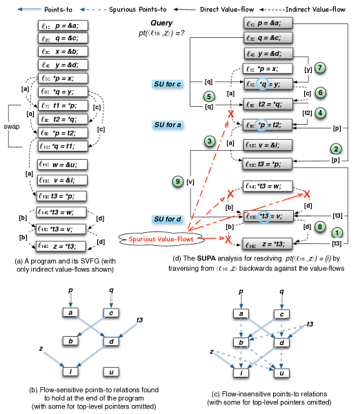
Figure 6: A motivating example for illustrating Supa (SU stands for “Strong Update”).

3 A MOTIVATING EXAMPLE

Our demand-driven pointer analysis, Supa, operates on the SVFG of a program. It computes points-to queries flow- and context-sensitively on-demand by performing strong updates, whenever possible, to refine away imprecise value-flows in the SVFG.

Our example program, shown in Figure 6(a), is simple (even with 16 lines). The program consists of a straight-line sequence of code, with $\ell_{1}$ – $\ell_{10}$ taken directly from Figure 2(b) and the six new statements $\ell_{11}$ – $\ell_{16}$ added to enable us to highlight some key properties of Supa. We assume that $u$ at $\ell_{11}$ is uninitialized but $i$ at $\ell_{12}$ is initialized. The SVFG embedded in Figure 6(a) will be referred to shortly below. We describe how Supa can be used to prove that $z$ at $\ell_{16}$ points only to the initialized object $i$, by computing flow-sensitively on-demand the points-to query $\emph{pt}(\langle\ell_{16},z\rangle)$, i.e., the points-to set of $z$ at the program point after $\ell_{16}$, which is defined in (1) in Section 4.

Figure 6(b) depicts the points-to relations for the six address-taken variables and some top-level ones found at the end of the code sequence by a whole-program flow-sensitive analysis (with strong updates) like SFS [17]. Due to flow-sensitivity, multiple solutions for a pointer are maintained. In this example, these are the true relations observed at the end of program execution. Note that SFS gives rise to Figure 2(c) by analyzing $\ell_{1}$ – $\ell_{6}$, Figure 2(d) by analyzing also $\ell_{7}$ – $\ell_{10}$, and finally, Figure 6(b) by analyzing $\ell_{11}$ – $\ell_{16}$ further. As $z$ points to $i$ but not $u$, no warning is issued for $z$, implying that $z$ is regarded as being properly initialized.

Figure 6(c) shows how the points-to relations in Figure 6(b) are over-approximated flow-insensitively by applying Andersen’s analysis [3]. In this case, a single solution is computed conservatively for the entire program. Due to the lack of strong updates in analyzing the two stores performed by swap, the points-to relations in Figures 2(c) and 2(d) are merged, causing $*a$ and $*c$ to become spurious aliases. When $\ell_{11}$ – $\ell_{16}$ are analyzed, the seven spurious points-to relations (shown in dashed arrows in Figure 6(c)) are introduced. Since $z$ points to $i$ (correctly) and $u$ (spuriously), a false alarm for $z$ will be issued. Failing to consider flow-sensitivity, Andersen’s analysis is not precise for this uninitialization pointer detection client.

Let us now explain how Supa, shown in Figure 1, works. Supa will first perform a pre-analysis to the example program to build the SVFG given in Figure 6(a), as discussed in Section 2. For its top-level variables, their direct value-flows, i.e., def-use chains are explicit and thus omitted to avoid cluttering. For example, $q$ has three def-use chains $\ell_{2}\xrightarrow{q}\ell_{6}$, $\ell_{2}\xrightarrow{q}\ell_{8}$ and $\ell_{2}\xrightarrow{q}\ell_{10}$. For its address-taken variables, there are nine indirect value-flows, i.e., def-use chains depicted in Figure 6(a). Let us see how the two def-use chains for $b$ are created. As $t3$ points to $b$, $\ell_{14}$, $\ell_{15}$ and $\ell_{16}$ will be annotated with $b=\chi(b)$, $b=\chi(b)$ and $\mu(b)$, respectively. By putting $b$ in SSA form, these three functions become $b2=\chi(b1)$, $b3=\chi(b2)$ and $\mu(b3)$. Hence, we have $\ell_{14}\!\xrightarrow{b}\!\ell_{15}$ and $\ell_{15}\!\xrightarrow{b}\!\ell_{16}$, indicating $b$ at $\ell_{16}$ has two potential definitions, with the one at $\ell_{15}$ overwriting the one at $\ell_{14}$. The def-use chains for $d$ and $a$ are built similarly.

Let us consider a single-stage analysis with $\textbf{{Stage[N-1]}}=\textbf{{Stage[0]}}\!=\!FS$ in Figure 1. Figure 6(d) shows how Supa computes $\emph{pt}(\langle\ell_{16},z\rangle)$ on-demand, starting from $\ell_{16}$, by performing a backward reachability analysis on the SVFG, with the visiting order of def-use chains marked as – . Formally, this is done as illustrated in Figure 8. The def-use chains for only the relevant top-level variables are shown. By filtering out the four spurious value-flows (marked by $\mathbin{\leavevmode\hbox to5.34pt{\vbox to5.34pt{\text{[drawing]}}}}$), Supa finds that only $i$ at $\ell_{12}$ is backward reachable from $z$ at $\ell_{16}$. Thus, $\emph{pt}(\langle\ell_{16},z\rangle)=\{i\}$. So no warning for $z$ will be issued.

Supa differs from prior work in the following three major aspects:

• On-Demand Strong Updates

  A whole-program flow-sensitive analysis like SFS [17] can answer $\emph{pt}(\langle\ell_{16},z\rangle)$ precisely but must accomplish this task by analyzing all the 16 statements, resulting in a total of six strong updates performed at the six stores, with some strong updates performed unnecessarily for this query. Unfortunately, existing whole-program FSCS or even just FS algorithms do not scale well for large C programs [1].

  In contrast, Supa computes $\emph{pt}(\langle\ell_{16},z\rangle)$ precisely by performing only three strong updates at $\ell_{6}$, $\ell_{9}$ and $\ell_{15}$. The earlier a strong update is performed by Supa during its reachability analysis, the fewer the number of statements traversed. After – have been performed, Supa finds that $t3$ points to $d$ only. With a strong update performed at $\ell_{15}:*t3=v$ ( ), Supa concludes that $\emph{pt}(\langle\ell_{16},z\rangle)\!=\!\{i\}$.

• Value-Flow Refinement

  Demand-driven pointer analyses [40, 43, 59, 64, 67] are flow-insensitive and thus suffer from the same imprecision as their flow-insensitive whole-program counterparts. In the absence of strong updates, many spurious aliases (such as $*a$ and $*c$) result, causing $z$ to point to both $i$ and $u$. As a result, a false alarm for $z$ is issued, as discussed earlier.

  However, Supa performs strong updates flow-sensitively by filtering out the four spurious pre-computed value-flows marked by $\mathbin{\leavevmode\hbox to5.34pt{\vbox to5.34pt{\text{[drawing]}}}}$. As $t3$ points to $d$ only, $\ell_{15}\!\xrightarrow{b}\!\ell_{16}$ is spurious and not traversed. In addition, a strong update is enabled at $\ell_{15}:*t3=v$, rendering $\ell_{14}\!\xrightarrow{b}\!\ell_{15}$ and $\ell_{14}\!\xrightarrow{d}\!\ell_{15}$ spurious. Finally, $\ell_{5}\!\xrightarrow{a}\!\ell_{9}$ is refined away due to another strong update performed at $\ell_{9}$. Thus, Supa has avoided many spurious aliases (e.g., $*a$ and $*c$) introduced flow-insensitively by pre-analysis, resulting in $\emph{pt}(\langle\ell_{16},z\rangle)\!=\!\{i\}$ precisely. Thus, no warning for $z$ is issued.

• Query-based Precision Control

  To balance efficiency and precision, Supa operates in a hybrid multi-stage analysis framework. When asked to answer the query $\emph{pt}(\langle\ell_{16},z\rangle)$ under a budget, say, a maximum sequence of three steps traversed, Supa will stop its traversal from $\ell_{9}$ to $\ell_{8}$ (at ) in Figure 6(d) and fall back to the pre-computed results by returning $\emph{pt}({\langle\ell_{16},z\rangle})=\{u,i\}$. In this case, a false positive for $z$ will end up being reported.

4 DEMAND-DRIVEN STRONG UPDATES

[ADDR] $\frac{\begin{array}[c]{c}\begin{tabular}[]{lll}$\ell:p=\&o$\end{tabular}\end{array}}{\begin{array}[c]{c}\begin{tabular}[]{ll}$\langle\ell,p\rangle\hookleftarrow\widehat{o}$\end{tabular}\end{array}}$   [COPY] $\frac{\begin{array}[c]{c}\begin{tabular}[]{lll}$\ell:p=q$ \quad$\ell^{\prime}\xrightarrow{q}\ell$\end{tabular}\end{array}}{\begin{array}[c]{c}\begin{tabular}[]{ll}$\langle\ell,p\rangle\hookleftarrow\langle\ell^{\prime},q\rangle$\end{tabular}\end{array}}$

[PHI] $\frac{\begin{array}[c]{c}\begin{tabular}[]{lll}$\ell:p=\phi(q,r)$\quad$\ell^{\prime}\xrightarrow{q}\ell$ \quad$\ell^{\prime\prime}\xrightarrow{r}\ell$\end{tabular}\end{array}}{\begin{array}[c]{c}\begin{tabular}[]{ll}$\langle\ell,p\rangle\hookleftarrow\langle\ell^{\prime},q\rangle$ \quad$\langle\ell,p\rangle\hookleftarrow\langle\ell^{\prime\prime},r\rangle$\end{tabular}\end{array}}$

[FIELD] $\frac{\begin{array}[c]{c}\begin{tabular}[]{lll}$\ell:p=\&q\!\rightarrow\!fld$ \quad$\ell^{\prime}\xrightarrow{q}\ell$ \quad$\langle\ell^{\prime},q\rangle\hookleftarrow\widehat{o}$\end{tabular}\end{array}}{\begin{array}[c]{c}\begin{tabular}[]{ll}$\langle\ell,p\rangle\hookleftarrow\widehat{o_{fld}}$\end{tabular}\end{array}}$

[LOAD] $\frac{\begin{array}[c]{c}\begin{tabular}[]{lll}$\ell:p=*q$ \ \ $\ell^{\prime\prime}\xrightarrow{q}\ell$ \ \ $\langle\ell^{\prime\prime},q\rangle\hookleftarrow\widehat{o}$ \ \ $\ell^{\prime}\xrightarrow{o}\ell$\end{tabular}\end{array}}{\begin{array}[c]{c}\begin{tabular}[]{ll}$\langle\ell,p\rangle\hookleftarrow\langle\ell^{\prime},o\rangle$\end{tabular}\end{array}}$

[STORE] $\frac{\begin{array}[c]{c}\begin{tabular}[]{lll}$\ell:*p=q$ \ \ $\ell^{\prime\prime}\xrightarrow{p}\ell$ \ \ $\langle\ell^{\prime\prime},p\rangle\hookleftarrow\widehat{o}$ \ \ $\ell^{\prime}\xrightarrow{q}\ell$\end{tabular}\end{array}}{\begin{array}[c]{c}\begin{tabular}[]{ll}$\langle\ell,o\rangle\hookleftarrow\langle\ell^{\prime},q\rangle$\end{tabular}\end{array}}$

[SU/WU] $\frac{\begin{array}[c]{c}\begin{tabular}[]{lll}$\ell:*p=\_$ \quad\quad$\ell^{\prime}\xrightarrow{o}\ell$\quad\quad$o\in\mathcal{A}\backslash\ \!\textsl{kill}(\ell,p)$\end{tabular}\end{array}}{\begin{array}[c]{c}\begin{tabular}[]{ll}$\langle\ell,o\rangle\hookleftarrow\langle\ell^{\prime},o\rangle$\end{tabular}\end{array}}$

[CALL] $\frac{\begin{array}[c]{c}\begin{tabular}[]{lll}$\ell:\_=q(\dots,r,\dots)\quad{\color[rgb]{0.00,0.47,0.00}{\color[rgb]{0.00,0.47,0.00}\bm{\mu}}(o_{j})}$ \qquad\quad$\ell^{\prime}:f(\dots,r^{\prime},\dots)\quad{\color[rgb]{0.00,0.47,0.00}o_{i+1}\!=\!{\color[rgb]{0.00,0.47,0.00}\bm{\chi}}(o_{i})}$\\ \qquad\qquad$\ell^{\prime\prime}\xrightarrow{q}\ell$ \quad$\langle\ell^{\prime\prime},q\rangle\hookleftarrow\widehat{o_{f}}$ \quad$\ell\xrightarrow{r}\ell^{\prime}$ \quad$\ell\xrightarrow{o}\ell^{\prime}$\end{tabular}\end{array}}{\begin{array}[c]{c}\begin{tabular}[]{ll}$\langle\ell^{\prime},r^{\prime}\rangle\hookleftarrow\langle\ell,r\rangle$ \quad$\langle\ell^{\prime},o\rangle\hookleftarrow\langle\ell,o\rangle$\\ \end{tabular}\end{array}}$

[RET] $\frac{\begin{array}[c]{c}\begin{tabular}[]{lll}$\ell:p=q(\dots)\quad{\color[rgb]{0.00,0.47,0.00}o_{j+1}\!=\!{\color[rgb]{0.00,0.47,0.00}\bm{\chi}}(o_{j})}$ \qquad\quad$\ell^{\prime}:ret_{f}\ p^{\prime}\quad{\color[rgb]{0.00,0.47,0.00}{\color[rgb]{0.00,0.47,0.00}\bm{\mu}}(o_{i})}$\\ \qquad\qquad$\ell^{\prime\prime}\xrightarrow{q}\ell$ \quad$\langle\ell^{\prime\prime},q\rangle\hookleftarrow\widehat{o_{f}}$ \quad$\ell^{\prime}\xrightarrow{p^{\prime}}\ell$ \quad$\ell^{\prime}\xrightarrow{o}\ell$\end{tabular}\end{array}}{\begin{array}[c]{c}\begin{tabular}[]{ll}$\langle\ell,p\rangle\hookleftarrow\langle p^{\prime},\ell^{\prime}\rangle$ \quad$\langle\ell,o\rangle\hookleftarrow\langle\ell^{\prime},o\rangle$\\ \end{tabular}\end{array}}$

[COMPO] $\frac{\begin{array}[c]{c}\begin{tabular}[]{lll}${lv}\hookleftarrow{lv}^{\prime}$ \hskip 14.22636pt${lv}^{\prime}\hookleftarrow{lv}^{\prime\prime}$\end{tabular}\end{array}}{\begin{array}[c]{c}\begin{tabular}[]{ll}${lv}\hookleftarrow{lv}^{\prime\prime}$\end{tabular}\end{array}}$

$\textsl{kill}(\ell,p)=\begin{cases}\{o^{\prime}\}&\text{if $\emph{pt}(\langle\ell,p\rangle)\!=\!\{o^{\prime}\}\wedge o^{\prime}\in\textsl{singletons}$}\\ \mathcal{A}&\text{else if $\emph{pt}(\langle\ell,p\rangle)\!=\!\varnothing$}\\ \varnothing&\text{otherwise}\end{cases}$

Figure 7: Single-stage flow-sensitive Supa analysis with demand-driven strong updates.

We introduce our demand-driven pointer analysis with strong updates, as illustrated in Figure 1. We first describe our inference rules in a flow-sensitive setting (Section 4.1). We then discuss our context-sensitive extension (Section 4.2). Finally, we present our hybrid multi-stage analysis framework (Section 4.3). All our analyses are field-sensitive, thereby enabling more strong updates to be performed to struct objects.

4.1 Formalism: Flow-Sensitivity

We present a formalization of a single-stage Supa consisting of only a flow-sensitive (FS) analysis. Given a program, Supa will operate on its SVFG representation $G_{{\rm vfg}}$ constructed by applying Andersen’s analysis [3] as a pre-analysis, as discussed in Section 2.4 and illustrated in Section 3.

Let $\mathbb{V}\!=\!\mathcal{L}\times\mathcal{V}$ be the set of labeled variables $lv$, where $\mathcal{L}$ is the set of statement labels and $\mathcal{V}=\mathcal{P}\cup\mathcal{O}$ as defined in Table 1. Supa conducts a backward reachability analysis flow-sensitively on $G_{{\rm vfg}}$ by computing a reachability relation, $\hookleftarrow\ \subseteq\mathbb{V}\times\mathbb{V}$. In our formalism, $\langle\ell,v\rangle\hookleftarrow\langle\ell^{\prime},v^{\prime}\rangle$ signifies a value-flow from a def of $v^{\prime}$ at $\ell^{\prime}$ to a use of $v$ at $\ell$ through one or multiple value-flow paths in $G_{{\rm vfg}}$. For an object $o$ created at an AddrOf statement, i.e., an allocation site at $\ell^{\prime}$, identified as $\langle\ell^{\prime},o\rangle$, we must distinguish it from $\langle\ell,o\rangle$ accessed elsewhere at $\ell$ in our inference rules. Our abbreviation for $\langle\ell^{\prime},o\rangle$ is $\widehat{o}$.

Given a points-to query $\langle\ell,v\rangle$, Supa computes $\emph{pt}(\langle\ell,v\rangle)$, i.e., the points-to set of $\langle\ell,v\rangle$ by finding all reachable target objects $\widehat{o}$, defined as follows:

$$\emph{pt}(\langle\ell,v\rangle)=\{o\mid\langle\ell,v\rangle\hookleftarrow\widehat{o}\}$$ (1)

Despite flow-sensitivity, our formalization in Figure 7 makes no explicit references to program points. As Supa operates on the def-use chains in $G_{{\rm vfg}}$, each variable $\langle\ell,v\rangle$ mentioned in a rule appears at the point just after $\ell$, where $v$ is defined.

Let us examine our rules in detail. By [ADDR], an object $\widehat{o}$ created at an allocation site $\ell$ is backward reachable from $p$ at $\ell$ (or precisely at the point after $\ell$). The pre-computed direct value-flows across the top-level variables in $G_{{\rm vfg}}$ are always precise ([COPY] and [PHI]). In partial SSA form, [PHI] exists only for top-level variables (Section 2.4).

However, the indirect value-flows across the address-taken variables in $G_{{\rm vfg}}$ can be imprecise; they need to be refined on the fly to remove the spurious aliases thus introduced. When handling a load $p=*q$ in [LOAD], we can traverse backwards from $p$ at $\ell$ to the def of $o$ at $\ell^{\prime}$ only if $o$ is actually used by, i.e., aliased with $*q$ at $\ell$, which requires the reachability relation $\langle\ell^{\prime\prime},q\rangle\hookleftarrow\widehat{o}$ to be computed recursively. A store $*p=q$ is handled similarly ([STORE]): $q$ defined at $\ell^{\prime}$ can be reached backwards by $o$ at $\ell$ only if $o$ is aliased with $*p$ at $\ell$.

If $*q$ in a load $\cdots=*q$ is aliased with $*p$ in a store $*p=\cdots$ executed earlier, then $p$ and $q$ must be both backward reachable from $\widehat{o}$. Otherwise, any alias relation established between $*p$ and $*q$ in $G_{{\rm vfg}}$ by pre-analysis must be spurious and will thus be filtered out by value-flow refinement.

[SU/WU] models strong and weak updates at a store $\ell\!:\!p\!=\!\_$. Defining its kill set $\textsl{kill}(\ell,p)$ involves three cases. In Case (1), $p$ points to one singleton object $o^{\prime}$ in singletons, which contains all objects in $\mathcal{A}$ except the local variables in recursion, arrays (treated monolithically) or heap objects [25]. In Section 4.2, we discuss how to apply strong updates to heap objects context-sensitively. A strong update is then possible to $o$. By killing its old contents at $\ell^{\prime}$, no further backward traversal along the def-use chain $\ell^{\prime}\xrightarrow{o}\ell$ is needed. Thus, $\langle\ell,o\rangle\hookleftarrow\langle\ell^{\prime},o\rangle$ is falsified. In Case (2), the points-to set of $p$ is empty. Again, further traversal to $\langle\ell^{\prime},o\rangle$ must be prevented to avoid dereferencing a null pointer as is standard [16, 17, 25]. In Case (3), a weak update is performed to $o$ so that its old contents at $\ell^{\prime}$ are preserved. Thus, $\langle\ell,o\rangle\hookleftarrow\langle\ell^{\prime},o\rangle$ is established, which implies that the backward traversal along $\ell^{\prime}\xrightarrow{o}\ell$ must continue.

[FIELD] handles field-sensitivity. For a field access (e.g., $p=\&q\!\rightarrow\!fld$), pointer $p$ points to the field object $o_{fld}$ of object $o$ pointed to by $q$.

[CALL] and [RET] handle the reachability traversal interprocedurally by computing the call graph for the program on the fly instead of relying on the imprecisely pre-computed call graph built by the pre-analysis as in [17]. In the SVFG, the interprocedural value-flows sinking into a callee function $f$ may come from a spurious indirect callsite $\ell$. To avoid this, both rules ensure that the function pointer $q$ at $\ell$ actually points to $f$ ([CALL] and [RET]). Essentially, given a points-to query $z$ at an indirect callsite $\ell:z=(*fp)()$. Instead of analyzing all the callees found by the pre-analysis, Supa recursively computes the points-to set of $fp$ to discover new callees at the callsite and then continues refining $\emph{pt}(\langle\ell,z\rangle)$ using the new callees.

$\frac{\begin{array}[c]{c}\frac{\begin{array}[c]{c}\ell_{13}:t3=*p\hskip 2.15277pt\ell_{1}\xrightarrow{p}\ell_{13}\hskip 2.15277pt\frac{\begin{array}[c]{c}\ell_{1}:p=\&a\end{array}}{\begin{array}[c]{c}\langle\ell_{1},p\rangle\hookleftarrow\widehat{a}\end{array}}\scalebox{0.78}{{{\small{[{{ADDR}}]}}}}\hskip 2.15277pt\ell_{9}\xrightarrow{a}\ell_{13}\end{array}}{\begin{array}[c]{c}\langle\ell_{13},t3\rangle\hookleftarrow\langle\ell_{9},a\rangle\end{array}}\scalebox{0.78}{{{\small{[{{LOAD}}]}}}}\hskip 3.01389pt\frac{\begin{array}[c]{c}\ell_{9}:*p=t2\hskip 2.15277pt\ell_{1}\xrightarrow{p}\ell_{9}\hskip 2.15277pt\framebox{$\langle\ell_{1},p\rangle\hookleftarrow\widehat{a}$}\hskip 2.15277pt\ell_{8}\xrightarrow{t2}\ell_{9}\end{array}}{\begin{array}[c]{c}\langle\ell_{9},a\rangle\hookleftarrow\langle\ell_{8},t2\rangle\end{array}}\scalebox{0.78}{{{\small{[{{STORE}}]}}}}\end{array}}{\begin{array}[c]{c}\langle\ell_{13},t3\rangle\hookleftarrow\langle\ell_{8},t2\rangle\end{array}}\scalebox{0.78}{{{\small{[{{COMPO}}]}}}}$

(a) Deriving $\emph{pt}(\langle\ell_{13},t3\rangle)$ (corresponding to – in Figure 6(d))

$\frac{\begin{array}[c]{c}\frac{\begin{array}[c]{c}\frac{\begin{array}[c]{c}\langle\ell_{13},\!t3\rangle\hookleftarrow\!\langle\ell_{8},\!t2\rangle\frac{\begin{array}[c]{c}\ell_{8}\!:\!t2\!=\!*q\hskip 2.15277pt\ell_{2}\!\xrightarrow{q}\!\ell_{8}\frac{\begin{array}[c]{c}\ell_{2}\!:\!q\!=\!\&c\end{array}}{\begin{array}[c]{c}\langle\ell_{2},q\rangle\!\hookleftarrow\!\widehat{c}\end{array}}\scalebox{0.78}{{{\small{[{{ADDR}}]}}}}\ell_{6}\!\xrightarrow{c}\!\ell_{8}\end{array}}{\begin{array}[c]{c}\langle\ell_{8},t2\rangle\!\hookleftarrow\!\langle\ell_{6},c\rangle\end{array}}\scalebox{0.78}{{{\small{[{{LOAD}}]}}}}\end{array}}{\begin{array}[c]{c}\langle\ell_{13},t3\rangle\!\hookleftarrow\!\langle\ell_{6},c\rangle\end{array}}\scalebox{0.78}{{{\small{[{{COMPO}}]}}}}\frac{\begin{array}[c]{c}\ell_{6}\!:\!*q\!=\!y\hskip 2.15277pt\ell_{2}\!\xrightarrow{q}\!\ell_{6}\hskip 2.15277pt\framebox{$\langle\ell_{2},q\rangle\!\hookleftarrow\!\widehat{c}$}\hskip 2.15277pt\ell_{4}\!\xrightarrow{y\!}\ell_{6}\end{array}}{\begin{array}[c]{c}\langle\ell_{6},\!c\!\rangle\hookleftarrow\!\langle\ell_{4},\!y\rangle\end{array}}\scalebox{0.78}{{{\small{[{{STORE}}]}}}}\end{array}}{\begin{array}[c]{c}\langle\ell_{13},\!t3\rangle\hookleftarrow\!\langle\ell_{4},\!y\rangle\end{array}}\scalebox{0.78}{{{\small{[{{COMPO}}]}}}}\frac{\begin{array}[c]{c}\ell_{4}\!:\!y\!=\!\&d\end{array}}{\begin{array}[c]{c}\langle\ell_{4},\!y\rangle\hookleftarrow\!\widehat{d}\end{array}}\scalebox{0.78}{{{\small{[{{ADDR}}]}}}}\end{array}}{\begin{array}[c]{c}\langle\ell_{13},\!t3\rangle\hookleftarrow\!\widehat{d}\end{array}}\scalebox{0.78}{{{\small{[{{COMPO}}]}}}}$

(b) Deriving $\emph{pt}(\langle\ell_{13},t3\rangle)$ (corresponding to – in Figure 6(d))

$\frac{\begin{array}[c]{c}\frac{\begin{array}[c]{c}\frac{\begin{array}[c]{c}\ell_{16}:z\!=\!*t3\hskip 2.15277pt\ell_{13}\!\xrightarrow{t3}\!\ell_{16}\hskip 2.15277pt\langle\ell_{13},t3\rangle\!\hookleftarrow\!\widehat{d}\hskip 2.15277pt\ell_{15}\xrightarrow{d}\ell_{16}\end{array}}{\begin{array}[c]{c}\langle\ell_{16},z\rangle\!\hookleftarrow\!\langle\ell_{15},d\rangle\end{array}}\scalebox{0.78}{{{\small{[{{LOAD}}]}}}}\hskip 2.15277pt\frac{\begin{array}[c]{c}\ell_{15}:*t3\!=\!v\hskip 2.15277pt\ell_{13}\!\xrightarrow{t3}\!\ell_{15}\ \hskip 2.15277pt\framebox{\!$\langle\ell_{13},t3\rangle\!\hookleftarrow\!\widehat{d}$\!}\hskip 2.15277pt\ell_{12}\!\xrightarrow{v}\!\ell_{15}\end{array}}{\begin{array}[c]{c}\langle\ell_{15},d\rangle\!\hookleftarrow\!\langle\ell_{12},v\rangle\end{array}}\scalebox{0.78}{{{\small{[{{STORE}}]}}}}\end{array}}{\begin{array}[c]{c}\langle\ell_{16},z\rangle\hookleftarrow\langle\ell_{12},v\rangle\end{array}}\scalebox{0.78}{{{\small{[{{COMPO}}]}}}}\hskip 3.01389pt\frac{\begin{array}[c]{c}\ell_{12}:v\!=\!\&i\end{array}}{\begin{array}[c]{c}\langle\ell_{12},v\rangle\hookleftarrow\widehat{i}\end{array}}\scalebox{0.78}{{{\small{[{{ADDR}}]}}}}\end{array}}{\begin{array}[c]{c}\langle\ell_{16},z\rangle\hookleftarrow\widehat{i}\end{array}}\scalebox{0.78}{{{\small{[{{COMPO}}]}}}}$

(c) Deriving $\emph{pt}(\langle\ell_{16},z\rangle)$ (corresponding to – in Figure 6(d))

Figure 8: Reachability derivations for $\emph{pt}(\langle\ell_{16},z\rangle)$ shown in Figure 6(d) (with reuse of cached points-to results inside each box).

Finally, $\hookleftarrow$ is transitive, stated by [COMPO].

Let us try all our rules, by first revisiting our motivating example where strong updates are performed (Example 4.1) and then examining weak updates (Example 4.2).

Example 4.1.

Figure 8 shows how we apply the rules of Supa to answer $\emph{pt}(\langle\ell_{16},z\rangle)$ illustrated in Figure 6(d). [SU/WU] (implicit in these derivations) is applied to $\ell_{6}$, $\ell_{9}$ and $\ell_{15}$ to cause a strong update at each store. At $\ell_{6}$, $\emph{pt}(\langle\ell_{6},q\rangle)=\{c\}$, the old contents in $c$ are killed. At $\ell_{9}$, $\ell_{5}\!\xrightarrow{a}\!\ell_{9}$ becomes spurious since $\langle\ell_{9},a\rangle\!\hookleftarrow\!\langle\ell_{5},a\rangle$ is falsified. At $\ell_{15}$, $\ell_{14}\!\xrightarrow{b}\!\ell_{15}$ and $\ell_{14}\!\xrightarrow{d}\!\ell_{15}$ are filtered out since $\langle\ell_{15},b\rangle{\hookleftarrow}\langle\ell_{14},b\rangle$ and $\langle\ell_{15},d\rangle\!\hookleftarrow\!\langle\ell_{14},d\rangle$ are falsified. Finally, $\ell_{15}\xrightarrow{b}\ell_{16}$ is ignored since $t3$ points to $d$ only ([LOAD]). $\Box$

Supa improves performance by caching points-to results to reduce redundant traversal, with reuse happening in the marked boxes in Figure 8. For example, in Figure 8(c), $\emph{pt}(\langle\ell_{13},t3\rangle)=\{\widehat{d}\}$ computed in [LOAD] is reused in [STORE].

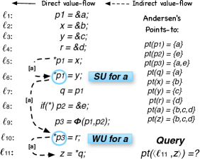
Figure 9: Resolving $\emph{pt}({\langle\ell_{11},z\rangle})=\{c,d\}$ with a weak update.

Example 4.2.

Let us consider a weak update example in Figure 9 by computing $\emph{pt}(\langle\ell_{11},z\rangle)$ on-demand. At the confluence point $\ell_{9}$, $p3$ receives the points-to information from both $p1$ and $p2$ in its two branches: $\langle\ell_{9},p_{3}\rangle\hookleftarrow\widehat{a}$ and $\langle\ell_{9},p_{3}\rangle\hookleftarrow\widehat{e}$. Thus, a weak update is performed to the two locations ${a}$ and ${e}$ at $\ell_{10}$. Let us focus on $\widehat{a}$ only. By applying [STORE], $\langle\ell_{10},a\rangle\hookleftarrow\langle\ell_{4},r\rangle\hookleftarrow\widehat{d}$. By applying [SU/WU], $\langle\ell_{10},a\rangle\hookleftarrow\langle\ell_{6},a\rangle\hookleftarrow\langle\ell_{3},y\rangle\hookleftarrow\widehat{c}$. Thus, $\emph{pt}(\langle\ell_{11},a\rangle)=\{c,d\}$, which excludes $b$ due to a strong update performed at $\ell_{6}$. As $\emph{pt}(\langle\ell_{7},q\rangle)=\{a\}$, we obtain $\emph{pt}(\langle\ell_{11},z\rangle)=\{c,d\}$. $\Box$

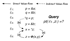
Figure 10: Resolving $\emph{pt}(\langle\ell_{5},z\rangle)\!=\!\{a,b\}$ in a value-flow cycle.

Unlike [25], which falls back to the flow-insensitive points-to information for all weakly updated objects, Supa handles them as precisely as (whole-program) flow-sensitive analysis subject to a sufficient budget. In Figure 9, due to a weak update performed to $a$ at $\ell_{10}$, pt$(\langle\ell_{10},a\rangle)=\{c,d\}$ is obtained, forcing their approach to adopt $\emph{pt}(\langle\ell_{10},a\rangle)=\{b,c,d\}$ thereafter, causing pt$(\langle\ell_{11},z\rangle)=\{b,c,d\}$. By maintaining flow-sensitivity with a strong update applied to $\ell_{6}$ to kill $b$, Supa obtains pt$(\langle\ell_{11},z\rangle)=\{c,d\}$ precisely.

4.1.1 Handling Value-Flow Cycles

To compute soundly and precisely the points-to information in a value-flow cycle in the SVFG, Supa retraverses it whenever new points-to information is found until a fix point is reached.

Example 4.3.

Figure 10 shows a value-flow cycle formed by $\ell_{5}\xrightarrow{x}\ell_{6}$ and $\ell_{6}\xrightarrow{z}\ell_{5}$. To compute pt$(\langle\ell_{6},z\rangle)$, we must compute pt$(\langle\ell_{5},x\rangle)$, which requires the aliases of $*z$ at the load $\ell_{5}:x=*z$ to be found by using pt$(\langle\ell_{6},z\rangle)$. Supa computes pt$(\langle\ell_{6},z\rangle)$ by analyzing this value-flow cycle in two iterations. In the first iteration, a pointed-to target $\widehat{b}$ is found since $\langle\ell_{6},z\rangle\hookleftarrow\langle\ell_{4},y\rangle\hookleftarrow\widehat{b}$. Due to $\langle\ell_{2},q\rangle\hookleftarrow\widehat{b}$, $*z$ and $*q$ are found to be aliases. In the second iteration, another target $\widehat{a}$ is found since $\langle\ell_{6},z\rangle\hookleftarrow\langle\ell_{5},x\rangle\hookleftarrow\langle\ell_{3},b\rangle\hookleftarrow\langle\ell_{1},p\rangle\hookleftarrow\widehat{a}$. Thus, pt$(\langle\ell_{6},z\rangle)=\{a,b\}$ is obtained. $\Box$

4.1.2 Field-Sensitivity

Field-insensitive pointer analysis does not distinguish different fields of a struct object, and consequently, gives up opportunities for performing strong updates to a struct object, as a struct object may actually represent its distinct fields. In contrast, Supa is truly field-sensitive, by avoiding the two limitations altogether.

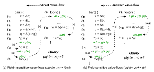
Figure 11: Resolving $\emph{pt}(\langle\ell_{11},r\rangle)\!=\!\{c\}$ with field-sensitivity.

Example 4.4.

Figure 11 illustrates the effects of field-sensitivity on computing the points-to information for $r$ at $\ell_{11}$. Without field-sensitivity, as illustrated in Figure 11(a), the two statements at $\ell_{4}$ and $\ell_{5}$ are analyzed as if they were $\ell_{4}:p=\&x$ and $\ell_{5}:q=\&x$. As a result, no strong update is possible at $\ell_{6}$ and $\ell_{7}$, since $x$, which represents possibly multiple fields, is not a singleton. Thus, $\emph{pt}(\langle\ell_{11},r\rangle)=\{b,c\}$.

Supa is field-sensitive. To answer the points-to query for $r$ at $\ell_{11}$, we compute first $\langle\ell_{11},r\rangle\hookleftarrow\langle\ell_{10},w\rangle$ and then $\langle\ell_{10},v\rangle\hookleftarrow\langle\ell_{9},v\rangle\hookleftarrow\langle\ell_{8},x\rangle\hookleftarrow\langle\ell_{1},x\rangle\hookleftarrow{\widehat{a}}$. By applying [FIELD] at $\ell_{10}$ and [LOAD] at $\ell_{11}$, we obtain $\langle\ell_{11},r\rangle\hookleftarrow\langle\ell_{11},a.g\rangle$. By traversing the three indirect def-use chains for $a.g$, $\ell_{7}\xrightarrow{b.g}\ell_{8}$, $\ell_{8}\xrightarrow{a.g}\ell_{9}$ and $\ell_{9}\xrightarrow{a.g}\ell_{11}$, backwards from $\ell_{11}$, we obtain $\emph{pt}(\langle\ell_{11},r\rangle)\hookleftarrow\langle\ell_{9},a.g\rangle\hookleftarrow\langle\ell_{8},a.g\rangle\hookleftarrow\langle\ell_{7},a.g\rangle\hookleftarrow{\langle\ell_{3},z\rangle}\hookleftarrow{\widehat{c}}$. $\Box$

4.1.3 Properties

Theorem 4.5 (Soundness).

Supa is sound in analyzing a program as long as its pre-analysis (for computing the SVFG of the program) is sound.

Proof 4.6.

When building the SVFG for a program, the def-use chains for its top-level variables are identified explicitly in its partial SSA form. If the pre-analysis (for computing the sparse value-flow graph of the program) is sound, then the def-use chains built for all the address-taken variables are over-approximate. According to its inference rules in Figure 4, Supa performs essentially a flow-sensitive analysis on-demand, by restricting the propagation of points-to information along the precomputed def-use chains, and falls back to the sound points-to information computed by the pre-analysis when running out of its given budgets. Thus, Supa is sound if the pre-analysis is sound.

Theorem 4.7 (Precision).

Given a points-to query $\langle\ell,v\rangle$, $\emph{pt}(\langle\ell,v\rangle)$ computed by Supa is the same as that computed by (whole-program) FS if Supa can successfully resolve the points-to query within a given budget.

Proof 4.8.

Let $\emph{pt}_{\textsc{Supa}}(\langle\ell,v\rangle)$ and $\emph{pt}_{\textsc{FS}}(\langle\ell,v\rangle)$ be the points-to sets computed by Supa and FS, respectively. By Theorem 1, $\emph{pt}_{\textsc{Supa}}(\langle\ell,v\rangle)\supseteq\emph{pt}_{\textsc{FS}}(\langle\ell,v\rangle)$, since Supa is a demand-driven version of FS and thus cannot be more precise. To show that $\emph{pt}_{\textsc{Supa}}(\langle\ell,v\rangle)\subseteq\emph{pt}_{\textsc{FS}}(\langle\ell,v\rangle)$, we note that Supa operates on the SVFG of the program to improve its efficiency, by also filtering out value-flows imprecisely pre-computed by the pre-analysis. For the top-level variables, their direct value-flows are precise. So Supa proceeds exactly the same as FS ([ADDR], [COPY], [PHI], [FIELD], [CALL], [RET] and [COMPO]). For the address-taken variables, Supa establishes the same indirect value-flows flow-sensitively as FS does but in a demand-driven manner, by refining away imprecisely pre-computed value-flows ([LOAD], [STORE], [SU/WU], [CALL], [RET] and [COMPO]). If Supa can complete its query within the given budget, then $\emph{pt}_{\textsc{Supa}}(\langle\ell,v\rangle)\subseteq\emph{pt}_{\textsc{FS}}(\langle\ell,v\rangle)$. Thus, $\emph{pt}_{\textsc{Supa}}(\langle\ell,v\rangle)=\emph{pt}_{\textsc{FS}}(\langle\ell,v\rangle)$.

[C-ADDR] $\frac{\begin{array}[c]{c}\begin{tabular}[]{lll}$c,\ell:p=\&o$\end{tabular}\end{array}}{\begin{array}[c]{c}\begin{tabular}[]{ll}$\langle c,\ell,p\rangle\hookleftarrow(c,\widehat{o})$\end{tabular}\end{array}}$ [C-COPY] $\frac{\begin{array}[c]{c}\begin{tabular}[]{lll}$c,\ell:p=q$ \quad$\ell^{\prime}\xrightarrow{q}\ell$\end{tabular}\end{array}}{\begin{array}[c]{c}\begin{tabular}[]{ll}$\langle c,\ell,p\rangle\hookleftarrow\langle c,\ell^{\prime},q\rangle$\end{tabular}\end{array}}$

[C-PHI] $\frac{\begin{array}[c]{c}\begin{tabular}[]{lll}$c,\ell:p=\phi(q,r)$ \quad$\ell^{\prime}\xrightarrow{q}\ell$ \quad$\ell^{\prime\prime}\xrightarrow{r}\ell$\end{tabular}\end{array}}{\begin{array}[c]{c}\begin{tabular}[]{ll}$\langle c,\ell,p\rangle\hookleftarrow\langle c,\ell^{\prime},q\rangle$ \quad$\langle c,\ell,p\rangle\hookleftarrow\langle c,\ell^{\prime\prime},r\rangle$\end{tabular}\end{array}}$

[C-FIELD] $\frac{\begin{array}[c]{c}\begin{tabular}[]{lll}$c,\ell:p=\&q\!\rightarrow\!fld$ \quad$\ell^{\prime}\xrightarrow{q}\ell$ \quad$\langle c,\ell^{\prime},q\rangle\hookleftarrow(c^{\prime},\widehat{o})$\end{tabular}\end{array}}{\begin{array}[c]{c}\begin{tabular}[]{ll}$\langle c,\ell,p\rangle\hookleftarrow(c^{\prime},\widehat{o.fld})$\end{tabular}\end{array}}$

[C-LOAD] $\frac{\begin{array}[c]{c}\begin{tabular}[]{lll}$c,\ell:p=*q$ \ \ $\ell^{\prime\prime}\xrightarrow{q}\ell$ \ \ $\langle c,\ell^{\prime\prime},q\rangle\hookleftarrow(c^{\prime},\widehat{o})$ \ \ $\ell^{\prime}\xrightarrow{o}\ell$\end{tabular}\end{array}}{\begin{array}[c]{c}\begin{tabular}[]{ll}$\langle c,\ell,p\rangle\hookleftarrow\langle c^{\prime},\ell^{\prime},o\rangle$\end{tabular}\end{array}}$

[C-STORE] $\frac{\begin{array}[c]{c}\begin{tabular}[]{lll}$c,\ell:*p=q$ \ \ $\ell^{\prime\prime}\xrightarrow{p}\ell$ \ \ $\langle c,\ell^{\prime\prime},p\rangle\hookleftarrow(c^{\prime},\widehat{o})$ \ \ $\ell^{\prime}\xrightarrow{q}\ell$\end{tabular}\end{array}}{\begin{array}[c]{c}\begin{tabular}[]{ll}$\langle c^{\prime},\ell,o\rangle\hookleftarrow\langle c,\ell^{\prime},q\rangle$\\ \end{tabular}\end{array}}$

[C-SU/WU] $\frac{\begin{array}[c]{c}\begin{tabular}[]{lll}$c,\ell:*p=\_$ \quad$\ell^{\prime}\xrightarrow{o}\ell$ \quad\quad$(c^{\prime},o)\in\mathcal{A}\backslash\ \!\textsl{kill}(c,\ell,p)$\end{tabular}\end{array}}{\begin{array}[c]{c}\begin{tabular}[]{ll}$\langle c^{\prime},\ell,o\rangle\hookleftarrow\langle c^{\prime},\ell^{\prime},o\rangle$\end{tabular}\end{array}}$

[C-COMPO] $\frac{\begin{array}[c]{c}\begin{tabular}[]{lll}${lv}\hookleftarrow{lv}^{\prime}$ \hskip 2.84526pt${lv}^{\prime}\hookleftarrow{lv}^{\prime\prime}$\end{tabular}\end{array}}{\begin{array}[c]{c}\begin{tabular}[]{ll}${lv}\hookleftarrow{lv}^{\prime\prime}$\end{tabular}\end{array}}$

[C-CALL] $\frac{\begin{array}[c]{c}\begin{tabular}[]{lll}$c,\ell:\_=q(\dots,r,\dots)\quad{\color[rgb]{0.00,0.47,0.00}{\color[rgb]{0.00,0.47,0.00}\bm{\mu}}(o_{j})}$ \qquad\quad$\ell^{\prime\prime}\xrightarrow{q}\ell$ \ $\langle c,\ell^{\prime\prime},q\rangle\hookleftarrow(\_,\widehat{o_{f}})$ \ $\ell\xrightarrow{r}\ell^{\prime}$ \ $\ell\xrightarrow{o}\ell^{\prime}$\\ $c^{\prime},\ell^{\prime}:f(\dots,r^{\prime},\dots)\quad{\color[rgb]{0.00,0.47,0.00}o_{i+1}\!=\!{\color[rgb]{0.00,0.47,0.00}\bm{\chi}}(o_{i})}$ \qquad\quad$c=c^{\prime}\ominus\ell$\end{tabular}\end{array}}{\begin{array}[c]{c}\begin{tabular}[]{ll}$\langle c^{\prime},\ell^{\prime},r^{\prime}\rangle\hookleftarrow\langle c,\ell,r\rangle$ \quad$\langle c^{\prime},\ell^{\prime},o\rangle\hookleftarrow\langle c,\ell,o\rangle$\\ \end{tabular}\end{array}}$

[C-RET] $\frac{\begin{array}[c]{c}\begin{tabular}[]{lll}$c,\ell:p=q(\dots)\ {\color[rgb]{0.00,0.47,0.00}o_{j+1}\!=\!{\color[rgb]{0.00,0.47,0.00}\bm{\chi}}(o_{j})}$ \qquad\quad$\ell^{\prime\prime}\xrightarrow{q}\ell$ \ $\langle c,\ell^{\prime\prime},q\rangle\hookleftarrow(\_,\widehat{o_{f}})$ \ $\ell^{\prime}\xrightarrow{p^{\prime}}\ell$ \ $\ell^{\prime}\xrightarrow{o}\ell$\\ $c^{\prime},\ell^{\prime}:ret_{f}\ p^{\prime}\quad{\color[rgb]{0.00,0.47,0.00}{\color[rgb]{0.00,0.47,0.00}\bm{\mu}}(o_{i})}$ \qquad\qquad\qquad\quad$c^{\prime}=c\oplus\ell$\end{tabular}\end{array}}{\begin{array}[c]{c}\begin{tabular}[]{ll}$\langle c,\ell,p\rangle\hookleftarrow\langle c^{\prime},p^{\prime},\ell^{\prime}\rangle$ \quad$\langle c,\ell,o\rangle\hookleftarrow\langle c^{\prime},\ell^{\prime},o\rangle$\\ \end{tabular}\end{array}}$

$\textsl{kill}(c,\ell,p)=\begin{cases}\{(c^{\prime},o^{\prime})\}&\text{if $\emph{pt}(\langle c,\ell,p\rangle)\!=\!\{(c^{\prime},o^{\prime})\}\wedge(c^{\prime},o^{\prime})\in\textsl{cxtSingletons}$}\\ \mathcal{A}&\text{else if $\emph{pt}(\langle c,\ell,p\rangle)\!=\!\varnothing$}\\ \varnothing&\text{otherwise}\end{cases}$

Figure 12: Single-stage flow- and context-sensitive Supa analysis with demand-driven strong updates.

4.2 Formalism: Flow- and Context-Sensitivity

We extend our flow-sensitive formalization by considering also context-sensitivity to enable more strong updates (especially now for heap objects). We solve a balanced-parentheses problem by matching calls and returns to filter out unrealizable inter-procedural paths [29, 39, 40, 43, 59]. A context stack $c$ is encoded as a sequence of callsites, [$\kappa_{1}\dots\kappa_{m}$], where $\kappa_{i}$ is a call instruction $\ell$. $c\oplus\kappa$ denotes an operation for pushing a callsite $\kappa$ into $c$. $c\ominus\kappa$ pops $\kappa$ from $c$ if $c$ contains $\kappa$ as its top value or is empty since a realizable path may start and end in different functions.

With context-sensitivity, a statement is parameterized additionally by a context $c$, e.g., $c,\ell\!:\!p\!=\!\&o$, to represent its instance when its containing function is analyzed under $c$. A labeled variable $lv$ has the form $\langle c,\ell,v\rangle$, representing variable $v$ accessed at statement $\ell$ under context $c$. An object $\widehat{o}$ that is created at an AddrOf statement under context $c$ is also context-sensitive, identified as $(c,\widehat{o})$.

Given a points-to query $\langle c,\ell,v\rangle$, Supa computes its points-to set both flow- and context-sensitively by applying the rules given in Figure 12:

$$\emph{pt}(\langle c,\ell,v\rangle)=\{(c^{\prime},o)\mid\langle c,\ell,v\rangle\hookleftarrow(c^{\prime},\widehat{o})\}$$ (2)

where the reachability relation $\hookleftarrow$ is now also context-sensitive.

Passing parameters to and returning results from a callee invoked at a callsite are handled by [C-CALL] and [C-RET]. [C-CALL] deals with the direct and indirect value-flows backwards from the entry instruction of a callee function to each of its callsites based on the call graph computed on the fly similarly as [CALL] in Figure 7, except that [C-CALL] is context-sensitive. Likewise, [C-RET] deals with the direct and indirect value-flows backwards from a callsite to the return instruction of every callee function.

With context-sensitivity, Supa will filter out more spurious value-flows generated by Andersen’s analysis, thereby producing more precise points-to information to enable more strong updates ([C-SU/WU]). At a store $c,\ell:*p=\_$, its kill set is context-sensitive. A strong update is applied if $p$ points to a context-sensitive singleton $(c^{\prime},o^{\prime})\in\textsl{cxtSingletons}$, where $o^{\prime}$ is a (non-heap) singleton defined in Section 4.1 or a heap object with $c^{\prime}$ being a concrete context, i.e., one not involved in recursion or loops.

Example 4.9.

Let us use an example given in Figure 13 to illustrate the effects of context-sensitive strong updates on computing the points-to information for $z$ at $\ell_{5}$. This example is adapted from a real application, milc-v6, given in Figure 17(c). Without context-sensitivity, Supa will only perform a weak update at $\ell_{8}:*x=y$, since $x$ points to both $a$ and $b$ passed into foo() from the two callsites at $\ell_{3}$ and $\ell_{4}$. As a result, $z$ at $\ell_{5}$ is found to point to not only what $y$ points to, i.e., $c$ but also what $b$ points to previously (not shown to avoid cluttering). With context-sensitivity, Supa finds that $\langle[\ ],\ell_{5},z\rangle\hookleftarrow\langle[\ ],\ell_{5},b\rangle\hookleftarrow\langle[\ ],\ell_{4},b\rangle\hookleftarrow\langle[\ell_{4}],\ell_{9},b\rangle\hookleftarrow\langle[\ell_{4}],\ell_{8},b\rangle\hookleftarrow\langle[\ell_{4}],\ell_{7},y\rangle\hookleftarrow([\ell_{4}],\widehat{c})$. Since $\langle[\ell_{4}],\ell_{8},x\rangle$ points to a context-sensitive singleton $(\ell_{4},b)$ at $\ell_{8}$, a strong update is performed to $b$ at $\ell_{8}$, causing the old contents in $b$ to be killed. $\Box$

Given a program, the SCCs (strongly connected components) in its call graph are constructed on the fly. Supa handles the SCCs in the program context-sensitively but the function calls inside a SCC context-insensitively as in [43].

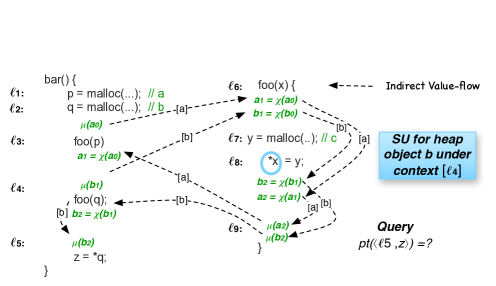
Figure 13: Resolving $\emph{pt}([\ ],\ell_{5},z)=\{[\ell_{4}],c\}$) with context-sensitive strong updates.

4.3 SUPA: Hybrid Multi-Stage Analysis

To facilitate efficiency and precision tradeoffs in answering on-demand queries, Supa, as illustrated in Figure 1, organizes its analyses in multiple stages sorted in increasing efficiency but decreasing precision. Let there be $M$ queries issued successively. Let the $N$ stages of Supa, $\textbf{{Stage[0]}},\cdots,\textbf{{Stage[N-1]}}$, be configured with budgets $\eta_{0},\cdots,\eta_{N-1}$, respectively. In our current implementation, each budget is specified as the maximum number of def-use chains traversed in the SVFG of the program.

Supa answers a query on-demand by applying its $N$ analyses successively, starting from Stage[0]. If the query is not answered after budget $\eta_{i}$ has been exhausted at stage $i$, Supa re-issues the query at stage $i+1$, and eventually falls back to the results that are pre-computed by pre-analysis.

Supa caches fully computed points-to information in a query and reuses it in subsequent queries, as illustrated in Figure 8. Let $\mathcal{Q}$ be the set of queried variables issued from a program. Let $\mathcal{I}\supseteq\mathcal{Q}$ be the set of variables reached from $\mathcal{Q}$ during the analysis. Let $(\ell,v)\in\mathcal{Q}$ be a queried variable. We write $\emph{pt}_{\eta_{i}}^{i}(\langle\Delta_{i},\ell,v\rangle)$ to represent the points-to set of a variable $\langle\ell,v\rangle$ computed at stage $i$ under budget $\eta_{i}$, where $\Delta_{i}$ is a contextual qualifier at stage $i$ (e.g., $c$ in FSCS). By convention, $\emph{pt}_{\eta_{N}}^{N}(\langle\Delta_{N},\ell,v\rangle)$ denotes the points-to set obtained by pre-analysis, at Stage[N] (conceptually).

When resolving $\emph{pt}_{\eta_{i}}^{i}(\langle\Delta_{i},\ell,v\rangle)$ at stage $i$, suppose Supa has reached a variable $\langle\ell^{\prime},v^{\prime}\rangle\in\mathcal{I}$ and needs to compute $\emph{pt}_{*}^{i}(\langle\Delta_{i},\ell^{\prime},v^{\prime}\rangle)$, where $*(\leqslant\eta_{i}$) represents an unknown budget remaining, with $(\ell^{\prime},v^{\prime})$ being $(\ell,v)$ possibly (in a cycle).

Presently, Supa exploits two types of reuse to improve efficiency with no loss of precision in a hybrid manner:

Backward Reuse: $(\ell^{\prime},v^{\prime})\in\mathcal{I}$

If $\emph{pt}_{*}^{j}(\langle\Delta_{j},\ell^{\prime},v^{\prime}\rangle)$, where $j\leqslant i$, was previously cached, then $\emph{pt}_{*}^{i}(\langle\Delta_{i},\ell^{\prime},v^{\prime}\rangle)=\emph{pt}_{*}^{j}(\langle\Delta_{j},\ell^{\prime},v^{\prime}\rangle)$, provided that $\emph{pt}_{*}^{j}(\langle\Delta_{j},\ell^{\prime},v^{\prime}\rangle)$ is a sound representation of $\emph{pt}_{*}^{i}(\langle\Delta_{i},\ell^{\prime},v^{\prime}\rangle)$. For example, if $\textbf{{Stage[i]}}=FS$ and $\textbf{{Stage[j]}}=FSCS$, then $\emph{pt}_{*}^{FSCS}(\langle c^{\prime},\ell^{\prime},v^{\prime}\rangle)$ can be reused for $\emph{pt}_{*}^{FS}(\langle\ell^{\prime},v^{\prime}\rangle)$ if $c^{\prime}$ is true, representing a context-free points-to set.

Forward Reuse: $(\ell^{\prime},v^{\prime})\in\mathcal{Q}$

If $\emph{pt}_{\eta_{j}}^{j}(\langle\Delta_{j},\ell^{\prime},v^{\prime}\rangle)$, where $j>i$, was previously computed and cached but $\emph{pt}_{\eta_{k}}^{k}(\langle\Delta_{k},\ell^{\prime},v^{\prime}\rangle)$ was not, where $0\leqslant k<j$, then Supa will also fail for $\emph{pt}_{*}^{k}(\langle\Delta_{k},\ell^{\prime},v^{\prime}\rangle)$, where $i\leqslant k<j$, since $*\leqslant\eta_{k}$. Therefore, Supa will exploit the second type of reuse by setting $\emph{pt}_{*}^{i}(\langle\Delta_{i},\ell^{\prime},v^{\prime}\rangle)=\emph{pt}_{\eta_{j}}^{j}(\langle\Delta_{j},\ell^{\prime},v^{\prime}\rangle)$.

Of course, many other schemes are possible with or without precision loss.

5 EVALUATION

We evaluate Supa by choosing detection of uninitialized pointers as a major client. The objective is to show that Supa is effective in answering client queries, in environments with small time and memory budgets such as IDEs, by facilitating efficiency and precision tradeoffs in a hybrid multi-stage analysis framework. We provide evidence to demonstrate a good correlation between the number of strong updates performed on-demand and the degree of precision achieved during the analysis.

5.1 Implementation

We have implemented Supa in LLVM (3.5.0). The source files of a program are compiled under “-O0” (to facilitate detection of undefined values [66]) into bit-code by clang and then merged using the LLVM Gold Plugin at link time to produce a whole program bc file. The compiler option mem2reg is applied to promote memory into registers. Otherwise, SUPA will perform more strong updates on memory locations that would otherwise be promoted to registers, favoring SUPA undesirably.

All the analyses evaluated are field-sensitive.

Positive weight cycles that arise from processing fields of struct objects are collapsed [36]. Arrays are considered monolithic so that the elements in an array are not distinguished. Distinct allocation sites (i.e., AddrOf statements) are modeled by distinct abstract objects.

We build the SVFG for a program based on our open-source software, SVF [50]. The def-use chains are pre-computed by Andersen’s algorithm flow and context-insensitively. In order to compute soundly and precisely the points-to information in a value-flow cycle, Supa retraverses the cycle whenever new points-to information is discovered until a fix point is reached.

To compare Supa with whole-program analysis, we have implemented a sparse flow-sensitive (SFS) analysis described in [17] also in LLVM, as SFS is a recent solution yielding exactly the flow-sensitive precision with good scalability. However, there are some differences. In [17], SFS was implemented in LLVM (2.5.0), by using imprecisely pre-computed call graphs and representing points-to sets with binary decision diagrams (BDDs). In this paper, just like Supa, SFS is implemented in LLVM (3.5.0), by building a program’s call graph on the fly (Section 4.1) and representing points-to sets with sparse bit vectors.

We have not implemented a whole-program FSCS pointer analysis in LLVM. There is no open-source implementation either in LLVM. According to [1], existing FSCS algorithms for C “do not scale even for an order of magnitude smaller size programs than those analyzed” by Andersen’s algorithm. As shown here, SFS can already spend hours on analyzing some programs under 500 KLOC.

5.2 Methodology

We choose uninitialized pointer detection as a major client, named Uninit, which requires strong update analysis to be effective. As a common type of bugs in C programs, uninitialized pointers are dangerous, as dereferencing them can cause system crashes and security vulnerabilities. For Uninit, flow-sensitivity is crucial. Otherwise, strong updates are impossible, making Uninit checks futile.

We will show that Supa can answer Uninit’s on-demand queries efficiently while achieving nearly the same precision as SFS. For C, global and static variables are default initialized, but local variables are not. In order to mimic the default uninitialization at a stack or heap allocation site $\ell\!:\!p\!=\!\&a$ for an uninitialized pointer $a$, we add a special store $*p\!=\!u$ immediately after $\ell$, where $u$ points to an unknown abstract object (UAO), $u_{a}$. Given a load $x\!=\!*y$, we can issue a points-to query for $x$ to detect its potential uninitialization. If $x$ points to a $u_{a}$ (for some $a$), then $x$ may be uninitialized. By performing strong updates more often, a flow-sensitive analysis can find more UAO’s that do not reach any pointer and thus prove more pointers to be initialized. Note that SFS can yield false positives since, for example, path correlations are not modeled.

We do not introduce UAO’s for the local variables involved in recursion and array objects since they cannot be strongly updated. We also ignore all the default-initialized stack or heap objects (e.g., those created by calloc()).

Table 3: Program characteristics.

Program	KLOC	Statements	Pointers	Allocation Sites	Queries
spell-1.1	0.8	1011	1274	42	17
bc-1.06	14.4	17018	15212	654	689
milc-v6	15	11713	29584	865	3
less-451	27.1	6766	22835	1135	100
sed-4.2	38.6	25835	34226	395	1191
hmmer-2.3	36	27924	74689	1472	2043
make-4.1	40.4	14926	36707	1563	1133
gzip-1.6	64.4	22028	25646	1180	551
a2ps-4.14	64.6	49172	116129	3625	5065
bison-3.0.4	113.3	36815	90049	1976	4408
grep-2.21	118.4	10199	33931	1108	562
tar-1.28	132	30504	85727	3350	909
wget-1.16	140.0	51556	63199	726	1142
bash-4.3	155.9	59442	191413	6359	5103
gnugo-3.4	197.2	369741	286986	27511	1970
sendmail-8.15	259.9	86653	256074	7549	2715
vim-7.4	413.1	147550	466493	8960	6753
emacs-24.4	431.9	189097	754746	12037	4438
Total	2263.0	1157950	2584920	80507	38792

We generate meaningful points-to queries, one query for the top-level variable $x$ at each load $x\!=\!*y$. However, we ignore this query if $x$ is found not to point to any UAO by pre-analysis. This happens only when $x$ points to either default-initialized objects or unmodeled local variables in recursion cycles or arrays. The number of queries issued in each program is listed in the last column in Table 3.

5.3 Experimental Setup

We use a machine with a 3.7GHz Intel Xeon 8-core CPU and 64 GB memory. As shown in Table 3, we have selected a total of 18 open-source programs from a variety of domains: spell-1.1 (a spelling checker), bc-1.06 (a numeric processing language), milc-v6 (quantum chromodynamics), less-451 (a terminal pager), sed-4.2 (a stream editor), milc-v6 (quantum chromodynamics), hmmer-2.3 (sequence similarity searching), make-4.1 (a build automation tool), a2ps-4.14 (a postScript filter), bison-3.04 (a parser), grep-2.2.1 (string searching), tar-1.28 (tar archiving), wget-1.16 (a file downloading tool), bash-4.3 (a unix shell and command language), gnugo-3.4 (a Go game), sendmail-8.15.1 (an email server and client), vim74 (a text editor), and emacs-24.4 (a text editor).

For each program, Table 3 lists its number of lines of code, statements which are LLVM instructions relevant to our pointer analysis, pointers, allocation sites (or AddrOf statements), and queries issued (as discussed in Section 5.2).

5.4 Results and Analysis

We evaluate Supa with two configurations, Supa-FS and Supa-FSCS. Supa-FS is a one-stage FS analysis by considering flow-sensitivity only. Supa-FSCS is a two-stage analysis consisting of FSCS and FS applied in that order.

5.4.1 Evaluating Supa-FS

When assessing Supa-FS, we consider two different criteria: efficiency (its analysis time and memory usage per query) and precision (its competitiveness against SFS). For each query, its analysis budget, denoted $B$, represents the maximum number of def-use chains that can be traversed. We consider a wide range of budgets with $B$ falling into $[10,200000]$.

Supa-FS is highly effectively. With $B=10000$, Supa-FS is nearly as precise as SFS, by consuming about 0.18 seconds and 65KB of memory per query, on average.

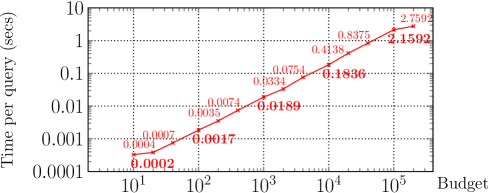
(a) Analysis Time

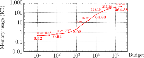
(b) Memory Usage

Figure 14: Average analysis time and memory usage per query consumed by Supa-FS under different analysis budgets (with both axes being logarithmic).

Table 4: Pre-processing times taken by pre-analysis shared by Supa and SFS and analysis times of SFS (in seconds).

Program	Pre-Analysis Times			Analysis Time of SFS
	Shared by Supa and SFS
	Andersen’s Analysis	SVFG	Total
spell	0.01	0.01	0.01	0.01
bc	0.35	0.21	0.56	0.98
milc	0.42	0.1	0.52	0.16
less	0.42	0.37	0.79	1.94
sed	1.38	0.34	1.73	5.46
hmmer	1.57	0.46	2.03	1.07
make	1.74	1.17	2.91	13.94
gzip	0.27	0.10	0.37	0.20
a2ps	7.34	1.31	8.65	60.61
bison	8.18	3.66	11.84	44.16
grep	1.44	0.17	1.61	2.39
tar	2.73	1.71	4.44	12.27
wget	1.86	0.90	2.76	3.47
bash	53.48	44.07	97.55	2590.69
gnugo	5.68	2.75	8.44	9.86
sendmail	24.05	23.43	47.48	348.63
vim	445.88	85.69	531.57	13823
emacs	135.93	146.94	282.87	8047.55

Efficiency

Figure 14(a) shows the average analysis time per query for all the programs under a given budget, with about 0.18 seconds when $B\!=\!10000$ and about 2.76 seconds when $B\!=\!200000$. Both axes are logarithmic. The longest-running queries can take an order of magnitude as long as the average cases. However, most queries (around 80% across the programs) take much less than the average cases. Take emacs for example. SFS takes over two hours (8047.55 seconds) to finish. In contrast, Supa-FS spends less than ten minutes (502.10 seconds) when $B\!=\!2000$, with an average per-query time (memory usage) of 0.18 seconds (0.12KB), and produces the same answers for all the queries as SFS (shown in Figure 15 and explained below).

For Supa, its pre-analysis is lightweight, as shown in Table 4, with vim taking the longest at 531.57 seconds. The same pre-analysis is also shared by SFS in order to enable its own sparse whole-program analysis. The additional time taken by SFS for analyzing each program entirely is given in the last column.

Figure 14(b) shows the average memory usage per query under different budgets. Following the common practice, we measure the real-time memory usage by reading the virtual memory information (VmSize) from the linux kernel file (/proc/self/status). The memory monitor starts after the pre-analysis to measure the memory usage for answering queries only. The average amount of memory consumed per query is small, with about 65KB when $B=10000$ and about 436KB when $B\!=\!200000$. Even under the largest budget $B=200000$ evaluated, Supa-FS never uses more than 3MB for any single query processed.

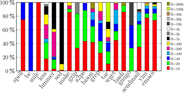
Figure 15: Percentage of queried variables proved to be initialized by Supa-FS over SFS under different budgets.

Precision

Given a query $\emph{pt}({\langle\ell,p\rangle}$), $p$ is initialized if no UAO is pointed by $p$ and potentially uninitialized otherwise. We measure the precision of Supa-FS in terms of the percentage of queried variables proved to be initialized by comparing with SFS, which yields the best precision achievable as a whole-program flow-sensitive analysis.

Figure 15 reports our results. As $B$ increases, the precision of Supa-FS generally improves. With $B\!=\!10000$, Supa-FS can answer correctly 97.4% of all the queries from the 18 programs. These results indicate that our analysis is highly accurate, even under tight budgets. For the 18 programs except a2ps, bison and bash, Supa-FS produces the same answers for all the queries when $B=100000$ as SFS. When $B=200000$ for these three programs, Supa becomes as precise as SFS, by taking an average of 0.02 seconds (88.5KB) for a2ps, 0.25 seconds (194.7KB) for bison, and 3.18 seconds (1139.3KB) for bash, per query.

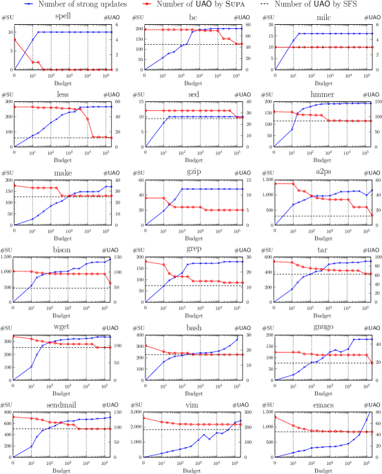
Figure 16: Correlating the number of strong updates with the number of UAO’s under Supa-FS with different analysis budgets.

Understanding On-Demand Strong Updates

Let us examine the benefits achieved by Supa-FS in answering client queries by applying on-demand strong updates. For each program, Figure 16 shows a good correlation between the number of strong updates performed (#SU on the left y-axis) in a blue curve and the number of UAO’s reaching some uninitialized pointers (#UAO on the right y-axis) in a red curve under varying budgets (on the logarithmic x-axis). The number of such UAO’s reported by SFS is shown as the lower bound for Supa-FS in a dashed line.

In most programs, Supa-FS performs increasingly more strong updates to block increasingly more UAO’s to reach the queried variables as the analysis budget $B$ increases, because Supa-FS falls back increasingly less frequently from FS to the pre-computed points-to information. When $B$ increases, Supa-FS can filter out more spurious value-flows in the SVFG to obtain more precise points-to information, thereby enabling more strong updates to kill the UAO’s.

When $B=200000$, Supa-FS gives the same answers as SFS in all the 18 programs except bison and vim, which causes Supa-FS to report 16 and 35 more, respectively.

For some programs such as spell, bc, milc, hmmer and grep, most of their strong updates happen under small budgets (e.g., $B=1000$). In hmmer, for example, 192 strong updates are performed when $B=10000$. Of the 5126 queries issued, Supa-FS runs out-of-budget for only three queries, which are all fully resolved when $B=200000$, but with no further strong updates being observed.

For programs like bison, bash, gnugo and emacs, quite a few strong updates take place when $B>1000$. There are two main reasons. First, these programs have many indirect call edges (with 8709 in bison, 1286 in bash, 23150 in gnugo and 4708 in emacs), making their on-the-fly call graph construction costly (Section 4.1.2). Second, there are many value-flow cycles (with over 50% def-use chains occurring in cycles in bison), making their constraint resolution costly (to reach a fixed point). Therefore, relatively large budgets are needed to enable more strong updates to be performed.

Interestingly, in programs such as a2ps, gnugo and vim, fewer strong updates are observed when larger budgets are used. In vim, the number of strong updates performed is 1492 when $B=2000$ but drops to 1204 when $B=4000$. This is due to the forward reuse described in Section 4.3. When answering a query $\emph{pt}(\langle\ell,v\rangle)$ under two budgets $B_{1}$ and $B_{2}$, where $B_{1}<B_{2}$, Supa-FS has reached $\langle\ell^{\prime},v^{\prime}\rangle$ and needs to compute $\emph{pt}(\langle\ell^{\prime},v^{\prime}\rangle)$ in each case. Supa-FS may fall back to the flow-insensitive points-to set of $v^{\prime}$ under $B_{1}$ but not $B_{2}$, resulting in more strong updates performed under $B_{1}$ in the part of the program that is not explored under $B_{2}$.

5.4.2 Evaluating Supa-FSCS

For C programs, flow-sensitivity is regarded as being important for achieving useful high precision. However, context-sensitivity can be important for some C programs, in terms of both obtaining more precise points-to information and enabling more strong updates. Unfortunately, whole-program analysis does not scale well to large programs when both are considered (Section 5.1).

Table 5: Average analysis times consumed and UAO’s reported by Supa-FSCS (with a budget of 10000 in each stage) and Supa-FS (with a budget of 10000 in total).

Program	Supa-FS		Supa-FSCS
	Time (ms)	$\#\textsf{UAO}$	Time (ms)	$\#\textsf{UAO}$
spell	0.01	0	0.01	0
bc	18.35	69	287.23	69
milc	0.02	3	14.52	0
less	15.15	37	92.41	37
sed	355.60	32	4725.42	32
hmmer	11.41	86	135.05	71
make	124.40	26	229.44	26
gzip	0.64	5	4.28	5
a2ps	126.01	34	448.26	32
bison	465.54	94	529.20	86
grep	124.46	14	197.66	14
tar	26.31	70	83.10	68
wget	24.51	104	84.90	104
bash	188.69	17	327.16	17
gnugo	72.73	28	80.08	27
sendmail	200.32	94	250.19	85
vim	168.67	218	473.25	218
emacs	159.22	45	222.65	45

In this section, we demonstrate that Supa can exploit both flow- and context-sensitivity effectively on-demand in a hybrid multi-stage analysis framework, providing improved precision needed by some programs. Table 5 compares Supa-FSCS (with a budget of 20000 divided evenly in its FSCS and FS stages) with Supa-FS (with a budget of 10000 in its single FS stage). The maximal depth of a context stack allowed is 3. By allocating the budgets this way, we can investigate some additional precision benefits achieved by considering both flow- and context-sensitivity.

In general, Supa-FSCS has longer query response times than Supa-FS due to the larger budgets used in our setting and the times taken in handling context-sensitivity. In milc, hmmer, a2ps, bison, tar , gnugo and sendmail, Supa-FSCS reports fewer UAO’s than Supa-FS, for two reasons. First, Supa-FSCS can perform strong updates context-sensitively for stack and global objects, resulting in 0 UAO’s reported by Supa-FSCS for milc. Second, Supa-FSCS can perform strong updates to context-sensitive singleton heap objects defined in Section 4.2, by eliminating 8 UAO’s in bison, 1 in tar and 1 in sendmail, which have been reported by Supa-FS.

6 Case Studies

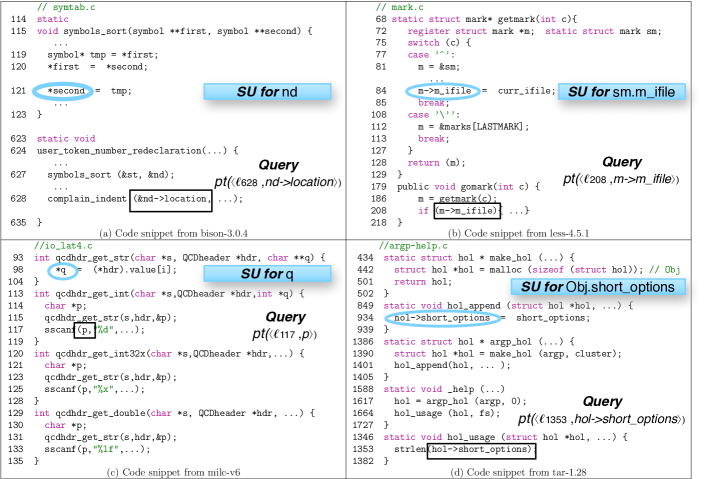
Figure 17: Selected code snippets.

We examine some real code to see how client queries are answered precisely with on-demand strong updates under four different scenarios.

Figure 17(a)

There is a swap from bison. In line 121, second points to a singleton stack object nd passed from line 627. So a strong update is applied. When querying nd->location in line 628, Supa knows that nd points to what st pointed to before.

Figure 17(b)

In the code fragment from less, m->m_ifile is initialized in two different branches, one recognized due to a strong update performed at the store in line 84 and one due to the default initialization in line 112. According to Supa, m->m_ifile in line 208 is initialized.

Figure 17(c)

In the code fragment from milc, q in line 98 can point to several stack variables that are all named $p$ in lines 115, 123 and 131. With context-sensitivity, Supa finds that q points to one singleton under each context. Thus, a strong update is performed so that each stack variable becomes properly initialized when queried at each call to sscanf().

Figure 17(d)

In the code fragment from tar, hol in line 1390 points to a heap object $o$ allocated in line 442. With $o$ treated as a context-sensitive singleton (requiring a context stack of at least depth 1), a strong update can be performed in line 934 to initialize its field short_options properly.

7 Parallelizing Supa

To demonstrate that Supa is amenable to parallelization as a demand-driven analysis, we have parallelized Supa-FS by using Intel Threading Building Blocks (TBB). A concurrent_queue is used to store all the queries issued from a program. We use a task_group to allocate tasks for computing the queries from concurrent_queue in parallel. The cached points-to information is shared with a concurrent_hash_map.

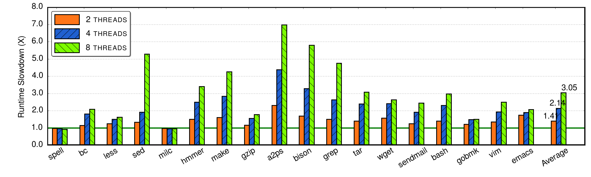
Figure 18: Speedups of Supa-FS when parallelized over its sequential version with two, four and eight threads ($B=10000)$.

Figure 18 shows the speedups achieved by parallelization over the sequential setting with $B=10000$. With eight threads, the average speedup for the 18 programs is 3.05x and the maximum speedup observed is 6.9x at a2ps. The time for each setting excludes the pre-analysis time. Some programs enjoy better speedups than others. There are three main reasons. First, some programs, such as spell, less and milc, have relatively few queries issued. Therefore, the performance benefits achieved from query parallelization can be small. Second, different queries take different times to answer, resulting in different degrees of workload imbalance in different programs. Third, different programs suffer from different synchronization overheads in accessing the cached points-to information in concurrent_hash_map.

8 RELATED WORK

Demand-driven and whole-program approaches represent two important solutions to long-standing pointer analysis problems. While a whole-program pointer analysis aims to resolve all the pointers in the program, a demand-driven pointer analysis is designed to resolve only a (typically small) subset of the set of these pointers in a client-specific manner. This work is not concerned with developing an ultra-fast whole-program pointer analysis. Rather, our objective is to design a staged demand-driven strong update analysis framework that facilitates efficiency and precision tradeoffs flow- and context-sensitively according to the needs of a client (e.g., user-specified budgets). Below we limit our discussion to the work that is most relevant to Supa.

8.1 Flow-Sensitive Pointer Analysis

Strong updates require pointers to be analyzed flow-sensitively with respect to program execution order. Whole-program flow-sensitive pointer analysis has been studied extensively in the literature. Choi et al., 1993 and Emami and Hendren, 1994 gave some formulations in an iterative data-flow framework [21]. Wilson and Lam, 1995 considered both flow- and context-sensitivity by representing procedure summaries with partial transfer functions, but restricted strong updates to top-level variables only. To eliminate unnecessary propagation of points-to information during the iterative data-flow analysis [63, 16, 17, 35], some form of sparsity has been exploited. The sparse value-flows, i.e., def-use chains in a program are captured by sparse evaluation graphs (SEG) [8, 38] as in [19] and various SSA representations such as HSSA [9], partial SSA [24] and SSI [2, 56]. The def-use chains for top-level pointers, once put in SSA, can be explicitly and precisely identified, giving rise to a so-called semi-sparse flow-sensitive analysis [16]. Later, the idea of staged analysis [14] has been leveraged to make pointer analysis full-sparse for both top-level and address-taken variables by using fast Andersen’s analysis as precise analysis [47, 62, 17]. This paper is the first to exploit sparsity to improve the performance of a flow- and context-sensitive demand-driven analysis with strong updates being performed for C programs.

Recently, Balatsouras and Smaragdakis [5] propose a fine-grained field-sensitive modeling technique for performing Andersen’s analysis by inferring lazily the types of heap objects in order to filter out redundant field derivations. This technique can be exploited to obtain a more precise pre-analysis to improve the precision and/or efficiency of sparse flow-sensitive analysis.

8.2 Demand-Driven Pointer Analysis

Demand-driven pointer analyses for C [18, 67, 64] and Java [29, 40, 59, 43, 46] are flow-insensitive, formulated in terms of CFL (Context-Free-Language) reachability [39]. Heintze and Tardieu, 2001 introduced the first on-demand Andersen-style pointer analysis for C. Later, Zheng and Rugina, 2008 performed alias analysis for C in terms of CFL-reachability flow- and context-insensitively with indirect function calls handled conservatively. Sridharan et al. gave two CFL-reachability-based formulations for Java, initially without considering context-sensitivity [44] and later with context-sensitivity [43]. Shang et al., 2012 and Yan et al.,  2011 investigated how to summarize points-to information discovered during the CFL-reachability analysis to improve performance for Java programs. Lu et al., 2013 introduced an incremental pointer analysis with a CFL-reachability formulation for Java. Su et al., 2014 demonstrated that the CFL-reachability formulation is highly amenable to parallelization on multi-core CPUs. Recently, Feng et al., 2015 focused on answering demand queries for Java programs in a context-sensitive analysis framework (without performing strong updates). Unlike these flow-insensitive analyses, which are not effective for many clients like Uninit, Supa can perform strong updates on-demand flow and context-sensitively.

Boomerang [42] represents a recent flow- and context-sensitive demand-driven pointer analysis for Java. However, its access-path-based analysis performs only strong updates partially at a store $a.f=\dots$, by updating $a.f$ strongly but the aliases of $a.f.*$ weakly, where $a$ and $b$ are different top-level variables. Let us explain this by using the following straight-line Java code and its corresponding C code.

Java Code $\ell_{1}$: q = new A()    // o1 $\ell_{2}$: p = q $\ell_{3}$: p.f = new A()  // o2 $\ell_{4}$: q.f = new A()  // o3 $\ell_{5}$: x = p.f

C Code $\ell_{1}$: q = malloc()    // o1 $\ell_{2}$: p = q $\ell_{3}$: *p = malloc()  // o2 $\ell_{4}$: *q = malloc()  // o3 $\ell_{5}$: x = *p

Let us consider Boomerang first. At $\ell_{3}$, a strong update is performed to $p.f$ to make it point to $o2$ only. At $\ell_{4}$, a strong update is performed to $q.f$ to make it point to $o3$ but a weak update is performed to all its aliases so that $p.f$ now points to not only $o2$ as before but also $o3$, As a result, $x$ points-to both $o2$ and $o3$ at $\ell_{5}$. Let us consider now Supa. With both flow- and context-sensitivity enforced, a strong update is performed to $o1$ pointed $p$ and $q$ at both $\ell_{3}$ and $\ell_{4}$, respectively. Thus, $x$ points to $o3$ only at $\ell_{5}$.

8.3 Hybrid Pointer Analysis

The basic idea is to find a right balance between efficiency and precision. For C programs, the one-level approach [11] achieves a precision between Steensgaard’s and Andersen’s analyses by applying a unification process to address-taken variables only. In the case of Java programs, context-sensitivity can be made more effective by considering both call-site-sensitivity and object-sensitivity together than either alone [22]. In [15], how to adjust the analysis precision according to a client’s needs is discussed. Zhang et al., 2014b  focus on finding effective abstractions for whole-program analyses written in Datalog via abstraction refinement. Lhoták and Chung [25] trades precision for efficiency by performing strong updates only on flow-sensitive singleton objects but falls back to the flow-insensitive points-to information otherwise. In this paper, we propose to carry out our on-demand strong update analysis in a hybrid multi-stage analysis framework. Unlike [25], Supa can achieve the same precision as whole-program flow-sensitive analysis, subject to a given budget.

8.4 Parallel Pointer Analysis

Méndez-Lojo et al., 2010 introduced a parallel implementation of Andersen’s analysis for C based on graph rewriting. Their parallel analysis is flow- and context-insensitive, achieving a speedup of up to 3X on an 8-core CPU. Su et al., 2016 introduces an improvement of this parallel implementation on GPUs. The whole-program sparse flow-sensitive pointer analysis [16] has also been parallelized on multi-core CPUs [33] and GPUs [34]. The speedups are up to 2.6X on a 8-core CPU. This paper presents the first parallel implementation of demand-driven pointer analysis with strong updates for C programs, achieving an average speedup of 3.05X on a 8-core CPU.

9 Conclusion

We have introduced, Supa, a demand-driven pointer analysis that enables computing precise points-to information for C programs flow- and context-sensitively with strong updates by refining away imprecisely pre-computed value-flows, subject to some analysis budgets. Supa handles large C programs effectively by allowing pointer analyses with different efficiency and precision tradeoffs to be applied in a hybrid multi-stage analysis framework. Supa is particularly suitable for environments with small time and memory budgets such as IDEs. We have evaluated Supa by choosing uninitialized pointer detection as a major client on 18 C programs. Supa can achieve nearly the same precision as whole-program flow-sensitive analysis under small budgets.

One interesting future work is to investigate how to allocate budgets in Supa to its stages to improve the precision achieved in answering some time-consuming queries for a particular client. Another direction is to add more stages to its analysis, by considering, for example, path correlations.

References

- Acharya and Robinson, [2011] Acharya, M. and Robinson, B. (2011). Practical change impact analysis based on static program slicing for industrial software systems. In ICSE ’11, pages 746–755.
- Ananian, [1999] Ananian, C. S. (1999). The static single information form. PhD thesis, Master’s Thesis, MIT.
- Andersen, [1994] Andersen, L. (1994). Program analysis and specialization for the C programming language. PhD thesis, DIKU, University of Copenhagen.
- Arzt et al., [2014] Arzt, S., Rasthofer, S., Fritz, C., Bodden, E., Bartel, A., Klein, J., Le Traon, Y., Octeau, D., and McDaniel, P. (2014). Flowdroid: Precise context, flow, field, object-sensitive and lifecycle-aware taint analysis for android apps. In PLDI ’14, pages 259–269.
- Balatsouras and Smaragdakis, [2016] Balatsouras, G. and Smaragdakis, Y. (2016). Structure-sensitive points-to analysis for c and c++. In SAS ’16.
- Blackshear et al., [2013] Blackshear, S., Chang, B.-Y. E., and Sridharan, M. (2013). Thresher: Precise refutations for heap reachability. In PLDI ’13, pages 275–286.
- Choi et al., [1993] Choi, J.-D., Burke, M., and Carini, P. (1993). Efficient flow-sensitive interprocedural computation of pointer-induced aliases and side effects. In POPL ’93, pages 232–245.
- Choi et al., [1991] Choi, J.-D., Cytron, R., and Ferrante, J. (1991). Automatic construction of sparse data flow evaluation graphs. In POPL ’91, pages 55–66.
- Chow et al., [1996] Chow, F., Chan, S., Liu, S., Lo, R., and Streich, M. (1996). Effective representation of aliases and indirect memory operations in SSA form. In CC ’96, pages 253–267.
- Cytron et al., [1991] Cytron, R., Ferrante, J., Rosen, B., Wegman, M., and Zadeck, F. (1991). Efficiently computing static single assignment form and the control dependence graph. TOPLAS’91, 13(4):490.
- Das, [2000] Das, M. (2000). Unification-based pointer analysis with directional assignments. In PLDI ’00, pages 35–46.
- Emami and Hendren, [1994] Emami, M. Ghiya, R. and Hendren, J. (1994). Context-sensitive interprocedural points-to analysis in presence of function pointers. In PLDI ’94, pages 242–256.
- Feng et al., [2015] Feng, Y., Wang, X., Dillig, I., and Lin, C. (2015). EXPLORER: query- and demand-driven exploration of interprocedural control flow properties. In OOPSLA ’15, pages 520–534.
- Fink et al., [2008] Fink, S. J., Yahav, E., Dor, N., Ramalingam, G., and Geay, E. (2008). Effective typestate verification in the presence of aliasing. ACM TOSEM, 17(2):9.
- Guyer and Lin, [2003] Guyer, S. Z. and Lin, C. (2003). Client-driven pointer analysis. In SAS ’03, pages 1073–1073.
- Hardekopf and Lin, [2009] Hardekopf, B. and Lin, C. (2009). Semi-sparse flow-sensitive pointer analysis. In POPL ’09, pages 226–238.
- Hardekopf and Lin, [2011] Hardekopf, B. and Lin, C. (2011). Flow-Sensitive Pointer Analysis for Millions of Lines of Code. In CGO ’11, pages 289–298.
- Heintze and Tardieu, [2001] Heintze, N. and Tardieu, O. (2001). Demand-driven pointer analysis. In PLDI ’01, pages 24–34.
- Hind and Pioli, [1998] Hind, M. and Pioli, A. (1998). Assessing the effects of flow-sensitivity on pointer alias analyses. In SAS ’98, pages 57–81.
- ISO90, [1990] ISO90 (1990). ISO/IEC. international standard ISO/IEC 9899, programming languages - C.
- Kam and Ullman, [1977] Kam, J. B. and Ullman, J. D. (1977). Monotone data flow analysis frameworks. Acta Informatica, 7(3):305–317.
- Kastrinis and Smaragdakis, [2013] Kastrinis, G. and Smaragdakis, Y. (2013). Hybrid context-sensitivity for points-to analysis. In PLDI ’13, pages 423–434.
- Landi, [1992] Landi, W. (1992). Undecidability of static analysis. ACM Letters on Programming Languages and Systems (LOPLAS), 1(4):323–337.
- Lattner and Adve, [2004] Lattner, C. and Adve, V. (2004). LLVM: A compilation framework for lifelong program analysis & transformation. In CGO ’04, pages 75–86.
- Lhoták and Chung, [2011] Lhoták, O. and Chung, K.-C. A. (2011). Points-to analysis with efficient strong updates. In POPL ’11, pages 3–16.
- Lhoták and Hendren, [2003] Lhoták, O. and Hendren, L. (2003). Scaling Java points-to analysis using Spark. CC ’03, pages 153 – 169.
- Li et al., [2011] Li, L., Cifuentes, C., and Keynes, N. (2011). Boosting the performance of flow-sensitive points-to analysis using value flow. In FSE ’11, pages 343–353.
- Li et al., [2014] Li, Y., Tan, T., Sui, Y., and Xue, J. (2014). Self-inferencing reflection resolution for Java. In ECOOP ’14, pages 27–53.
- Lu et al., [2013] Lu, Y., Shang, L., Xie, X., and Xue, J. (2013). An incremental points-to analysis with CFL-reachability. In CC’13.
- Méndez-Lojo et al., [2010] Méndez-Lojo, M., Mathew, A., and Pingali, K. (2010). Parallel inclusion-based points-to analysis. In OOPSLA ’10, pages 428–443.
- Milanova et al., [2002] Milanova, A., Rountev, A., and Ryder, B. G. (2002). Parameterized object sensitivity for points-to and side-effect analyses for Java. ISSTA ’02.
- Milanova et al., [2005] Milanova, A., Rountev, A., and Ryder, B. G. (2005). Parameterized object sensitivity for points-to analysis for Java. ACM Trans. Softw. Eng. Methodol., 14(1):1–41.
- Nagaraj and Govindarajan, [2013] Nagaraj, V. and Govindarajan, R. (2013). Parallel flow-sensitive pointer analysis by graph-rewriting. In PACT ’13, pages 19–28.
- Nasre, [2013] Nasre, R. (2013). Time- and space-efficient flow-sensitive points-to analysis. TACO ’13, 10(4):39:1–39:27.
- Oh et al., [2012] Oh, H., Heo, K., Lee, W., Lee, W., and Yi, K. (2012). Design and implementation of sparse global analyses for C-like languages. In PLDI ’12, pages 229–238.
- Pearce et al., [2007] Pearce, D., Kelly, P., and Hankin, C. (2007). Efficient field-sensitive pointer analysis of C. ACM TOPLAS, 30(1):4–es.
- Ramalingam, [1994] Ramalingam, G. (1994). The undecidability of aliasing. ACM TOPLAS, 16(5):1467–1471.
- Ramalingam, [2002] Ramalingam, G. (2002). On sparse evaluation representations. Theoretical Computer Science, 277(1):119–147.
- Reps et al., [1995] Reps, T., Horwitz, S., and Sagiv, M. (1995). Precise interprocedural dataflow analysis via graph reachability. In POPL ’95, pages 49–61.
- Shang et al., [2012] Shang, L., Xie, X., and Xue, J. (2012). On-demand dynamic summary-based points-to analysis. In CGO ’12, pages 264–274.
- Smaragdakis et al., [2011] Smaragdakis, Y., Bravenboer, M., and Lhoták, O. (2011). Pick your contexts well: understanding object-sensitivity. In POPL’11, pages 17–30.
- Späth et al., [2016] Späth, J., Do, L. N. Q., Ali, K., and Bodden, E. (2016). Boomerang: Demand-driven flow-and context-sensitive pointer analysis for java. ECOOP.
- Sridharan and Bodík, [2006] Sridharan, M. and Bodík, R. (2006). Refinement-based context-sensitive points-to analysis for Java. PLDI ’06, pages 387–400.
- Sridharan et al., [2005] Sridharan, M., Gopan, D., Shan, L., and Bodík, R. (2005). Demand-driven points-to analysis for Java. In OOPSLA ’05, pages 59–76.
- Su et al., [2014] Su, Y., Ye, D., and Xue, J. (2014). Parallel pointer analysis with cfl-reachability. In ICPP ’14, pages 451–460.
- Su et al., [2016] Su, Y., Ye, D., Xue, J., and Liao, X. (2016). An efficient GPU implementation of inclusion-based pointer analysis. IEEE Trans. Parallel Distrib. Syst., 27(2):353–366.
- [47] Sui, Y., Di, P., and Xue, J. (2016a). Sparse flow-sensitive pointer analysis for multithreaded programs. In CGO ’16, pages 160–170. ACM.
- [48] Sui, Y., Fan, X., Zhou, H., and Xue, J. (2016b). Loop-oriented array-and field-sensitive pointer analysis for automatic simd vectorization. In LCTES ’16, pages 41–51. ACM.
- Sui et al., [2013] Sui, Y., Li, Y., and Xue, J. (2013). Query-directed adaptive heap cloning for optimizing compilers. In CGO ’13, pages 1–11.
- Sui and Xue, [2016] Sui, Y. and Xue, J. (2016). SVF: Interprocedural static value-flow analysis in LLVM. In CC ’16, pages 265–266.
- Sui et al., [2012] Sui, Y., Ye, D., and Xue, J. (2012). Static memory leak detection using full-sparse value-flow analysis. In ISSTA ’12, pages 254–264.
- [52] Sui, Y., Ye, D., and Xue, J. (2014a). Detecting memory leaks statically with full-sparse value-flow analysis. TSE ’14, 40(2):107–122.
- [53] Sui, Y., Ye, S., Xue, J., and Zhang, J. (2014b). Making context-sensitive inclusion-based pointer analysis practical for compilers using parameterised summarisation. SPE ’14, 44(12):1485–1510.
- Sun et al., [2011] Sun, Q., Zhao, J., and Chen, Y. (2011). Probabilistic points-to analysis for Java. In CC ’11, pages 62–81.
- SUPA, [2016] SUPA (2016). SUPA. http://www.cse.unsw.edu.au/~corg/supa.
- Tavares et al., [2014] Tavares, A., Boissinot, B., Pereira, F., and Rastello, F. (2014). Parameterized construction of program representations for sparse dataflow analyses. In CC ’14, pages 18–39. Springer.
- Wilson and Lam, [1995] Wilson, R. and Lam, M. (1995). Efficient context-sensitive pointer analysis for C programs. PLDI ’95, pages 1–12.
- Xiao and Zhang, [2011] Xiao, X. and Zhang, C. (2011). Geometric encoding: forging the high performance context sensitive points-to analysis for Java. In ISSTA ’11, pages 188–198.
- Yan et al., [2011] Yan, D., Xu, G., and Rountev, A. (2011). Demand-driven context-sensitive alias analysis for Java. In ISSTA ’11, pages 155–165.
- Yan et al., [2016] Yan, H., Sui, Y., Chen, S., and Xue, J. (2016). Automated memory leak fixing on value-flow slices for c programs. In Proceedings of the 31st Annual ACM Symposium on Applied Computing, SAC ’16, pages 1386–1393, New York, NY, USA. ACM.
- [61] Ye, D., Sui, Y., and Xue, J. (2014a). Accelerating dynamic detection of uses of undefined variables with static value-flow analysis. In CGO ’14.
- [62] Ye, S., Sui, Y., and Xue, J. (2014b). Region-based selective flow-sensitive pointer analysis. In SAS ’14, pages 319–336.
- Yu et al., [2010] Yu, H., Xue, J., Huo, W., Feng, X., and Zhang, Z. (2010). Level by level: making flow-and context-sensitive pointer analysis scalable for millions of lines of code. In CGO ’10, pages 218–229.
- [64] Zhang, Q., Xiao, X., Zhang, C., Yuan, H., and Su, Z. (2014a). Efficient subcubic alias analysis for C. In PLDI ’14, pages 829–845.
- [65] Zhang, X., Mangal, R., Grigore, R., Naik, M., and Yang, H. (2014b). On abstraction refinement for program analyses in Datalog. In PLDI ’14, pages 239–248.
- Zhao et al., [2012] Zhao, J., Nagarakatte, S., Martin, M. M., and Zdancewic, S. (2012). Formalizing the LLVM intermediate representation for verified program transformations. In POPL ’12, pages 427–440.
- Zheng and Rugina, [2008] Zheng, X. and Rugina, R. (2008). Demand-driven alias analysis for C. In POPL ’08, pages 197–208.