A 3D MHD simulation of SN 1006: a polarized emission study for the turbulent case

Abstract

Three dimensional magnetohydrodynamical simulations were carried out in order to perform a new polarization study of the radio emission of the supernova remnant SN 1006. These simulations consider that the remnant expands into a turbulent interstellar medium (including both magnetic field and density perturbations). Based on the referenced-polar angle technique, a statistical study was done on observational and numerical magnetic field position-angle distributions. Our results show that a turbulent medium with an adiabatic index of 1.3 can reproduce the polarization properties of the SN 1006 remnant. This statistical study reveals itself as a useful tool for obtaining the orientation of the ambient magnetic field, previous to be swept up by the main supernova remnant shock.

1 Introduction

SN 1006 is a young supernova remnant (SNR) that has gained interest due to the large observational data available in a wide wavelength range, therefore serving as an ideal laboratory when trying to understand the observed morphology in each frequency. This remnant is classified as part of the bilateral SNR group, whose main characteristic is the presence of two bright and opposite arcs in radio-frequencies.

The morphology and emission of this type of SNRs is largely determined by the environment in which they evolve, sometimes having an irregular or clumpy background and/or with the presence of density and magnetic fields gradients.

The interstellar medium is known to be turbulent, as inferred from observational data (Lee & Jokipii, 1976) and local information on the interplanetary medium (Jokipii et al., 1969). Such turbulent medium, with a Kolmogorov-like power spectrum that spans over a large range of spatial scales (Guo et al., 2012), gives rise to Rayleigh-Taylor (RT) instabilities during the fast expansion of the SNR, which in turn affects the radio emission and is imprinted in the measured Stokes parameters.

Jun & Jones (1999) performed 2D MHD simulations of the evolution of a young Type Ia SNR interacting with an interstellar cloud. They found that the interaction produced RT instabilities causing amplification of the magnetic field, and subsequently changing the synchrotron brightness. This work emphasized the importance of including a turbulent medium when trying to match observations. In this direction, Balsara et al. (2001) performed more realistic 3D simulations of a SNR evolving in a turbulent background. They found that the variability of the emission during the early phase of SNR evolution gives information about the turbulent environment. At the same time, that the interaction with such a turbulent environment generates an enhanced turbulent post-shock region which has observational consequences, as it affects the acceleration of relativistic particles.

Guo et al. (2012) employed 2D MHD simulations to study the magnetic field amplification mechanisms during the propagation of the SNR blast wave. They found that, for high resolution simulations, magnetic field growth at small scales occurs efficiently in two distinct regions: one related to the shock amplification, and the other, to the RT-instabilities at the contact discontinuity between the shocked ejecta and the shocked interstellar medium.

Fang & Zhang (2012) carried out a study similar to that of Guo et al. (2012) but considering different adiabatic indexes to account for both the diffusive shock acceleration and the escape of the accelerated particles from the shock. They found that a smaller effective adiabatic index produces a larger magnetic field enhancement. They extended their study considering a scenario where the expanding ejecta interacts with a large, dense clump and found, in addition to an increase in the complexity of the magnetic field, the development of a non-thermal emitting filament. In a subsequent study, Fang et al. (2014) performed 3D MHD simulations considering a turbulent medium with a Kolmogorov-like power spectrum with parameters resembling the SNR RX J0852.0-4622. Their X-ray and $\gamma$-ray synthetic maps showed the expected rippled morphology with a broken circular shape along the shell, nicely reproducing the observations.

In general, the diffusive shock acceleration is driven by magnetic fields strong enough to generate non-thermal emission. Therefore, any structure or dynamic interaction that results in the amplification of the magnetic field has important consequences on the observed brightness.

According to the non-thermal radio-emission morphology, SN 1006 has been classified as a bilateral or barrel-shaped SNR (Kesteven & Caswell, 1987), showing two main bright arcs towards the NE and SW. The non-thermal X-ray emission is also predominant in the NE and SW rims (Cassam-Chenaï et al., 2008).

SN 1006 is located at a high Galactic latitude and is therefore thought to be evolving in a fairly homogenous interstellar medium. In Schneiter et al. (2010) and Schneiter et al. (2015) we made use of this assumption and presented studies of the system in 2D and 3D, respectively. In the latter work we further introduced synthetic maps of the Stokes $Q$ and $U$ parameters wich allowed a better and more direct comparison with the observations (Reynoso et al., 2013).

Recently, West et al. (2016b, a) (see also, West et al., 2016a, b) studied radio emission for a sample of Galactic axisymmetric SNRs, including SN 1006. They concluded that the quasi-perpendicular acceleration mechanism can sucessfully fit the observed morphology of the remnants in their sample, although SN 1006 seems to be the exception, since the quasi-parallel mechanism agrees better with observations.

In the present work we use the same SNR initialization as in the two previous works of Schneiter et al. (2010) and Schneiter et al. (2015) but relaxing the assumption of a homogeneous ISM by considering that the SNR evolves into a turbulent medium as it was shown in Yu et al. (2015) (see also Fang et al., 2014).

The goal of this work is to propose an alternative method to determine the position angle of the ambient magnetic field, based on the polar-referenced angle method employed by Reynoso et al. (2013) and Schneiter et al. (2015).

The numerical model is presented in section §2. For completeness we recall the basic model employed by Schneiter et al. (2015) in §2.1 and in section §2.2 we explain how the turbulence is introduced. Section §3 explains how synthetic radio maps were obtained and the results are presented in section §4. The discussion and final conclusions are given in section §5.

2 Numerical model

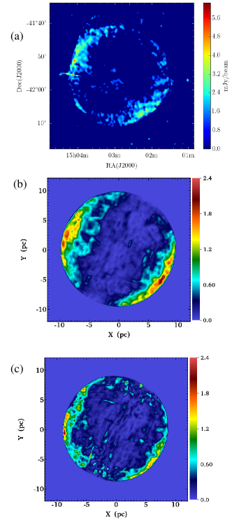
Figure 1: Comparison of the linearly polarized intensity at 1.4 GHz between the observations (panel (a)) and synthetic maps of a SNR expanding into a turbulent medium with adiabatic index $\gamma=5/3$ (model R1b, panel (b)) and $\gamma=1.3$ (model R2b, panel(c))

The numerical model employed is basically the same as in Schneiter et al. (2010, 2015), with the additional assumption of a turbulent background, where both the density and magnetic fluctuations have a 3D Kolmogorov-like power spectrum, as will be explained further down.

To simulate the evolution of SN 1006 we employed the Mezcal code (De Colle & Raga, 2006; De Colle et al., 2008; De Colle et al., 2012). This code solves the full set of ideal MHD equations in a Cartesian geometry with an adaptive mesh, and includes a cooling function to account for radiative losses (De Colle & Raga, 2006).

The computational domain is a cube of $24$ pc per side, which we will denote as ($x,y,z$), and is discretized on a five level binary grid with a maximum resolution of $4.7\times 10^{-2}$ pc. All the outer boundaries were set to outflow condition.

2.1 SNR initial conditions

In what follows, we describe the physical parameters and setup used to simulate the SNR, which are the same as those presented in Schneiter et al. (2015).

A supernova explosion is initialized by the deposition of $E_{0}=2.05\times 10^{51}$ erg in a radius of $R_{0}=0.65$ pc located at the centre of the computational domain. The energy is distributed such that $95\%$ of it is kinetic and the remaining $5\%$ is thermal.

The ejected mass was distributed in two parts: an inner homogeneous sphere of radius $r_{c}$ containing $4/7$ths of the total mass (M${}_{*}=1.4$M_⊙) with a density $\rho_{c}$, and an outer shell containing the remaining $3/7$ths of the mass following a power law ($\rho\propto r^{-7}$) as in Jun & Norman (1996a). The velocity has a increasing linear profile with $r$, which reaches a value of $v_{0}$ at $r=R_{0}$. The parameters $\rho_{c}$, $r_{c}$, and $v_{0}$ are functions of $E_{0}$, $M_{*}$, and $R_{0}$, and were computed using equations (1)-(3) of Jun & Norman (1996a).

2.2 The turbulent background

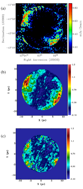
Figure 2: Same as Figure 1 but for maps of the Stokes parameter Q.

Jun & Jones (1999) suggested that the turbulent structures of the brightest radio emission correlate well with the magnetic field in general. For this reason we performed new simulations with a more realistic magnetized turbulent interstellar medium. In what follows, we will make use of equations (10) to (15) of Yu et al. (2015), which we reproduce below. To introduce the turbulent background we assumed a 3D Kolgomorov-like power spectrum fluctuation for both the density and the magnetic field, similar to that of Jokipii (1987) (see also Yu et al., 2015; Fang et al., 2014). The power spectrum follows:

$$P\propto\frac{1}{1+(kL_{c})^{11/3}}.$$ (1)

To generate the turbulence we assume a coherence length of $L_{c}=3\,pc$ and a wavenumber $k=\frac{2\pi}{L}$. Our simulations are computed with $N_{m}=903$ wave modes, and $L$ varies between $L_{min}=\Delta x$ and $L_{max}=L_{sim}$, being $\Delta x$ and $L_{sim}$ the cell and the computational domain sizes, respectively.

The initial magnetic field is given by:

$${\bf B}(x,y,z)={\bf B}_{0}+{\bf\delta B},$$ (2)

where ${\bf B_{0}}=B_{0}(x)\hat{y}$ and the magnetic field perturbation is:

$${\bf\delta B}=\Re\bigg{[}\sum_{n=1}^{N_{m}}A(k_{n})\left(\cos\alpha_{n}\hat{x}^{\prime}+i\sin\alpha_{n}\hat{y}^{\prime}\right)\exp(ik_{n}z_{n}^{\prime})\bigg{]},$$ (3)

with

$$A^{2}(k_{n})=\sigma_{B}^{2}\frac{\Delta V_{n}}{1+(k_{n}L_{c})^{11/3}}\sum_{n=1}^{N_{m}}\left[\frac{\Delta V_{n}}{1+(k_{n}L_{c})^{11/3}}\right]^{-1},$$ (4)

where $\sigma^{2}_{B}$ is the wave variance of the magnetic field, and the normalization factor, $\Delta V_{n}$, is given by:

$$\Delta V_{n}=4\pi k_{n}^{2}\Delta k_{n}.$$ (5)

Both systems $(x^{\prime},y^{\prime},z^{\prime})$ and $(x,y,z)$ are related by:

$$\begin{pmatrix}x^{\prime}\\ y^{\prime}\\ z^{\prime}\end{pmatrix}=\begin{pmatrix}\cos\theta_{n}\cos\phi_{n}&\cos\theta_{n}\sin\phi_{n}&-\sin\theta_{n}\\ -\sin\phi_{n}&\cos\phi_{n}&0\\ \sin\theta_{n}\cos\phi_{n}&\sin\theta_{n}\sin\phi_{n}&\cos\theta_{n}\end{pmatrix}\begin{pmatrix}x\\ y\\ z\end{pmatrix}$$

where $\theta_{n}$ and $\phi_{n}$ represent the direction of propagation of the wave mode $n$ with the wave number $k_{n}$ and polarization $\alpha_{n}$.

For the density fluctuation we employed the same log-normal distribution as in Giacalone & Jokipii (2007):

$$n(x,y,z)=n_{0}\exp({f_{0}+\delta f}),$$ (6)

where $f_{0}$ is a constant and $\delta f$ is the density perturbation with a wave variance $\sigma^{2}_{d}$. Both $\delta f$ and $\bf{\delta B}$ have the same 3D Kolmogorov-like power spectral index.

The turbulent environment temperature and number density were set to T${}_{0}=10^{4}$K and $n_{0}=5\times 10^{-2}$cm^-3, respectively. The wave variances for magnetic field and density were set as $\sigma^{2}_{B}=0.25\,B_{0}^{2}$ and $\sigma^{2}_{d}=0.4n_{0}^{2}$.

As mentioned above, one of the purposes of this work is to be able to study the effect of a perturbation on some observed parameters. To compare with the observations, the synthetic maps were performed for an integration time corresponding to $1000$ yr (the age of SN 1006).

3 Synthetic emission maps

Figure 3: Synthetic polar-referenced angle maps obtained from numerical simulations of the SNR 1006 expanding into a turbulent medium and with adiabatic index $\gamma=5/3$ (model R1b, panel (a)) and $\gamma=1.3$ (model R2b, panel(b)) The axes are in pc and the linear color scale is given in degrees.

run	$\gamma$	$\delta$B	$\delta\rho$
R1a	$5/3$	no	no
R1b	$5/3$	yes	yes
R2a	$1.3$	no	no
R2b	$1.3$	yes	yes
R2c	$1.3$	yes	no
R2d	$1.3$	no	yes

Table 1: Runs carried out in this paper with their corresponding hypothesis: adiabatic index, turbulent magnetic field and/or turbulent density distribution.

In Table 1 we list the runs that were carried out. With these runs we want to analyze the effects of both the reduction of the value of the adiabatic index $\gamma$ and/or the inclusion of a turbulent background with a Kolgomorov-like power spectrum for both density and magnetic field. These runs are labeled as R$i$p, where $i$ is 1 for the case of simulations with an adiabatic index $\gamma=5/3$, and 2 for $\gamma=1.3$. The label “p” indicates the presence or absence of turbulence in the background magnetic field and density: p = a indicates no turbulence in either variable; p = b includes turbulence in both; p = c only considers a turbulent $\bf B$; and p = d only considers a turbulent $\rho$.

Synthetic radio emission maps were obtained from the numerical results. In order to compare them with the observations, the computational domain (denoted as $xyz$ system), they were rotated with respect to the “image” system ($x_{i}y_{i}z_{i}$ system). At the beginning both systems coincide. The $x_{i}y_{i}$ plane of the “image” system is the plane of the sky, being $\hat{y}_{i}$ the direction towards the “North”, $-\hat{x}_{i}$ the direction towards the “East”, and the line of sight (hereafter LoS) the $\hat{z}$ direction. Then, synthetic maps were obtained after performing three rotations on the computational domain. First, a rotation around $\hat{y}_{i}$ was applied (the “North”) with an angle $\varphi_{y_{i}}$. Second, a rotation in $\varphi_{x_{i}}$ was carried out around the $\hat{x}_{i}$-direction. Finally, the computational domain was rotated by $\varphi_{z_{i}}$ around the $\hat{z}_{i}$-direction (the line of sight). To get the best agreement with the observations, after several tests these angles were set as $-15\degr$, $-30\degr$, and $60\degr$ for $\varphi_{x_{i}}$, $\varphi_{y_{i}}$, and $\varphi_{z_{i}}$, respectively . In this way, the projection of the unperturbed magnetic field ${\bf B_{0}}$ was tilted by $60\degr$ with respect to the $\hat{y}_{i}$ direction.

3.1 Synchrotron emissivity

For each point $(x_{i},y_{i},z_{i})$ of the SNR we can obtain the synchrotron specific intensity as (see Cécere et al., 2016, and references therein):

$$j(x_{i},y_{i},z_{i},\nu)\propto K\rho\ v^{4\alpha}\ B_{\perp}^{\alpha+1}\nu^{-\alpha},$$ (7)

where $\nu$ is the observed frequency, $B_{\perp}$ is the component of the magnetic field perpendicular to the LoS, $\alpha$ is the spectral index -which was set to $0.6$ for this object- and $\rho$ and $v$ are the density and velocity of the gas, respectively. The coefficient $K$ includes the obliquity dependence, being either proportional to $\sin^{2}{\Theta_{Bs}}$ for the quasi-perpendicular case or to $\cos^{2}{\Theta_{Bs}}$ for the quasi-parallel case. The angle $\Theta_{Bs}$ is the angle between the shock normal and the post-shock magnetic field (Fulbright & Reynolds, 1990). For the case of SN 1006, Bocchino et al. (2011) and Reynoso et al. (2013) showed that the observed morphology of this remnant can be explained by considering the quasi-parallel case. Schneiter et al. (2015) carried out a polarisation study of this remnant, based on 3D MHD simulations, finding that only the quasi-parallel case can succesfully reproduced the observed morpholoy of the Stokes parameter Q (see Figure 3 of Schneiter et al., 2015). For these reasons only the quasi-parallel case was considered in this work. The synthetic synchrotron emission maps are obtained by integrating $j(x_{i},y_{i},z_{i},\nu)$ along the LoS or $z_{i}$-axis, i.e.:

$$I(x_{i},y_{i},\nu)=\int_{\mathrm{LoS}}j(x_{i},y_{i},z_{i},\nu)dz_{i},$$ (8)

being $x_{i}$ and $y_{i}$ the coordinates in the plane of the sky.

3.2 Stokes parameters and position angle distribution maps

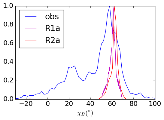
Figure 4: Comparison of the normalized distributions (with respect to their maxima) of the magnetic field position-angle as obtained from the observations and from the runs R1a and R2a (different $\gamma$ and both corresponding to a SNR propagating into a uniform medium, i.e. with $\delta$B = $\delta\rho=0$; see table 1), applying the polar-referenced angle selection.

With the purpose of comparing the numerical results with the observations, synthetic maps of the Stokes parameters $Q$ and $U$ were calculated as follows (Clarke et al., 1989; Jun & Norman, 1996b; Schneiter et al., 2015):

$$Q(x_{i},y_{i},\nu)=\int_{\mathrm{LoS}}f_{0}j(x_{i},y_{i},z_{i},\nu)\cos\left[2\phi(x_{i},y_{i},z_{i})\right]dz_{i},$$ (9)

$$U(x_{i},y_{i},\nu)=\int_{\mathrm{LoS}}f_{0}j(x_{i},y_{i},z_{i},\nu)\sin\left[2\phi(x_{i},y_{i},z_{i})\right]dz_{i},$$ (10)

where $\phi(x_{i},y_{i},z_{i})$ is the position angle of the local electric field in the plane of the sky and $f_{0}$ is the degree of linear polarization, which is a function of the spectral index $\alpha$:

$$f_{0}=\frac{\alpha+1}{\alpha+5/3}.$$ (11)

The position angle of the local magnetic field $\phi_{\mathrm{B}}(x_{i},y_{i},z_{i})$ is known from the simulations, and the position angle of the local electric field $\phi(x_{i},y_{i},z_{i})$ can be obtained from $\phi_{\mathrm{B}}(x_{i},y_{i},z_{i})$ by applying a $\frac{\pi}{2}$ rotation and correcting for Faraday rotation, as:

$$\phi(x_{i},y_{i},z_{i})=\phi_{\mathrm{B}}(x_{i},y_{i},z_{i})-\frac{\pi}{2}+\Delta\chi_{\mathrm{F}}.$$ (12)

The Faraday correction term $\Delta\chi_{\mathrm{F}}$ is given by:

$$\Delta\chi_{\mathrm{F}}=\mathrm{RM}\ \lambda^{2},$$ (13)

where RM is the rotation measure (in units of $\mathrm{rad\ m^{-2}}$) and $\lambda$ is the wavelength of the observations (given in m). In the present study, only the external RM arising in the foreground ISM is considered. Bandiera & Petruk (2016) explored the effects of internal RM on the polarized synchrotron emission of SNRs. For the case of SN 1006, we have carried out a rough estimation of the internal RM, obtaining a value close to 10% of the reported one by Reynoso et al. (2013) who obtained a RM of 12 $\mathrm{rad\ m^{-2}}$ for this remnant.

The linearly polarized intensity is computed as:

$$I_{P}(x_{i},y_{i},\nu)=\sqrt{Q(x_{i},y_{i},\nu)^{2}+U(x_{i},y_{i},\nu)^{2}}$$ (14)

and the maps of the polarization angle distribution were computed as follows:

$$\chi(x_{i},y_{i})=\frac{1}{2}\tan^{-1}(U(x_{i},y_{i},\nu)/Q(x_{i},y_{i},\nu))$$ (15)

Similarly, the distribution of the magnetic field orientation can be calculated as:

$$\chi_{\mathrm{B}}(x_{i},y_{i})=\frac{1}{2}\tan^{-1}(U_{\mathrm{B}}(x_{i},y_{i},\nu)/Q_{\mathrm{B}}(x_{i},y_{i},\nu))$$ (16)

where $U_{\mathrm{B}}(x_{i},y_{i},\nu)$ and $Q_{\mathrm{B}}(x_{i},y_{i},\nu))$ are calculated with the equations (9) and (10) and replacing $\phi(x_{i},y_{i},\nu)$ with $\phi_{\mathrm{B}}(x_{i},y_{i},\nu)$.

4 Results

4.1 Synthetic polarization maps

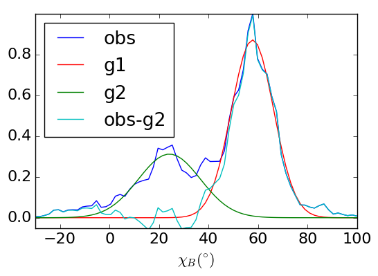
Figure 5: Two Gaussian fit of the observed position-angle distribution.

Figure 1 shows a comparison between the observed map of the linearly polarized intensity of SN 1006 (upper panel), and the synthetic polarization maps obtained for runs with $\gamma=5/3$ (run R1b, middle panel) and $\gamma=1.3$ (run R2b, bottom panel) by using Equation (14). The observed map was constructed by combining data obtained with the ATCA and the VLA at 1.4 GHz, as explained in Reynoso et al. (2013). The polarized emission image, as well as the distribution of the Q and U parameters, were convolved to a $15^{\prime\prime}$ beam. The two models used to construct the synthetic maps consider that the SNR is expanding into a turbulent medium with perturbations in both density and magnetic field. These synthetic maps are shown in arbitrary units. Two opposite bright, noisy arcs are observed in both synthetic maps, having a striking resemblance to the observations. Reducing the value of $\gamma$ produces a 5% smaller expansion radius of the remnant as measured on the linearly polarized intensity maps.

Following the analysis developed by Schneiter et al. (2015), we compare the observational and synthetic maps of the Stokes parameter Q, obtained for the quasi-parallel case using Equation 9. These maps are shown in Figure 2. A good overall agreement between observations and numerical results is obtained, since the opposite bright arcs are well reproduced. Also, note that these arcs are slightly more elongated than the ones obtained for the non-turbulent ISM (Schneiter et al., 2015).

4.2 Polar-referenced angle and a statistical study

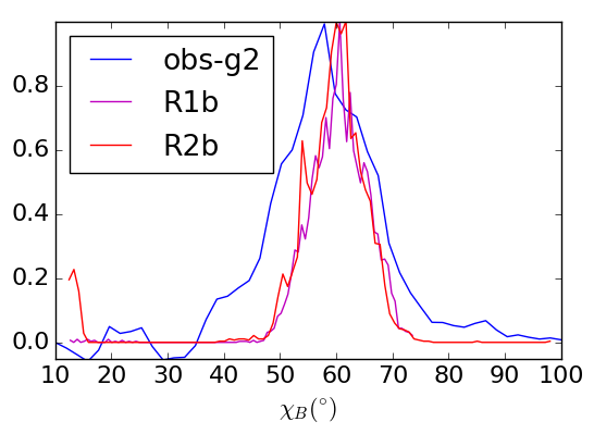
Figure 6: Same as Figure 4 but comparing the distribution obtained for observations (excluding the contribution of Gaussian g2) and runs R1b and R2b (with different $\gamma$ and for a turbulent medium, i.e. including both $\delta\rho$ and $\delta$B).

Gaussian	mean($\degr$)	$\sigma$($\degr$)
g1	$58.0$	$9.0$
g2	$23.0$	$13.0$

Table 2: Two Gaussian fit of the observational position-angle distribution

The polar-referenced angle distribution $\chi_{r}$ is given by:

$$\chi_{r}=\cos^{-1}(\hat{r}\cdot{\hat{b}}_{\perp}),$$ (17)

where $\hat{r}=(-x,y)/\sqrt{x^{2}+y^{2}}$ is the radial direction and $\hat{b}_{\perp}=(-sin(\chi_{\mathrm{B}}),cos(\chi_{\mathrm{B}}))$ is the direction of the magnetic field perpendicular to the LoS, which is obtained through Equation (16).

By using Equation (17), polar-referenced angle maps are obtained for runs R1b and R2b, which are shown in Figure 3. The blue color indicates the region where the magnetic field is almost parallel to the radial direction, while red color highlights the regions where it is mostly perpendicular.

Given that the polar-referenced angle technique is a useful tool for estimating the direction of the pre-shock ISM magnetic field (see Reynoso et al., 2013; Schneiter et al., 2015) we carried out a statistical study based on the analysis of the position-angle distribution in those regions where $\chi_{r}$ approaches zero.

The analysis was performed for both the numerical results and the observations in regions with synchrotron intensities larger than $10$% of the maximum, and where the condition $\chi_{r}\leq 14\degr$ (the observational angle error) is satisfied. These criteria were chosen to assure a good signal to noise ratio of the sample. The results are shown in Figure 4. To obtain the observational distribution, electric vectors were computed by combining the Q and U images with the miriad task IMPOL, and were later rotated by $\frac{\pi}{2}$ to convert them into magnetic vectors. The observational curve has two maxima: a large one at $\sim 57\degr$ and a small one at $\sim 25\degr$. Figure 5 shows a fitting of the observational distribution by two Gaussian labeled as g1 and g2, whose parameters are given in Table 2. The mean value of Gaussian g1 is 58°, which is close to the inclination of the Galactic plane (60°) and in agreement with the maxima of the curves computed for the runs R1a and R2a (see Figure 4).

It is reasonable to expect that the resulting ambient magnetic field is parallel to the Galactic plane at the latitude of SN 1006 (Bocchino et al., 2011; Reynoso et al., 2013; Schneiter et al., 2015). The secondary peak of the observed position-angle distribution would indicate an extra magnetic field component, which is not considered in our simulations. In order to eliminate this secondary unmodelled component, we subtracted the Gaussian fit labeled g2 from the observed distribution. The resulting curve will be referred to as the modified observational distribution.

Figure 6 compares the modified observational distribution with those resulting from the runs R1b and R2b. Clearly these numerical curves display now wider distributions compared with runs R1a and R2a, which is a consequence of including perturbations in B and $\rho$. The maxima of numerical distributions remain close to 60°.

In Figure 7 we explore the effect of selectively including the perturbations in $B$ and/or $\rho$ for $\gamma$ = 1.3. The curve corresponding to the run R2d ($\delta\rho\,\neq\,0$ and $\delta$B$\,=0$) does not show any significant widening, in contrast with those corresponding to the runs R2b and R2c, both with $\delta$B$\,\neq 0$. In order to carry out a more quantitative study, a statistical analysis was performed, comparing the distributions of the position-angle obtained from observations (subtracting the contribution of Gaussian g2) and simulations. The results of this statistical analysis are summarized in Table 3. Comparing the values obtained for the standard deviation, skewness and kurtosis, we note that the models achieving a better fit with the observations are those that consider a perturbed magnetic field, and a lower $\gamma$ (runs R2b and R2c).

	mean($\degr$)	$\sigma$($\degr$)	skewness	kurtosis
R1a	$60.$	$3.5$	$-0.32$	$0.2$
R1b	$59.$	$7.5$	$0.52$	$5.2$
R2a	$62.$	$6.6$	$-5.80$	$91.0$
R2b	$58.$	$11.0$	$-3.0$	$9.7$
R2c	$56.$	$13.0$	$-2.2$	$4.7$
R2d	$58.$	$9.9$	$-3.70$	$14.0$
obs-g2	$57.$	$22.0$	$-0.68$	$6.5$

Table 3: Statistics of the position-angle distributions

5 Discussion and conclusions

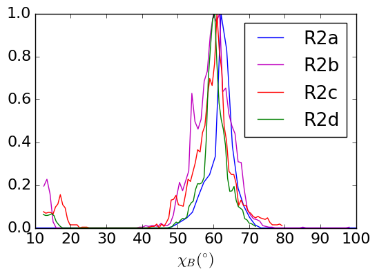
Figure 7: Comparison of the position-angle distributions obtained for runs R2p, i.e. those considering $\gamma=1.3$. In model R2a the medium is initialized as uniform at the beginning of the simulation, while in model R2b the SNR propagates into a turbulent medium (i.e., $\delta B,\delta\rho\neq 0$. In models R2c and R2d the medium is “partially” turbulent, with $\delta B\neq 0,\delta\rho=0$ and $\delta\rho\neq 0,\delta B=0$ respectively.

A radio polarization study of SN 1006 was performed based on 3D MHD simulations, considering the expansion of the remnant into a turbulent interstellar medium (including both magnetic field and density perturbations).

The inclusion of perturbations in magnetic field and density do not change the main conclusion of Schneiter et al. (2015), namely that the quasi-parallel case is the acceleration mechanism that better explains the observed morphology in the distribution of the Stokes parameter Q.

Based on the polar-referenced angle method, a study of the position angle distribution of the magnetic field was performed on both the observations and numerical results. This study reveals that the observational distribution is wide and has two maxima or components: a large one at 58°that coincides with the expected direction of the ambient magnetic field, and a small component at 23°. The curves corresponding to runs R1a an R2a have a single peak and narrower distributions. The secondary peak of the observations could be due to local blow-outs produced during the expansion of parts of the main SNR shock front into low-density cavities, such as those explored by Yu et al. (2015). Since our simulations do not have this secondary component we filtered it our from the observations and focused our comparison with the dominant component, as explained in the previous section.

The subsequent analysis was carried out by comparing the position-angle distributions obtained from numerical simulations with the observational distribution curve. A statistical study performed on these distributions reveals that models which include a turbulent pre-shock magnetic field, successfully explain the observed polar-angle distribution. Furthermore, all of them share a maximum at a position angle of 60$\degr$, which is parallel to the Galactic Plane and coincides with the expected direction of the Galactic magnetic field around SN1006 (Bocchino et al., 2011; Reynoso et al., 2013).

In summary, the statistical analysis based on the polar-referenced angle technique carried out in this work made it possible to recover the orientation of the ambient magnetic field. Based on previous observational and theoretical studies of SN1006 (Bocchino et al., 2011; Reynoso et al., 2013; Schneiter et al., 2015), we have only considered the quasi-parallel acceleration mechanism to estimate the synchrotron emission. However, it is important to mention that the same technique presented here can be applied with the quasi-perpendicular case. Finally, a good agreement between observations and numerical results is obtained if the simulations include magnetic field perturbations.

References

- Balsara et al. (2001) Balsara D., Benjamin R. A., Cox D. P., 2001, ApJ., 563, 800
- Bandiera & Petruk (2016) Bandiera R., Petruk O., 2016, MNRAS, 459, 178
- Bocchino et al. (2011) Bocchino F., Orlando S., Miceli M., Petruk O., 2011, A&A, 531, A129
- Cassam-Chenaï et al. (2008) Cassam-Chenaï G., Hughes J. P., Reynoso E. M., Badenes C., Moffett D., 2008, ApJ, 680, 1180
- Cécere et al. (2016) Cécere M., Velázquez P. F., Araudo A. T., De Colle F., Esquivel A., Carrasco-González C., Rodríguez L. F., 2016, ApJ, 816, 64
- Clarke et al. (1989) Clarke D. A., Burns J. O., Norman M. L., 1989, ApJ, 342, 700
- De Colle & Raga (2006) De Colle F., Raga A. C., 2006, A&A, 449, 1061
- De Colle et al. (2008) De Colle F., Raga A. C., Esquivel A., 2008, ApJ., 689, 302
- De Colle et al. (2012) De Colle F., Granot J., López-Cámara D., Ramirez-Ruiz E., 2012, ApJ., 746, 122
- Fang & Zhang (2012) Fang J., Zhang L., 2012, MNRAS, 424, 2811
- Fang et al. (2014) Fang J., Yu H., Zhang L., 2014, MNRAS, 445, 2484
- Fulbright & Reynolds (1990) Fulbright M. S., Reynolds S. P., 1990, ApJ, 357, 591
- Giacalone & Jokipii (2007) Giacalone J., Jokipii J. R., 2007, ApJL, 663, L41
- Guo et al. (2012) Guo F., Li S., Li H., Giacalone J., Jokipii J. R., Li D., 2012, ApJ., 747, 98
- Jokipii (1987) Jokipii J. R., 1987, ApJ, pp 842–846
- Jokipii et al. (1969) Jokipii J. R., Lerche I., Schommer R. A., 1969, ApJL, 157, L119
- Jun & Jones (1999) Jun B.-I., Jones T. W., 1999, ApJ, 511, 774
- Jun & Norman (1996a) Jun B.-I., Norman M. L., 1996a, ApJ, 465, 800
- Jun & Norman (1996b) Jun B.-I., Norman M. L., 1996b, ApJ, 472, 245
- Kesteven & Caswell (1987) Kesteven M. J., Caswell J. L., 1987, A&A, 183, 118
- Lee & Jokipii (1976) Lee L. C., Jokipii J. R., 1976, ApJ, 206, 735
- Reynoso et al. (2013) Reynoso E. M., Hughes J. P., Moffett D. A., 2013, AJ, 145, 104
- Schneiter et al. (2010) Schneiter E. M., Velázquez P. F., Reynoso E. M., de Colle F., 2010, MNRAS, 408, 430
- Schneiter et al. (2015) Schneiter E. M., Velázquez P. F., Reynoso E. M., Esquivel A., De Colle F., 2015, MNRAS, 449, 88
- West et al. (2016a) West J. L., Safi-Harb S., Ferrand G., 2016a, preprint, (arXiv:1609.02887)
- West et al. (2016b) West J. L., Safi-Harb S., Jaffe T., Kothes R., Landecker T. L., Foster T., 2016b, A&~A, 587, A148
- Yu et al. (2015) Yu H., Fang J., Zhang P. F., Zhang L., 2015, A&A, 579, A35