Modelling of Lyman-alpha Emitting Galaxies and Ionized Bubbles at the Era of Reionization

Abstract

Understanding $\rm{Ly{\alpha}}$ emitting galaxies (LAEs) can be a key to reveal cosmic reionization and galaxy formation in the early Universe. Based on halo merger trees and $\rm{Ly{\alpha}}$ radiation transfer calculations, we model redshift evolution of LAEs and their observational properties at $z\geq 6$. We consider ionized bubbles associated with individual LAEs and IGM transmission of $\rm{Ly{\alpha}}$ photons. We find that $\rm{Ly{\alpha}}$ luminosity tightly correlates with halo mass and stellar mass, while the relation with star formation rate has a large dispersion. Comparing our models with the observed luminosity function by Konno et al., we suggest that LAEs at $z\sim 7$ have galactic wind of $V_{\rm out}\gtrsim 100~{}\rm km\,s^{-1}$ and Hi column density of $N_{\rm HI}\gtrsim 10^{20}~{}\rm cm^{-2}$. Number density of bright LAEs rapidly decreases as redshift increases, due to both lower star formation rate and smaller Hii bubbles. Our model predicts future wide deep surveys with next generation telescopes, such as JWST, E-ELT and TMT, can detect LAEs at $z\sim 10$ with a number density of $n_{\rm LAE}\sim{\rm a~{}few~{}}\times 10^{-6}~{}\rm Mpc^{-3}$ for the flux sensitivity of $10^{-18}~{}\rm erg\,cm^{-2}\,s^{-1}$. By combining these surveys with future 21-cm observations, it could be possible to detect both LAEs with $L_{\rm Ly\alpha}\gtrsim 10^{42}~{}\rm erg~{}s^{-1}$ and their associated giant Hii bubbles with the size $\gtrsim 250~{}\rm kpc$ at $z\sim 10$.

1 Introduction

One of the major challenges in today’s astronomy is revealing cosmic reionization history with galaxy evolution. Recent CMB observations suggested cosmic reionization occurred at $z\sim 8-11$ (Komatsu et al. 2011; Planck Collaboration et al. 2014, 2016). Gunn-Peterson tests by the observations of high-redshift QSOs indicated cosmic reionization completed at $z\sim 6$ (e.g., Fan et al. 2006). However, the ionization history of integer-galactic medium (IGM) has not been understood yet. Recent observations of high-redshift galaxies at $z\gtrsim 7$ are gradually unveiling the cosmic star formation history (Ouchi et al. 2010; Bouwens et al. 2012, 2015; Oesch et al. 2015, 2016), and have allowed us to speculate the cosmic reionization history (Robertson et al. 2015). Yet, even considering the above observational constraints, various reionization histories remain viable (Cen 2003; Yajima & Khochfar 2015). One of the main uncertainties is low-mass galaxy formation with the halo mass $M_{\rm h}$ less than $\sim 10^{12}~{}\rm{M_{\odot}}$. Due to their higher number density and the higher escape fraction of ionizing photons from them (Razoumov & Sommer-Larsen 2010; Paardekooper et al. 2013; Yajima et al. 2011, 2014), low-mass galaxies can be responsible for main ionizing sources. However, the detection sensitivities of current observations are not sufficient to constrain the formation of low-mass galaxies. Therefore it is important to theoretically investigate the formation of low-mass galaxies and their contribution to cosmic reionization.

Most of high-redshift low-mass galaxies are observed as $\rm{Ly{\alpha}}$ emitters (LAEs; Hu & McMahon 1996; Steidel et al. 2000; Iye et al. 2006; Gronwall et al. 2007; Ouchi et al. 2008, 2010; Bond et al. 2011; Ciardullo et al. 2012; Yamada et al. 2012). Ouchi et al. (2010) indicated that LAEs were hosted in halos with the halo mass $M_{\rm h}\sim 10^{11}~{}\rm{M_{\odot}}$ by the clustering analysis (see also, Gawiser et al. 2007). Verhamme et al. (2008) suggested that LAEs were not dust-enriched well yet so that $\rm{Ly{\alpha}}$ photons escaped from galaxies against dust attenuation (see also, Yajima et al. 2014). These suggest LAEs are likely to be in the early phase of galaxy evolution (e.g., Mori & Umemura 2006). In addition, LAEs are one of major populations of galaxies contributing to the cosmic star-formation rate density in the early Universe (Ciardullo et al. 2012).

LAEs also have been used as a tool to investigate the early Universe (Iye et al. 2006; Vanzella et al. 2011; Ono et al. 2012; Shibuya et al. 2012; Finkelstein et al. 2013; Zitrin et al. 2015; Song et al. 2016b). Number density of LAEs rapidly decreases at $z\gtrsim 7$ (Ono et al. 2012; Konno et al. 2014), indicating that $\rm{Ly{\alpha}}$ fluxes from some galaxies were significantly attenuated due to neutral hydrogen in the IGM (e.g., Kashikawa et al. 2006). Meanwhile, LAEs themselves could provide sufficient ionizing photons into the IGM (Yajima et al. 2009, 2014), and some of them could make giant Hii bubbles that allowed $\rm{Ly{\alpha}}$ photons to reach us. In this case, galaxies can be observed as LAEs. In practice, the most distant LAE has been observed even at $z=8.68$ (Zitrin et al. 2015). Thus, LAEs can be the key objects in understanding the galaxy formation and cosmic reionization.

In this work, we investigate the evolution of LAEs with their associated Hii bubbles. By modeling both LAEs and Hii bubbles simultaneously, we estimate $\rm{Ly{\alpha}}$ luminosity functions (LFs), number density of LAEs, size distribution of Hii bubbles, and the relation between $\rm{Ly{\alpha}}$ flux and the size of Hii bubble. These estimations are useful for future observational missions. James Webb Space Telescope (JWST) is going to be launched at 2018, and aims to observe galaxies at $z\sim 10$. Its high sensitivity of spectroscopy will make it possible to detect $\rm{Ly{\alpha}}$ flux from galaxies if they distribute in giant Hii bubbles. Later on, 30-m class ground telescopes, the European Extremely Large Telescope (E-ELT), the Thirty Meter Telescope (TMT), and the Giant Magellan Telescope (GMT), will investigate galaxies at $z\sim 10$ statistically. In addition, several 21-cm observational missions are on going, e.g., the LOw Frequency ARray (LOFAR; Harker et al. 2010), and Murchison Widefield Array (MWA; Lonsdale et al. 2009). In future, Square Kilometer Array phase-2 (SKA-2; Dewdney et al. 2009) will perform large-scale 21-cm tomography. Since 21-cm emission comes from Hi gas, detections of holes of 21-cm signal indicate giant Hii bubbles around galaxies. Therefore, a combination of 21-cm and galaxy observations will provide fruitful information about the cosmic reionization and galaxy formation (e.g., Lidz et al. 2009).

Theoretically large-scale simulations showed that galaxies made patchy ionization structures in an inside-out fashion (e.g., Iliev et al. 2006, 2012; Mellema et al. 2006; Trac & Cen 2007; Ocvirk et al. 2016), whereas low-density void regions would be ionized first, in the so-called outside-in fashion, if AGNs were the main ionizing sources. However, AGNs are unlikely to be main ionizing sources because of the rapid decrease of observed number density at redshift $z>4$ (e.g., Richards et al. 2006), although the contribution of faint AGNs is still under the debate (Madau & Haardt 2015; Yoshiura et al. 2016; Khaire et al. 2016). Thus, in this paper, we model LAEs assuming the reionization model with the inside-out fashion. In order to understand cosmic reionization theoretically, we need high spatial resolution to follow the detailed physical processes of interstellar medium, as well as large volume to consider large-scale inhomogeneity of ionization structure. Even current numerical simulations cannot resolve such a wide dynamic range. For that reason, in this work, we semi-analytically investigate the cosmic reionization and galaxy formation based on simple structure formation models and radiative transfer calculations.

The distributions of LAEs at $z>6$ can provide us valuable information about cosmic reionization and galaxy formation (e.g., see the review by Dijkstra 2014). Furlanetto et al. (2004) investigated the IGM damping wing absorption of $\rm{Ly{\alpha}}$ flux from star-forming galaxies, and suggested that the $\rm{Ly{\alpha}}$ line could be a tool to investigate neutral fraction of IGM. McQuinn et al. (2007a) calculated the large-scale inhomogeneous ionization structure of IGM by combining $N$-body simulations with post-processing radiation transfer calculations. They calculated the spatial distribution of LAEs after IGM transmission using simple line profiles of gaussian or single frequency with velocity offset, and showed that the neutral IGM significantly changed the distribution of LAEs (see also, Mesinger et al. 2015). Numerical modeling of large-scale IGM ionization structure always suffers from the expensive calculation cost of radiation transfer. Therefore, Mesinger & Furlanetto (2008) developed a semi-numerical method to calculate the ionization structure of IGM, and investigated reionization structures with the volume of $(250~{}\rm Mpc)^{3}$ in comoving unit. This semi-numerical method significantly reduces the calculation amount, but simulates the ionization structure accurately (Zahn et al. 2011).

These previous works investigated the impacts of neutral IGM on the distributions of LAEs with detailed calculations of the IGM ionization structure. In this work, we focus on the following two points: (1) What are physical properties of observable LAEs at $z\gtrsim 7$?, (2) Can LAEs be observed even at $z\gtrsim 10$? We investigate these points statistically based on a large galaxy sample and $\rm{Ly{\alpha}}$ line profile models with a wide range of galactic inflow/outflow velocities, which have not been understood well in previous studies. The IGM transmission sensitively depends on the line profiles that are related with physical properties of gas in galaxies, e.g., velocity field, Hi column density (Dijkstra et al. 2006; Verhamme et al. 2006; Laursen et al. 2009; Yajima et al. 2012b). Some previous works showed the impacts of neutral IGM on the line profiles. Using the semi-numerical method, Dijkstra et al. (2011) calculated the IGM transmission to $\rm{Ly{\alpha}}$ flux from a galaxy with $M_{\rm h}\sim 10^{10}~{}\rm{M_{\odot}}$ at $z=8.6$, and suggested such a galaxy could be observed even when IGM was not fully ionized. They assumed that the galaxy had an expanding gas shell with the outflow velocity of $200~{}\rm km~{}s^{-1}$. Mesinger et al. (2015) investigated the redshift evolution of LAEs fraction in Lyman break galaxies (LBGs) by combining the large-scale ionization structures calculated by the semi-analytical models and simple Gaussian line profiles with the velocity offset $\Delta v=0,200$ and $400~{}\rm km~{}s^{-1}$. Choudhury et al. (2015) also used a Gaussian profile with a velocity offset depending on the redshift, $\Delta v=100[(1+z)/7]^{-3}~{}\rm km~{}s^{-1}$, and estimated the $\rm{Ly{\alpha}}$ equivalent width distributions to reproduce the observations. Thus most previous works have used simplified models for the line profiles, while the ionization structures have calculated in detail by numerical simulations. Meanwhile, Jensen et al. (2013) estimated outflow velocities from hydrodynamics simulations, and claimed the cosmic reionization rapidly completed at redshifts between $z\sim 6$ and $\sim 7$. However, it is generally difficult to accurately model galactic outflow even with state-of-the-art hydrodynamics simulations because the limited numerical resolution does not allow us to determine the strength of supernova feedback. Therefore, as a complementary work to previous works, here we investigate the physical properties of LAEs, in particular, the typical outflow/inflow velocity by using wide-range velocity parameter sets from $-300$ to $300~{}\rm km~{}s^{-1}$. Moreover, in simulating intrinsic $\rm{Ly{\alpha}}$ line profiles, we utilize two spherical symmetric gas models: (1) expanding uniform clouds, (2) expanding shells.

In addition, we make relations among $\rm{Ly{\alpha}}$ luminosities, sizes of Hii bubbles, star formation rates, and stellar masses. Recent observations have detected some distant galaxy candidates at $z\gtrsim 8$ by the LBG selection (e.g., Oesch et al. 2015, 2016). They showed the stellar mass and star formation rates of the candidates by SED fittings. Therefore, the relations between $\rm{Ly{\alpha}}$ luminosity and the physical properties can be a powerful tool to find out the objects which are likely to emit the $\rm{Ly{\alpha}}$ flux for future deep spectroscopy observations.

Then, using modeled LAEs, we also study observability of LAEs at $z\gtrsim 10$ by next generation telescope, e.g., JWST. The detection of emission lines from distant galaxies is quite important to determine the redshift and confirm the authenticity of candidates. Recent observations have allowed us to detect a distant LAE up to $z=8.68$ (Zitrin et al. 2015). However, as shown in recent LAEs observations (e.g., Ono et al. 2012), number density of LAEs rapidly decreases toward higher redshifts at $z\gtrsim 7$. This implies the difficulty of observations of LAEs at $z\gtrsim 7$ due to the IGM attenuation when the neutral fraction of the Universe is high. Therefore, it is important to study whether we can observe LAEs even at $z\gtrsim 10$ by JWST and other upcoming telescopes. We will show number densities of observable LAEs at $z\gtrsim 10$ based on simple expanding gas shell/cloud models.

In this work, we model star formation histories of galaxies based on halo merger histories, and ionized bubbles as expanding isolated ones associated with individual galaxies. Therefore, we do not consider expansion of ionized bubbles due to the overlap of them, i.e., we focus on field galaxies, not clustering galaxies that are likely to make the overlapped giant Hii bubbles. McQuinn et al. (2007b) presented cosmological simulations of different reionization scenarios with post-processing radiation transfer simulations. Depending on physical parameters, i.e., star formation efficiency and escape fraction of ionizing photons, various ionization structure and history can be considered under the same value of volume-weighted mean ionization fraction. They showed the overlaps of Hii regions were delayed in the model that assumed low-mass galaxies contributed to cosmic reionization significantly. In addition, recent CMB observation obtained the Thomson scattering optical depth of IGM $\tau_{\rm e}=0.058$, corresponding to the reionization redshift of $z_{\rm re}\sim 8.8$ under the assumption that all IGM were instantaneously ionized at $z_{\rm re}$. Since the Gunn-Peterson tests using QSOs indicated that the reionization was completed at $z\sim 6$ (e.g., Fan et al. 2006), Hii bubbles might not be overlapped well at $z\gtrsim 7$. Thus, in this work, we simply follow evolutions of isolated expanding Hii bubbles without the effect of overlap. With a simple prescription, we also discuss the effect of the overlap of Hii bubbles on the IGM transmission.

Tilvi et al. (2011) modeled LAEs at $z=3-7$ based on halo merger histories from cosmological $N$-body simulations. They assumed that $\rm{Ly{\alpha}}$ luminosity of each galaxy was simply proportional to SFR and all $\rm{Ly{\alpha}}$ photons escaped from galaxies, and all ionizing photons were absorbed by interstellar gas. On the other hand, in this work, we focus on LAEs at $z>6$, and consider non-zero escape fraction of ionizing photons to reproduce the observed Thomson scattering optical depth of IGM, and IGM transmission depending on $\rm{Ly{\alpha}}$ line profiles.

We use the cosmological parameters, $\Omega_{\Lambda}=0.7$, $\Omega_{\rm M}=0.3$, $\Omega_{\rm b}=0.045$ and $h=0.7$(Komatsu et al. 2011; Planck Collaboration et al. 2016).

The paper is organized as follows. We describe our models of star formation and Hii bubbles in §2. In §3, we present the results, which include the $\rm{Ly{\alpha}}$ properties, LFs of LAEs and redshift evolution of number density of LAEs. We discuss the relation between the $\rm{Ly{\alpha}}$ flux of galaxies and the sizes of Hii bubbles in §4, and summarize in §5.

2 Model

In the current standard picture of structure formation, halos grow via minor/major mergers. In our model, the star formation rate (SFR) in a halo is assumed to be proportional to the growth rate of the halo as follows:

$${\rm SFR}=\frac{dM_{\rm{star}}}{dt}=\frac{dM_{\rm{star}}}{dM_{\rm h}}\frac{dM_{\rm h}}{dt}.$$ (1)

The relation between stellar and halo mass can be written as $\frac{dM_{\rm{star}}}{dM_{\rm h}}=\frac{d{\rm log}M_{\rm{star}}}{d{\rm log}M_{\rm h}}\frac{M_{\rm{star}}}{M_{\rm h}}$. The abundance matching analysis by Behroozi et al. (2013) indicated that $\frac{d{\rm log}M_{\rm{star}}}{d{\rm log}M_{\rm h}}\sim{\rm const}$ for $M_{\rm h}\lesssim 10^{12}~{}\rm{M_{\odot}}$. In addition, Behroozi & Silk (2015) showed the weak dependence of $\frac{M_{\rm{star}}}{M_{\rm h}}$ on halo mass and redshift at the mass range $M_{\rm h}\sim 10^{11}-10^{13}~{}\rm{M_{\odot}}$, although $\frac{M_{\rm{star}}}{M_{\rm h}}$ increases with $M_{\rm h}$ at $M_{\rm h}\lesssim 10^{11}~{}\rm{M_{\odot}}$ (see also, Moster et al. 2013; Kravtsov et al. 2014). Therefore we here assume $\frac{dM_{\rm{star}}}{dM_{\rm h}}\sim{\rm const}$. Thus, we estimate SFR from the growth rate of halo mass with a constant tuning parameter $\alpha$, i.e., ${\rm SFR}=\alpha\frac{dM_{\rm h}}{dt}$.

In order to estimate the growth of halos, we use halo merger trees based on an extended Press-Schechter formalism (Somerville & Kolatt 1999; Khochfar & Burkert 2001, 2006). The halo merger trees include 5000 realizations with the halo mass range of $10^{9}-10^{13}~{}\rm{M_{\odot}}$ at $z=6$. In this work, we allow star formation only for halos with the mass $M_{\rm h}>10^{8}~{}\rm{M_{\odot}}$, because star formation in less massive halos can be significantly suppressed due to UV background or internal stellar feedback (e.g., Okamoto et al. 2008; Hasegawa & Semelin 2013). In deriving statistical properties, e.g., cosmic SFR density, stellar mass density and LF, we sum the contribution of each merger tree with normalization factors that reproduce the halo mass function of Sheth & Tormen (2002). We determine the tuning parameter by using observed cosmic SFR density and stellar mass density at $z\sim 7-8$. Figure 1 shows our modeled SFR and stellar mass density with observations. We choose the parameter $\alpha$ by the least square fitting to the four points of the observations. The observed SFR and stellar mass densities consider only galaxies with $M_{\rm UV}<-17$ and $M_{\rm{star}}\geq 10^{8}~{}\rm{M_{\odot}}$, respectively. Therefore, we consider only the galaxies satisfying the above criteria for the fitting. The best fit value is $\alpha=3.3\times 10^{-3}$. Note that, so far there is no available data about $\frac{dM_{\rm{star}}}{dM_{\rm h}}$ at $z\gtrsim 9$ and $\alpha$ can change with halo mass and redshift. However, for simplicity, we assume $\alpha$ is constant. Following the above way, we derive star formation history from each halo merger tree. Although we consider only bright galaxies in deriving the parameter $\alpha$ via the comparisons with the observations, we follow star formation of all halos with $M_{\rm h}\geq 10^{8}~{}\rm{M_{\odot}}$ in studying cosmic reionization and LAEs in this work. Black dash lines in the panels of Figure 1 represent the total SFR and stellar mass densities as a function of redshift. The top panel of Figure 1 shows that low-mass faint galaxies have non-negligible contribution to the cosmic SFR density and are expected to contribute to cosmic reionization as recent studies indicated (e.g., Yajima et al. 2009, 2011, 2014; Robertson et al. 2013; Cai et al. 2014; Wise et al. 2014).

We also derive UV LFs by converting SFR to UV flux with $L_{\rm\nu,UV}=0.7\times 10^{28}~{}{\rm erg~{}s^{-1}}~{}\left(\frac{\rm SFR}{\rm 1~{}\rm M_{\odot}~{}yr^{-1}}\right)$ (Madau et al. 1999). Figure 2 shows our modeled LFs at $z\sim 7$ and $\sim 8$ with those from the recent observation by Bouwens et al. (2015). The observation indicated that a part of UV flux are absorbed by dust with the escape fraction $f_{\rm esc,UV}\sim 0.6$. Our modeled LFs match the observation well with the same UV escape fraction.

Galaxies ionize the IGM as star formation proceeds. In a one-zone approximation, we estimate time evolution of cosmic ionization degree (Barkana & Loeb 2001),

$$\frac{dQ_{\rm HII}}{dt}=\frac{1}{n_{\rm H}^{0}}\dot{n}_{\rm ion}^{\gamma}f_{\rm esc,ion}-\alpha_{\rm B}C(1+z)^{3}n_{\rm H}^{0}Q_{\rm HII},$$ (2)

where $Q_{\rm HII}$ is the volume fraction of Hii, $n_{\rm H}^{0}$ is the present-day hydrogen number density ($\sim 2\times 10^{-7}~{}\rm cm^{-3}$), $\dot{n}_{\rm ion}^{\gamma}$ is the intrinsic ionizing photon emissivity per unit volume, $\alpha_{\rm B}$ is the case-B recombination rate, $C$ is a clumpiness factor of IGM, and $f_{\rm esc,ion}$ is escape fraction of ionizing photons, which is a free parameter here. We estimate $\dot{n}_{\rm ion}^{\gamma}$ from star formation history of each halo by using a population synthesis code starburst99 (Leitherer et al. 1999) with the Salpeter initial mass function with the metallicity of $10^{-2}~{}\rm Z_{\odot}$. The reionization history is shown in the upper panel of Figure 3. As $f_{\rm esc,ion}$ increases, the IGM is ionized earlier. We assume the recombination rate for $T=10^{4}~{}\rm K$ ($\alpha_{\rm B}=2.6\times 10^{-13}~{}\rm cm^{3}\;s^{-1}$) and $C=3$, as suggested by numerical simulations (Pawlik et al. 2009; Jeon et al. 2014).

The cosmic reionization history is regulated by $f_{\rm esc,ion}$. Free electrons produced by the cosmic reionization contribute to the Thomson scattering optical depth ($\tau_{\rm e}$) of CMB photons, defined as

$$\tau_{\rm e}=\int_{0}^{z_{\rm rec}}\sigma_{\rm T}n_{\rm e}(z)c\left|\frac{dt}{dz}\right|dz,$$ (3)

where $z_{\rm rec}=1100$ is the redshift at the time of recombination. In this work, we assume the single ionization fraction of helium is the same as the one for hydrogen at $z\geq 3$, and the double ionization takes place at $z<3$ (e.g., Wyithe et al. 2010; Inoue et al. 2013). Recent simulations show that indeed the fraction of Heii is close to the Hii fraction at high redshifts, although the ionization fraction of helium is slightly lower than the one for hydrogen (Ciardi et al. 2012). The top panel of Figure 3 represents the ionization history of hydrogen gas with the different $f_{\rm esc,ion}$. The bottom panel of Figure 3 shows $\tau_{\rm e}$ with different $f_{\rm esc,ion}$. The Thomson scattering optical depth $\tau_{\rm e}$ increases with redshift in a way depending on $f_{\rm esc,ion}$ due to the different ionization histories. We find $f_{\rm esc,ion}=0.2$ nicely reproduces the CMB observation (Planck 2016). Therefore, in this work, we adopt $f_{\rm esc,ion}=0.2$ with no redshift evolution. In fact, Yajima et al. (2014) showed $f_{\rm esc,ion}$ is constant with redshift and $\sim 0.2$ by cosmological simulations with radiative transfer calculations.

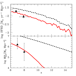
Figure 1: Upper panel: Star formation rate density. Red line represents our modeled star formation history based on the halo merger trees. Triangle symbols show the observation by Bouwens et al. (2015). The observed star formation rate densities are estimated by integrating the luminosity functions in the range of $M_{\rm UV}\leq-17$. Our model (red line) also consider only the galaxies brighter than the same limiting magnitude. Lower panel: Stellar mass density. Red line is the cumulated stellar mass of our model considering only the galaxies with $M_{\rm{star}}\geq 10^{8}~{}\rm{M_{\odot}}$. Triangle symbols show the observation by Song et al. (2016a), who integrated the derived stellar mass functions for galaxies with $M_{\rm{star}}\geq 10^{8}~{}\rm{M_{\odot}}$. Black dash lines represent the star formation rate and stellar mass densities considering all galaxies without the thresholds equivalent to the observations.

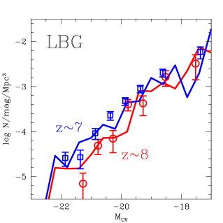
Figure 2: UV luminosity functions. Open squares and circles represent observed LBGs at $z\sim 7$ and $\sim 8$ by Bouwens et al. (2015).

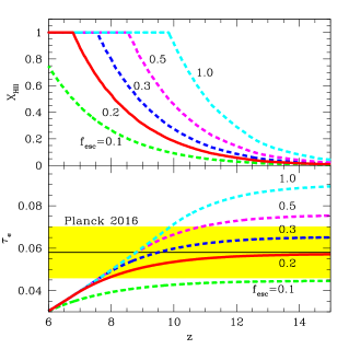
Figure 3: Upper panel: Ionization history. Different lines show ionization histories with different escape fractions of ionizing photons. Lower panel: Thomson scattering optical depth. Different lines are estimated with different ionization histories presented in the upper panel. Yellow shade represents the estimation by the CMB observation (Planck Collaboration et al. 2016).

3 Results

3.1 Evolution of ionized bubbles around galaxies

We follow the growth history of Hii bubbles around individual galaxies with the star formation efficiency $\alpha$ and $f_{\rm esc,ion}$ estimated above. Sizes of Hii bubbles evolve with ionizing photon emissions, recombination, and cosmic expansion as follows (Cen & Haiman 2000):

$$\frac{dR_{\rm HII}^{3}}{dt}=3H(z)R_{\rm HII}^{3}+\frac{3\dot{N}_{\rm ion}^{\gamma}f_{\rm esc,ion}}{4\pi n_{\rm H}(z)}-Cn_{\rm H}(z)\alpha_{\rm B}R_{\rm HII}^{3},$$ (4)

where $H(z)$ is the Hubble constant at specific redshifts, and $\dot{N}_{\rm ion}^{\gamma}$ is intrinsic ionizng photon emissivity of each galaxy. The ionizing fronts can propagate up to the Str$\rm\ddot{o}$mgren radius during the recombination time scale (Spitzer 1978). The recombination time scale is $t_{\rm rec}\sim\frac{1}{\alpha_{\rm B}n_{\rm H}}\sim 0.5~{}{\rm Gyr}~{}\left(\frac{1+z}{11}\right)^{-3}$, which is longer than the typical time scale over which SFR changes more than factor $\sim 2$. Therefore, Hii bubbles do not reach the equilibrium state, and we need to consider SFR history to estimate the sizes of Hii bubbles at given redshifts. We estimate probability distribution function (PDF) of the sizes of ionized bubbles ($R_{\rm HII}$) as shown in Figure 4. In our model, higher mass halos tend to possess larger ionized bubbles. Due to the decrease in the number density of halos on the high-mass end of a halo mass function (Sheth & Tormen 2002), the PDF of $R_{\rm HII}$ rapidly decreases at larger $R_{\rm HII}$. Although the ionizing front does not reach the size of Str$\rm\ddot{o}$mgren sphere $r_{\rm st}\propto(\dot{N}_{\rm ion}^{\gamma})^{1/3}(1+z)^{-2}$, it can be used as a rough indicator of sizes of Hii bubbles. As redshift decreases, the IGM density decreases while the number density of massive halos with higher ionizing photon emissivity increases. Therefore, the tail of PDF in the large-$R_{\rm HII}$ end shifts to larger $R_{\rm HII}$ at lower redshift. Future 21 cm observations, e.g., SKA-2, is supposed to probe the IGM ionization structure with the angular resolution of $\sim 1^{\prime}$. Therefore, at $z\lesssim 10$, the tail of PDF at large $R_{\rm HII}$ can be observationally investigated in future. The halo number density monotonically increases as the halo mass decreases at a fixed redshift. Since the size of Hii bubble is positively related with halo mass as will be shown in Section 3.3, it seems that the PDFs in the small-$R_{\rm HII}$ end monotonically increase as $R_{\rm HII}$ decreases. However, there are peaks in the PDFs, below which they decrease as $R_{\rm HII}$ decreases. This is caused by the threshold of halo mass for star formation imposed in this work.

Note that, in this work, we do not take the effect of overlap of Hii bubbles into account. The galaxy clustering causes the overlap of Hii bubbles that can extend the tails of PDFs to larger size. Since the overlapping effect can be larger as redshift decreases, the slopes of PDFs at lower redshifts can be changed to be more shallower. We will discuss the impacts of the overlap of Hii bubbles on luminosity functions in Section 3.2.

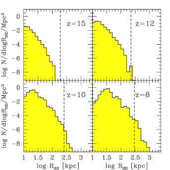
Figure 4: Probability distribution functions of sizes of Hii bubbles associated with individual galaxies. Vertical dash lines are corresponding to the viewing angle of 1 arcmin.

3.2 $\rm{Ly{\alpha}}$ luminosity functions

Absorption of ionizing photons by interstellar medium within galaxies results in $\rm{Ly{\alpha}}$ emissions via recombination processes, while escaped photons cause the cosmic reionization as shown in the previous section. The $\rm{Ly{\alpha}}$ luminosity ($L_{\rm Ly\alpha}$) is estimated by

$$L_{\rm Ly\alpha}=0.68(1.0-f_{\rm esc,ion})f_{\rm esc,Ly\alpha}\epsilon_{\rm{Ly{\alpha}}}\dot{N}_{\rm ion}^{\gamma},$$ (5)

where $f_{\rm esc,Ly\alpha}$ is the escape fraction of $\rm{Ly{\alpha}}$ photons from galaxies, $\epsilon_{\rm{Ly{\alpha}}}=10.2~{}\rm eV$ is the energy of a $\rm{Ly{\alpha}}$ photon. The escape fraction of $\rm{Ly{\alpha}}$ photons $f_{\rm esc,Ly\alpha}$ can be lower than $f_{\rm esc,UV}$ because the path length of $\rm{Ly{\alpha}}$ photons until escape can be longer due to multiple scattering process. However, if dust mainly distributes in Hi gas clumps, $f_{\rm esc,Ly\alpha}$ does not become lower than $f_{\rm esc,UV}$ because $\rm{Ly{\alpha}}$ photons are scattered by hydrogen on surface of the clumps before interacting with dust. Ciardullo et al. (2012) indicated that $f_{\rm esc,Ly\alpha}\sim f_{\rm esc,UV}$ for observed LAEs at $z\sim 2$. In addition, cosmological simulations of Yajima et al. (2014) showed that $f_{\rm esc,Ly\alpha}$ was $\gtrsim 0.6$ and similar to $f_{\rm esc,UV}$ at $z\gtrsim 6$. Therefore, in this work, we assume that $f_{\rm esc,Ly\alpha}=f_{\rm esc,UV}=0.6$.

Next, we estimate IGM transmission as a function of wavelength. As in Cen & Haiman (2000), we divide the paths along which $\rm{Ly{\alpha}}$ photons travel from galaxies to us into the two parts, i.e., outside and inside ionized bubbles, and separately estimate each contribution. The transmission outside ionized bubbles is estimated as follows:

$$\tau(\lambda_{\rm obs},z_{\rm s})=\int_{z_{\rm r}}^{z_{\rm i}}dz\,c\,\frac{dt}{dz}\,n_{\rm H}(z)x_{\rm HI}\sigma_{\rm{Ly{\alpha}}}\,[\lambda_{\rm obs}/(1+z)],$$ (6)

where $z_{\rm i}\sim z_{\rm s}-\frac{R_{\rm HII}\times(1+z)}{R_{\rm H}}$. Here, $z_{\rm r}$ is redshift when the cosmic reionization completes, which we set $z_{\rm r}=6$, $z_{\rm i}$ is redshift when $\rm{Ly{\alpha}}$ photons pass through ionizing front, $z_{\rm s}$ is redshift of galaxy, $\sigma_{\rm{Ly{\alpha}}}$ is the scattering cross section for Hi gas, and $R_{\rm H}$ is the size of the cosmological horizon at $z_{\rm s}$. We assume the outside of the bubble is completely neutral, i.e., $x_{\rm HI}=1$. The $\sigma_{\rm{Ly{\alpha}}}$ is estimated by (Verhamme et al. 2006)

$$\sigma_{\rm{Ly{\alpha}}}[\lambda]=1.041\times 10^{-13}\left(\frac{T}{10^{4}~{}\rm K}\right)^{-\frac{1}{2}}\frac{H(x,a)}{\sqrt{\pi}}.$$ (7)

We set $T=10^{4}~{}\rm K$ in this work. Here, $H(x,a)$ is the Voigt function,

$$H(x,a)=\frac{a}{\pi}\int_{-\infty}^{+\infty}\frac{e^{-y^{2}}}{(x-y)^{2}+a^{2}}dy$$ (8)

where $x\equiv(\nu-\nu_{0})/\Delta\nu_{\rm D}$, $\nu_{0}=2.466\times 10^{15}~{}\rm Hz$ is the line-center frequency, $\nu_{\rm D}$ is the Doppler width, $a=\Delta\nu_{\rm L}/(2\Delta\nu_{\rm D})$, $\Delta\nu_{\rm L}=9.936\times 10^{7}~{}\rm Hz$ is the natural line width. We here use the fitting formula of $H(x,a)$ given by Tasitsiomi (2006).

Even inside ionized bubbles, a tiny fraction of neutral hydrogens exist. We estimate the IGM transmission from ionizing front to virial radius with the neutral fraction under the ionization equilibrium state,

$$x_{\rm HI}=1.5\times 10^{-5}\left(\frac{C}{3}\right)\left(\frac{r}{\rm kpc}\right)^{2}\left(\frac{\dot{N}_{\rm ion}^{\gamma}}{10^{50}~{}\rm s^{-1}}\right)^{-1}\left(\frac{1+z}{8}\right)^{3}.$$ (9)

Note that, the optical depth outside the ionized bubble is dominant in our work. The IGM transmission is mostly almost zero at $\lambda\lesssim\lambda_{0}$, where $\lambda_{0}=1216~{}\rm\AA$ is the wavelength of $\rm{Ly{\alpha}}$ line center.

Considering the IGM transmission, we derive $\rm{Ly{\alpha}}$ LFs, and compare them with the observation of Konno et al. (2014). Depending on the shape of $\rm{Ly{\alpha}}$ line profile, the IGM transmission significantly changes. Even with recent deep spectroscopies, however, it is difficult to determine intrinsic $\rm{Ly{\alpha}}$ line profiles, i.e., before the IGM extinction (e.g., Ouchi et al. 2010). The intrinsic $\rm{Ly{\alpha}}$ line profile depends on the physical nature of galaxies, e.g., Hi column density and velocity field (e.g., Verhamme et al. 2006). In this work, we calculate intrinsic $\rm{Ly{\alpha}}$ line profiles by $\rm{Ly{\alpha}}$ radiation transfer simulations using the code developed in Yajima et al. (2012b), and study the physical nature of LAEs through the comparison with the observation (Konno et al. 2014). For the purpose, we employ the following two models for the internal velocity structure of a galaxy: (1) expanding cloud, (2) expanding shell. Both cloud and shell models have only two parameters: (1) Hi column density $N_{\rm HI}$, (2) outflow velocity $V_{\rm out}$. The intrinsic line profiles of the cloud model are calculated based on spherically outflowing gas with the following velocity structure,

$$V(r)=V_{\rm out}\left(\frac{r}{R_{\rm edge}}\right),$$ (10)

where $R_{\rm edge}$ is the edge of the spherical cloud and $V_{\rm out}$ is the outflow velocity at $R_{\rm edge}$. Here uniform gas density in the cloud is assumed. Although the simulated profiles do not depend on $R_{\rm edge}$, the source size is likely to increase with $R_{\rm edge}$. Since the surface brightness decreases with the source size, the detectability of $\rm{Ly{\alpha}}$ flux depends on the choice of $R_{\rm edge}$. Nevertheless, in this work, we assume that LAEs are compact and no flux is lost based on theoretical motivation: the typical sizes of galaxies become $\sim\lambda_{\rm spin}R_{\rm vir}$ (e.g., Mo et al. 1998) where $\lambda_{\rm spin}$ is a halo spin parameter and expected to be less than $\sim 0.1$ (e.g., Bullock et al. 2001). Therefore we consider $R_{\rm edge}=0.1R_{\rm vir}$ in which the source size may not be subject to the flux loss. The uncertainty of the surface brightness will be discussed in Sec. 4.4.

In the shell model, the velocity field is monochromatic, i.e.,

$$V(r)={\rm const.}=V_{\rm out}.$$ (11)

Our radiation transfer calculations are carried out in 100 spherical shells. All shells have same Hi density in the cloud model, while only most outside shell has Hi gas in the shell model.

The cloud and shell models approximate galactic outflows due to stellar feedback. When most of gas are being evacuated due to starburst, Hi gas structure may be close to the shell model. On the other hand, in the case of smooth star formation history, stars keep being formed in static Hi gas at near galactic centers, while a part of gas are evacuated from galaxies. In this case, the gas structure may be closer to the cloud model. The star formation and gas structure in high-redshift galaxies are still under the debate (e.g., Kimm & Cen 2014; Hopkins et al. 2014; Yajima et al. 2017). Therefore we here study LAEs by using these two models.

Figure 5 shows the modeled line profiles with various outflowing velocities. The $\rm{Ly{\alpha}}$ line profiles of the cloud model get the asymmetric shape with a peak at redder wavelength for the outflow velocity field, because $\rm{Ly{\alpha}}$ photons at bluer wavelength are scattered by Hi gas due to the Doppler shift. As $N_{\rm HI}$ increases, the line profiles are extended, and the peak frequency shift farther from the line center frequency. In the case of the shell model, the line profiles become more complicated because of the back scattering effect (Verhamme et al. 2006). Observable photons scattered by the shell at the far side from an observer make a bump at redder wavelength. In addition, when the Hi column density is low and the expanding velocity is large, most of $\rm{Ly{\alpha}}$ photons can directly escape from the shell, resulting in the peaks at the line center frequency as shown in middle and right panels of the shell model. For the inflow velocity field, the $\rm{Ly{\alpha}}$ line profile becomes the mirror symmetric shape to the one for outflow with the same absolute value of the velocity.

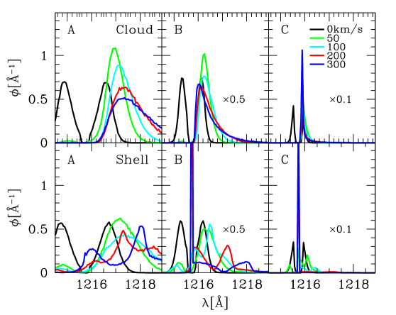
Figure 5: $\rm{Ly{\alpha}}$ line profiles from expanding spherical gas clouds or shells. Upper panels represent the line profiles of the cloud model that assume the velocity field as $V(r)=V_{\rm out}\left(\frac{r}{R_{\rm edge}}\right)$, where $R_{\rm edge}$ is the radius of clouds and $V_{\rm out}$ is the velocity at $R_{\rm edge}$. Lower panels present the line profiles of the shell model in which the velocity is constant, i.e., $V(r)=V_{\rm out}$. The different panels from left to right show the $\rm{Ly{\alpha}}$ profiles considering different Hi column densities: $N_{\rm HI}=2\times 10^{20}~{}\rm cm^{-2}$ (panel A), $2\times 10^{19}~{}\rm cm^{-2}$ (panel B), and $2\times 10^{18}~{}\rm cm^{-2}$ (panel C). The different lines represent the different expanding velocities at $R_{\rm edge}$. The $\phi(\lambda)$ is normalized to be unity when it is integrated over the wavelength. The $\phi(\lambda)$ of panel (B) and (C) is artificially reduced by a factor 2 and 10.

With the simulated intrinsic line profiles, we can estimate $\rm{Ly{\alpha}}$ LFs for given $N_{\rm HI}$ and $V_{\rm out}$. In this work, we infer typical $N_{\rm HI}$ and $V_{\rm out}$ of LAEs by comparing modeled LFs with the observed one by Konno et al. (2014). Figure 6 show the LFs. Here we calculate the LFs for three Hi column density models, $N_{\rm HI}=2\times 10^{20}~{}\rm cm^{-2}$ (model A), $N_{\rm HI}=2\times 10^{19}~{}\rm cm^{-2}$ (model B), and $N_{\rm HI}=2\times 10^{18}~{}\rm cm^{-2}$ (model C). The column density of model A is corresponding to Damped Lyman-$\alpha$ Systems (DLAs: Wolfe et al. 2005). Yajima et al. (2012a) showed that DLAs distributed at lines of sight passing star-forming regions in high-redshift star-forming galaxies by combining cosmological SPH simulations with radiation transfer calculations. These column densities are optically thick to ionizing photons, hence not consistent with $f_{\rm esc,ion}=0.2$. However, recent simulations showed ionizing photons mostly escape along ionized holes created by radiative and SNe feedback (e.g., Yajima et al. 2009, 2011; Kimm & Cen 2014). Thus, $f_{\rm esc,ion}$ of 20 $\%$ can be considered as the fraction of viewing angle along which star forming regions are not covered by Hi gas. For simplicity, we do not take account of the effect of such holes on line profiles. Note that, however, $\rm{Ly{\alpha}}$ line profiles somewhat change due to the holes, clumpiness or other detailed structure in Hi gas (Dijkstra & Kramer 2012).

The shaded regions in Figure 6 represent the LFs using different $\rm{Ly{\alpha}}$ line profiles with the velocity range from $V_{\rm out}=-300~{}\rm km~{}s^{-1}$ to $300~{}\rm km~{}s^{-1}$. The best fit velocities for the cloud model are $180~{}\rm\rm km\;s^{-1}$ (model A), $190~{}\rm\rm km\;s^{-1}$ (model B), and $110~{}\rm\rm km\;s^{-1}$ (model C), while in the case of the shell model they are $130~{}\rm\rm km\;s^{-1}$ (model A), $60~{}\rm\rm km\;s^{-1}$ (model B), and $40~{}\rm\rm km\;s^{-1}$ (model C), as summarized in Table 1. Only model A with the velocity range $V_{\rm out}\sim 100-300~{}\rm\rm km\;s^{-1}$ can reproduce the observed LF well. Therefore we suggest LAEs are likely to have high Hi column density with $\gtrsim 10^{20}~{}\rm cm^{-2}$ and outflowing Hi gas with velocity $\gtrsim 100~{}\rm km~{}s^{-1}$. These outflow velocities are consistent with recent observations of [Cii] emissions from LAEs at $z\sim 7$ in which they showed the velocity offsets between $\rm{Ly{\alpha}}$ and [Cii] lines (Pentericci et al. 2016). Note that, the cloud model has low velocity component at a galactic center, unlike the shell model. Therefore, the velocity can not be compared directly between the models. The $\rm{Ly{\alpha}}$ profile of the cloud model monotonically shifts to redder one as the outflow velocity increases in model A as shown in Figure 5. On the other hand, as the Hi column density decreases, the $\rm{Ly{\alpha}}$ profile moves back to the line center frequency at specific velocity of $<300~{}\rm\rm km\;s^{-1}$. This is because $\rm{Ly{\alpha}}$ photons can escape from the cloud before shifting to longer wavelength due to lower optical depth. In this work, the best fit velocities for model B and C roughly correspond to those producing the $\rm{Ly{\alpha}}$ profiles shifted farthest away.

In the case of the shell model, even for model B and C, the wavelength of the bump made by the back scattering effect shifts to longer one as the outflow velocity increases. However, the flux at the line center frequency becomes high as the outflow velocity increases. Therefore, for lower column density models, $\rm{Ly{\alpha}}$ flux is efficiently attenuated when the outflow velocity is higher than specific values.

In addition, the width of line profile becomes smaller as the Hi column density decrease. Even with the best fit velocities, the number densities of LAEs in the model B and C are smaller than the observation because of the narrower line profiles resulting in lower IGM transmission. Hence, in order to get higher IGM transmission to reproduce the LF, LAEs are likely to have the column density higher than $\sim 10^{20}~{}\rm cm^{-2}$. Thus, in this work, we consider model A as our fiducial model. Verhamme et al. (2008) also suggested similar column densities and outflow velocities for LAEs at $z\sim 3$ via comparisons of their modeled $\rm{Ly{\alpha}}$ line profiles based on the shell model with the observations (but see, Konno et al. 2016). On the other hand, local LAE analogues are likely to have lower Hi column densities (Henry et al. 2015; Verhamme et al. 2015).

The IGM transmissions are presented in Figure 7. Even at $z=7.3$ more than half of intrinsic $\rm{Ly{\alpha}}$ flux can be attenuated due to residual neutral IGM outside of Hii bubbles. This is roughly consistent with observations that suggested LAEs fraction in LBGs rapidly decreases from $z\sim 6$ to $z\sim 7$ (e.g., Ono et al. 2012; Konno et al. 2014). Bolton & Haehnelt (2013) suggested number densities of Lyman-limit systems or DLAs increased with redshift, resulting in the decreased number density of LAEs due to the IGM attenuation (see also, Choudhury et al. 2015; Mesinger et al. 2015). In addition, recently Sadoun et al. (2017) suggested that the decreased number density of LAEs can be explained by considering only infalling IGM near virial radius, without the modeling of redshift evolution of the neutral fraction of whole IGM. They assumed that the IGM ionization structure was determined by external UVB, while the IGM transmission in our models basically results from the neutral IGM outside Hii bubbles created by galaxies themselves.

As discussed in Sec. 3.3, the size of Hii bubble increases with stellar (or halo) mass. Therefore, the transmission increases with stellar mass (see Eq.  6). As redshift increases, the typical size of Hii bubbles decreases (Figure 4), and the mean IGM density increases. Thus, the transmission decreases as redshift increases. At $z=12$, the transmission of even massive galaxies with $M_{\rm star}\sim 10^{9}~{}\rm{M_{\odot}}$ is less than $\sim 10~{}\%$, while even low-mass galaxies have higher transmission than $10~{}\%$ at $z=7.3$. In addition, at higher redshifts, the transmission of the shell model becomes higher than the cloud model. As shown in Figure 5, the profiles of the shell model have a bump at longer wavelength due to the back scattering effect. $\rm{Ly{\alpha}}$ photons at this bump can penetrate the IGM even when a Hii bubble is small at high redshifts.

Emergent $\rm{Ly{\alpha}}$ line profiles are shown in Figure 8. As Hi column density decreases, intrinsic $\rm{Ly{\alpha}}$ line profiles become narrower and peak positions shift to shorter wavelength. IGM transmission increases with wavelength because photons originally with long wavelength are redshifted and cease to be scattered by the IGM, while $\rm{Ly{\alpha}}$ flux near the line center is reduced efficiently by the IGM scattering. FWHMs of the emergent line profiles of the cloud model are $1.5~{}\rm\AA$ (model A), $8.9\times 10^{-1}~{}\rm\AA$ (model B) and $5.2\times 10^{-2}~{}\rm\AA$ (model C). The emergent line profiles of the shell model have somewhat larger FWHMs. Therefore it is difficult to distinguish the different column density models in the current spectroscopic observation with the resolution of $R\sim 1000-2000$ (e.g., Shibuya et al. 2012). Future high-dispersion spectroscopies with $R\gg 2000$, e.g., Prime Focus Spectrograph on Subaru or JWST, will be able to reveal the detailed shape of profile.

Line profiles in inflowing gas models result in the underproduction of observable LAEs, because most of $\rm{Ly{\alpha}}$ photons are scattered by the IGM. This is consistent with the observation by Ouchi et al. (2010), which indicated LAEs at $z=6.6$ are likely to have outflowing gas by the composite spectrum. In addition, Shibuya et al. (2014) measured outflow velocities of individual LAEs at $z\sim 2$, and indicated that LAEs were likely to have outflow with $V_{\rm out}\gtrsim 150~{}\rm\rm km\;s^{-1}$.

Next we estimate the redshift evolution of LF based on the model A with $V_{\rm out}=180$ (cloud model) and $130~{}\rm\rm km\;s^{-1}$ (shell model). Figure 9 shows the modeled LFs at $z=7,8,10$ and $12$. Note that, here we use the same line profile for all halos and redshift. At higher redshifts, typical SFR is smaller due to lower halo mass and halo growth rate. In addition, as redshift increases, typical size of Hii bubbles decreases, resulting in the lower IGM transmission. As a result, the LF rapidly shifts to the fainter side at higher redshifts.

The LFs of the shell models at faint-end are somewhat larger than the cloud model. As explained above, the bump at longer wavelength due to the back scattering effect causes the higher IGM transmission, resulting in the higher LFs. We also compare our modeled LF at $z=6$ with the observed LF at $z=5.7$ by Ouchi et al. (2008). At this redshift, the cosmic reionization is thought to be completed, therefore the IGM transmission is likely to be $\sim 100~{}\%$. Black solid line represents the LF at $z=6$ without the IGM attenuation. The modeled LF nicely matches the observation at $L_{\rm Ly\alpha}<10^{43}~{}\rm{\rm erg~{}s^{-1}}$, but somewhat larger at $L_{\rm Ly\alpha}>10^{43}~{}\rm{\rm erg~{}s^{-1}}$. Bright LAEs are likely to reside in massive halos. As halos grow, interstellar gas could be dust enriched via type-II supernovae, resulting in the decrease of $f_{\rm esc,Ly\alpha}$ (e.g., Yajima et al. 2014). The lower $f_{\rm esc,Ly\alpha}$ might explain the lower LF at the bright end. In addition, Mesinger (2010) suggested that the IGM was not completely ionized even at $z\sim 5-6$. The residual neutral IGM could decrease number of observed LAEs.

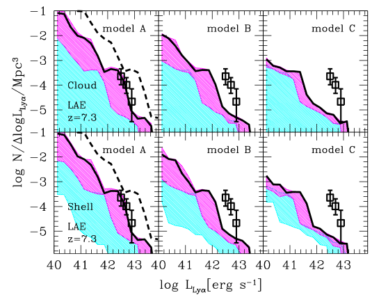
Figure 6: $\rm{Ly{\alpha}}$ luminosity functions (LFs) at $z=7.3$. Square symbols represent the observed LF of LAEs at $z=7.3$ by Konno et al. (2014). Upper and lower panels present modeled LFs using $\rm{Ly{\alpha}}$ line profiles of the cloud and shell models, respectively. Different panels from left to right show modeled LFs based on $\rm{Ly{\alpha}}$ line profiles to different Hi column densities. Magenta and cyan shades show the range of LFs considering $\rm{Ly{\alpha}}$ line profile with different outflow and inflow velocity with the range $0\sim\pm 300~{}\rm km~{}s^{-1}$. Black solid lines are best fitted ones to the observation. Black dash line in the left panel shows the LF before considering IGM transmission.

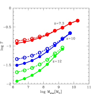
Figure 7: IGM transmission as a function of stellar mass of galaxies. Filled and open circles represent median values of the cloud and shell models, respectively. Different colors indicate different redshifts.

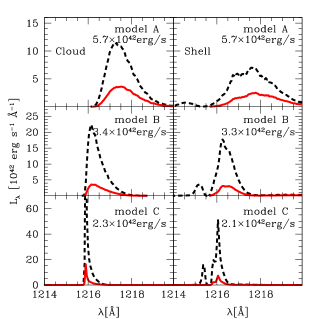
Figure 8: $\rm{Ly{\alpha}}$ line profiles. Red solid lines show emergent line profiles of a halo of $5.9\times 10^{11}~{}\rm{M_{\odot}}$ at z=7.3, which evolves to a halo of $1.0\times 10^{12}~{}\rm{M_{\odot}}$ at $z=6.0$. Intrinsic $\rm{Ly{\alpha}}$ luminosity of the halo is $1.3\times 10^{43}~{}{\rm erg~{}s^{-1}}$. Left and right panels represent the $\rm{Ly{\alpha}}$ line profiles of the cloud and shell models. Emergent luminosities after IGM transmission are shown in the panels. Black dash lines are the line profiles before considering IGM transmission.

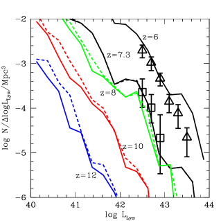
Figure 9: $\rm{Ly{\alpha}}$ luminosity functions at $z=6,7.3,8,10$ and $12$. Open triangles and squares show observed LAEs at $z=5.7$ (Ouchi et al. 2008) and $7.3$ (Konno et al. 2014). Solid and dash lines represent the LFs based on the cloud and shell models. Solid line at $z=6$ shows the LF without the IGM attenuation.

3.3 Relation between Ly$\alpha$ luminosity and stellar mass

Figure 10 shows the sizes of Hii bubbles and $\rm{Ly{\alpha}}$ luminosities considering the IGM transmission. $\rm{Ly{\alpha}}$ properties are calculated by using the $\rm{Ly{\alpha}}$ profile of model A of the cloud model. The shades represent the range of $25\%-75\%$ in the sample. We see that $R_{\rm HII}$ tightly correlate with stellar mass, as $R_{\rm HII}\propto M_{\rm{star}}^{1/3}$, while the relation with SFR shows a large dispersion.

SFR rapidly increase by major merger. However, $R_{\rm HII}$ is not so sensitive to the short-time fluctuation of SFR because of the longer time-scale for reaching the ionization equilibrium state. As a result, the relation between $R_{\rm HII}$ and SFR shows the large dispersion. High-redshift galaxies have been observed as so-called Lyman-break galaxies (LBGs: Bouwens et al. 2012), via the Lyman-break technique so far. Our results indicate LBGs at $z\gtrsim 7$ with similar UV brightness can have different $\rm{Ly{\alpha}}$ fluxes due to the scatter of IGM transmission. At $z=15$, our sample is limited by the stellar mass of galaxies $M_{\rm{star}}\sim 10^{9}~{}\rm{M_{\odot}}$. In our model, since the stellar mass is simply proportional to halo mass as $M_{\rm{star}}\sim 3.3\times 10^{-3}~{}M_{\rm h}$, this means that there is no progenitors with $M_{\rm h}\gtrsim 3\times 10^{11}~{}\rm{M_{\odot}}$ at $z=15$ in our halo sample, which is constructed to have the mass range from $10^{9}$ to $10^{13}~{}\rm{M_{\odot}}$ at $z=6$.

In contrast to the SFR-$R_{\rm HII}$ relation, both $\rm{Ly{\alpha}}$ luminosity and $R_{\rm HII}$ tightly correlate with $M_{\rm{star}}$. The $L_{\rm Ly\alpha}$-$M_{\rm{star}}$ relation does not change with redshift significantly, while the $R_{\rm HII}$-$M_{\rm{star}}$ becomes smaller as redshift increases. This is because Hubble constant (i.e., expanding velocity of IGM) becomes large at higher redshift. Therefore, although $R_{\rm HII}$ decreases as redshift increases due to higher IGM density, the IGM transmission does not decreases significantly. Thus, $\rm{Ly{\alpha}}$ luminosity does not depend sensitively on redshift. Note that, however, we have not taken the overlaps of Hii bubbles into account. When galaxies are clustered, giant Hii bubbles can form by the overlaps of individual Hii bubbles. This can cause scatters in the relations between $M_{\rm{star}}$ and $L_{\rm Ly\alpha}$ or $R_{\rm HII}$.

The detection sensitivity of recent observations of LAEs at $z\sim 7-8$ was corresponding to $\rm{Ly{\alpha}}$ luminosity of $\gtrsim 3\times 10^{42}~{}\rm{\rm erg~{}s^{-1}}$ (Ono et al. 2012; Shibuya et al. 2012; Finkelstein et al. 2013; Vanzella et al. 2011; Konno et al. 2014; Zitrin et al. 2015). In our model, median and minimum stellar masses producing $L_{\rm Ly\alpha}\sim 3\times 10^{42}~{}\rm erg~{}s^{-1}$ at $z=7.3$ are $6.5\times 10^{9}$ and $1.5\times 10^{8}~{}\rm{M_{\odot}}$, respectively. Therefore, by considering the relation $M_{\rm{star}}\sim 3.3\times 10^{-3}~{}M_{\rm h}$, we suggest that the observed LAEs at $z=7.3$ should be hosted in halos with $M_{\rm h}\geq 4.6\times 10^{10}~{}\rm{M_{\odot}}$, and the median halo mass is $1.9\times 10^{12}~{}\rm{M_{\odot}}$.

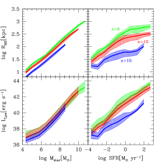
Figure 10: Upper panel: Sizes of Hii bubbles as a function of stellar mass and SFR. Green, red and blue lines represent median values to galaxies at $z=8,10$ and $15$, respectively. The shades show quartiles at each bin. Lower panel: $\rm{Ly{\alpha}}$ luminosity using the cloud model as a function of stellar mass and SFR.

3.4 Redshift evolution of number density of observable LAEs

So far the $\rm{Ly{\alpha}}$ line has been used as the most strong tool to confirm the redshift of distant galaxy candidates (e.g., Iye et al. 2006; Finkelstein et al. 2013; Zitrin et al. 2015). However, it is widely thought that LAEs at $z>9$ are difficult to be detected because of the IGM opacity. Here, we estimate the number density of LAEs ($n_{\rm LAE}$) with higher $\rm{Ly{\alpha}}$ flux than specific thresholds. Figure 11 shows the number density of LAEs with $F_{\rm\rm{Ly{\alpha}}}\geq 10^{-17},10^{-18}$ and $10^{-19}~{}\rm erg~{}s^{-1}~{}cm^{-2}$. The detection limits of current observations with a reasonable integration time are $\sim 10^{-17}~{}\rm erg~{}s^{-1}~{}cm^{-2}$ (e.g., Shibuya et al. 2012). As explained in Sec. 3.2, the number density of bright LAEs monotonically decreases with increasing redshift. Given the detection limits of $10^{-17}~{}\rm erg~{}s^{-1}~{}cm^{-2}$, wide field surveys of $~{}100^{3}~{}\rm Mpc^{3}$ are able to detect LAEs up to $z\sim 8.5$. This is consistent with recent observed LAEs at $z\lesssim 9$ (Finkelstein et al. 2013; Oesch et al. 2015; Zitrin et al. 2015). The LAEs with $F_{\rm\rm{Ly{\alpha}}}\geq 10^{-17}$ at $z\sim 10$ are quite rare, with $n_{\rm LAE}\sim 1-2~{}\rm Gpc^{-3}$.

Spectroscopies of next generation telescopes, e.g., JWST, are supposed to achieve the sensitivity of $\sim 10^{-18}~{}\rm erg~{}s^{-1}~{}cm^{-2}$ with a reasonable integration time. If galaxies at $z\sim 10$ have outflowing gas with $v\gtrsim 100~{}\rm km~{}s^{-1}$, the number density of LAEs with $F_{\rm Ly\alpha}\geq 10^{-18}~{}\rm erg~{}s^{-1}~{}cm^{-2}$ at $z\sim 10$ is $\sim$ a few $\times 10^{-6}~{}\rm Mpc^{-3}$. As shown in Figure 10, bright LAEs are hosted in massive halos. The median halo and stellar mass of LAEs with $F_{\rm Ly\alpha}\geq 10^{-18}~{}\rm erg~{}s^{-1}~{}cm^{-2}$ at $z=10$ are $1.1\times 10^{12}$ and $3.5\times 10^{9}~{}\rm{M_{\odot}}$, respectively. It was suggested that the observed LBG at $z=11.1$, GNz11, had the stellar mass of $\sim 10^{9}~{}\rm{M_{\odot}}$ (Oesch et al. 2016), which is corresponding to $F_{\rm Ly\alpha}\sim 0.2\times 10^{-18}~{}\rm erg~{}s^{-1}~{}cm^{-2}$ in our model. Hence, it will be challenging to detect $\rm{Ly{\alpha}}$ flux from GNz11 even by future spectroscopies with the line sensitivity of $F_{\rm Ly\alpha}\sim 10^{-18}~{}\rm erg~{}s^{-1}~{}cm^{-2}$.

Different line profile models predict different number densities of observable LAEs. The IGM transmission becomes more sensitive to the intrinsic $\rm{Ly{\alpha}}$ line profile models, since the typical size of Hii bubbles gets smaller with increasing redshift. As a result, the difference of $n_{\rm LAE}$ among model A, B and C becomes larger at higher redshift, and more than order unity at $z\sim 10$. Future observation would also allow us to discriminate intrinsic line profiles, which in turn provide information about Hi column density and outflow velocity, by comparing the observed number density of LAEs with the theoretical models. On the other hand, it is difficult to distinguish the cloud and shell models from the number density alone as shown in the figure.

Even next generation telescopes, e.g., GMT, E-ELT, TMT, will be difficult to have the sensitivity of $\sim 10^{-19}~{}\rm erg~{}s^{-1}~{}cm^{-2}$. However, if future telescopes somehow achieve such a high sensitivity, wide field surveys of $\sim 100^{3}~{}\rm Mpc^{3}$ would be able to reach LAEs at $z\sim 12$.

In this work, we consider isolated Hii bubbles associated with individual LAEs in the estimation of IGM transmission. However, at lower redshift, Hii bubbles can be overlapped each other (e.g., Iliev et al. 2012; Hasegawa & Semelin 2013; Ocvirk et al. 2016). The overlapped Hii bubbles can enhance the IGM transmission. This effect will be investigated in Hasegawa et al. (in preparation) by combining large-scale $N$-body with small scale radiative-hydrodynamics simulations.

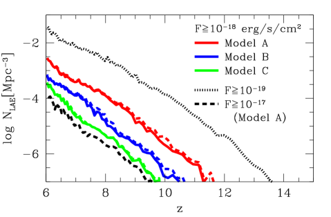
Figure 11: Number density of LAEs as a function of redshift. Red, blue and green lines show the number densities of LAEs with $F_{\rm{Ly{\alpha}}}\geq 10^{-18}~{}\rm erg\,cm^{-2}\,s^{-1}$ obtained assuming $\rm{Ly{\alpha}}$ line profiles of model A, B and C, respectively. Colored solid and dash lines represent the number density using the line profiles of the cloud and shell models. Black dash and dot lines are the number density of LAEs with $F_{\rm{Ly{\alpha}}}\geq 10^{-17}~{}\rm erg\,cm^{-2}\,s^{-1}$ and $F_{\rm{Ly{\alpha}}}\geq 10^{-19}~{}\rm erg\,cm^{-2}\,s^{-1}$ obtained assuming the $\rm{Ly{\alpha}}$ line profile of model A of the cloud model.

Table 1: Model parameters

Model	$N_{\rm HI}/{\rm cm^{2}}$	$V_{\rm out}/{\rm km\,s^{-1}}$ (cloud)	$V_{\rm out}/{\rm km\,s^{-1}}$ (shell)
A	$2\times 10^{20}$	180	130
B	$2\times 10^{19}$	190	60
C	$2\times 10^{18}$	110	40
	$f_{\rm esc,ion}=0.2$
	$f_{\rm esc,UV}=0.6$
	$f_{\rm esc,Ly\alpha}=0.6$

NOTES.—For each Hi column density, the outflow velocity is chosen to reproduce the observed luminosity function of LAE at $z=7.3$ (Konno et al. 2014). $V_{\rm out}$ (cloud) and $V_{\rm out}$ (shell) represent best-fitted outflow velocities in the expanding cloud and shell models. Escape fractions of ionizing, UV and $\rm{Ly{\alpha}}$ photons are same for all models.

4 Discussion

4.1 Impact of overlap of Hii bubbles on $\rm{Ly{\alpha}}$ radiation properties

So far, we consider only isolated Hii bubbles around LAEs. However, due to the clustering of galaxies, Hii bubbles overlap each other (e.g., McQuinn et al. 2007b; Zahn et al. 2011; Iliev et al. 2012). This leads to the expansion of the size of Hii bubbles, resulting in the increase of IGM transmission. Recently, Castellano et al. (2016) observed two LAEs in a galaxy overdensity region at $z\sim 7$ that might imply the clustering galaxies made a giant Hii bubble. Here, considering the overlap effect, we artificially expand sizes of all Hii bubbles associated with galaxies as follows:

$$R_{\rm HII}^{\prime}=f_{\rm boost}^{\rm HII}R_{\rm HII},$$ (12)

where $f_{\rm boost}^{\rm HII}$ is the boost factor to expand the original size of Hii bubbles. For example, the condition of $f_{\rm boost}^{\rm HII}=2$ roughly considers that $\sim 8$ galaxies with similar luminosities distribute in an overlapped Hii bubble, since the size of the Hii bubbles is proportional to the power of one-third of luminosities. In practice, $f_{\rm boost}^{\rm HII}$ can depend on original sizes of Hii bubbles. Small Hii bubbles associated with low-mass galaxies near massive ones can be merged into giant Hii bubbles, resulting in high $f_{\rm boost}^{\rm HII}$. On the other hand, the overlap between giant Hii bubbles is not frequent, leading to low $f_{\rm boost}^{\rm HII}$.

As the size of Hii bubbles increases by the overlap effect, even $\rm{Ly{\alpha}}$ photons with the line center frequency can penetrate IGM. This is likely to affect the outflow velocity to reproduce the observation. Figure 12 represents the best-fit outflow-velocities reproducing the observed LF at $z=7.3$ as a function of $f_{\rm boost}^{\rm HII}$. Due to the expansion of Hii bubbles, the modeled LFs shift to brighter side, i.e., right side along x-axis in Figure 6. Therefore, as $f_{\rm boost}^{\rm HII}$ increases, the best-fit outflow-velocities monotonically decrease. All models show that the velocities become smaller than $\sim 50~{}\rm km~{}s^{-1}$ at $f_{\rm boost}^{\rm HII}\gtrsim 3$. However, in the range of $f_{\rm boost}^{\rm HII}=1-4$, the velocities do not go below $0~{}\rm km~{}s^{-1}$, i.e., the LFs with $V=0~{}\rm km~{}s^{-1}$ do not exceed the observed LF. Therefore, if typical value of $f_{\rm boost}^{\rm HII}$ is smaller than 4, LAEs are likely to have outflowing gas.

The two-point correlation functions of LAEs derived from recent LAE surveys at $z=6.6$ showed the typical correlation length $r_{0}$ was $\sim 3~{}\rm Mpc$ in comoving scale and corresponding halo mass was $\sim 10^{11}~{}\rm{M_{\odot}}$ (Ouchi et al. 2010, 2017). The correlation length of LAEs does not change with redshift significantly (Ouchi et al. 2010). In our model, the Hii bubble size around halos of $\sim 10^{11}~{}\rm{M_{\odot}}$ is $\sim 260~{}\rm kpc$. The fact that the Hii bubble size is typically smaller than $r_{0}$ might indicate that $f_{\rm boost}^{\rm HII}$ does not largely exceed unity. The detailed overlap effect should be investigated by future cosmological simulations.

The velocities of model B and C of the cloud model does not change largely even if $f_{\rm boost}^{\rm HII}$ increases. As seen in Figure 5, the shell model with a large outflow velocity produces the strong peaks at the line center frequency. Therefore, even if $f_{\rm boost}^{\rm HII}$ is small, the velocities of the shell model do not increase largely.

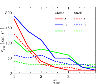
Figure 12: Outflow velocities matching the observed luminosity function as a function of the boost factor of Hii bubble size. The IGM transmission is calculated to Hii bubble extended artificially, $r^{\prime}_{\rm HII}=f_{\rm boost}^{\rm HII}\times r_{\rm HII}$. Solid and dash lines represent the expanding cloud and shell models, respectively. Different colors indicate different Hi column densities in the calculations of line profiles.

4.2 Condition for galactic outflow from LAEs

As shown in Section 3.2, high-redshift LAEs are likely to have galactic wind with $V_{\rm out}\gtrsim 100~{}\rm\rm km\;s^{-1}$. Here we roughly derive the condition for making gas outflow with $V_{\rm out}\gtrsim 100~{}\rm\rm km\;s^{-1}$ in a spherical gas cloud model. Supernova (SN) feedback can be responsible for causing strong outflow in high-redshift low-mass galaxies (e.g., Kimm & Cen 2014; Kimm et al. 2015). In the assumption that supernovae give feedback to all gas uniformly, we estimate the total kinetic energy of outflowing gas as

$$\begin{split}\frac{1}{2}M_{\rm gas}V_{\rm out}^{2}\sim f_{\rm conv}e_{\rm SN}N_{\rm SN}-\frac{GM_{\rm h}M_{\rm gas}}{R_{\rm vir}}.\end{split}$$ (13)

Here $M_{\rm gas}=(1-\epsilon)M_{\rm gas}^{0}$ is gas mass after star formation, $M_{\rm{star}}=\epsilon M_{\rm gas}^{0}$ is stellar mass, $M_{\rm gas}^{0}$ is initial gas mass, $\epsilon\equiv M_{\rm{star}}/M_{\rm gas}^{0}$ is a star formation efficiency with respect to the initial gas mass, $f_{\rm conv}$ is the conversion efficiency from total supernova energy to kinetic one of gas, $e_{\rm SN}\sim 2\times 10^{51}~{}\rm erg$ is the released energy for each supernova (e.g., Hamuy 2003), and $N_{\rm SN}$ is the number of supernova. For Salpeter-like IMF, $N_{\rm SN}\sim 1\times 10^{-2}\frac{M_{\rm{star}}}{\rm{M_{\odot}}}=1\times 10^{-2}\left(\frac{\epsilon}{1-\epsilon}\right)\frac{M_{\rm gas}}{\rm{M_{\odot}}}$. By using the star formation efficiency $\epsilon$, we simply estimate $V_{\rm out}$ as

$$\sqrt{V_{\rm out}^{2}+v_{\rm esc}^{2}}\sim 1.4\times 10^{3}~{}{\rm km~{}s^{-1}}~{}\left(\frac{\epsilon}{1-\epsilon}\right)^{\frac{1}{2}}f_{\rm conv}^{\frac{1}{2}},$$ (14)

where $v_{\rm esc}\equiv\sqrt{\frac{2GM_{\rm h}}{R_{\rm vir}}}$ is the escape velocity of a halo.

Next we obtain $f_{\rm conv}$ as a function of $\epsilon$. Recently Kim & Ostriker (2015) showed the final momentum produced by a single SN with the energy of $10^{51}~{}\rm erg$ as follows: $p=2.8\times 10^{5}~{}{\rm\rm km\;s^{-1}~{}\rm{M_{\odot}}}\left(\frac{n_{\rm H}}{1~{}\rm cm^{-3}}\right)^{-0.17}$ (see also, Cioffi et al. 1988; Thornton et al. 1998). In this work, we ignore the weak density dependence and assume $n_{\rm H}\sim 1~{}\rm cm^{-3}$. Since the final momentum is almost linearly proportional to the injected SN energy (Cioffi et al. 1988; Kimm & Cen 2014), we approximate the total momentum produced by multiple SNe as follows: $P=p\left(\frac{e_{\rm SN}N_{\rm SN}}{10^{51}~{}\rm erg}\right)$, where $e_{\rm SN}N_{\rm SN}$ is the total energy of supernovae. Therefore, using $E=\frac{P^{2}}{2M_{\rm gas}}$, we derive $f_{\rm conv}=\frac{E}{E_{\rm SN}}=16\left(\frac{\epsilon}{1-\epsilon}\right)$. Note that $f_{\rm conv}$ can not exceed unity according to the energy conservation. For that reason, we set $f_{\rm conv}=1$ at $\epsilon\geq 0.06$ because the above expression gives $f_{\rm conv}>1$. Thus, Equation 14 is written by using $\epsilon$ as follows:

$$\sqrt{V_{\rm out}^{2}+v_{\rm esc}^{2}}\sim\begin{cases}5.5\times 10^{3}~{}{\rm km~{}s^{-1}}~{}\left(\frac{\epsilon}{1-\epsilon}\right)\\ ~{}~{}~{}~{}~{}~{}~{}~{}~{}~{}~{}~{}~{}~{}~{}~{}~{}~{}~{}~{}~{}~{}~{}~{}~{}~{}~{}~{}~{}~{}~{}~{}~{}{\rm if}~{}~{}\epsilon<0.06\\ 1.4\times 10^{3}~{}{\rm km~{}s^{-1}}~{}\left(\frac{\epsilon}{1-\epsilon}\right)^{\frac{1}{2}}\\ ~{}~{}~{}~{}~{}~{}~{}~{}~{}~{}~{}~{}~{}~{}~{}~{}~{}~{}~{}~{}~{}~{}~{}~{}~{}~{}~{}~{}~{}~{}~{}~{}~{}{\rm if}~{}~{}\epsilon\geq 0.06.\end{cases}$$ (15)

We find that the condition of $\epsilon\sim 0.04$ is required to cause the galactic outflow with $V_{\rm out}=180~{}\rm\rm km\;s^{-1}$ from a halo with $M_{\rm h}=4.6\times 10^{10}~{}\rm{M_{\odot}}$ at $z=7.3$ which is minimum halo mass to produce the observable $\rm{Ly{\alpha}}$ luminosity $\sim 3\times 10^{42}~{}\rm erg~{}s^{-1}$. We can also convert the tuning parameter $\alpha$ in our star formation model to $\epsilon$, as $\epsilon\sim\alpha\Omega_{\rm M}/\Omega_{\rm b}\sim 0.02$. This is roughly similar to the value estimated above. As halo mass increases, higher $\epsilon$ is required to cause galactic outflow. Here we have estimated $\epsilon$ assuming all gas has same outflow velocity in the simple spherical cloud model. For example, in the case of disk galaxies, only a part of gas can be evacuated along the normal direction to galactic disk as shown in numerical simulations (e.g., Agertz et al. 2011). In this case, strong outflow can be caused even with smaller $\epsilon$ because piled gas mass can be lower.

4.3 Relation between Ly$\alpha$ luminosity and size of ionized bubble

LAEs can be responsible for ionizing sources of cosmic reionization (e.g., Yajima et al. 2009, 2011, 2014). Figure 13 shows $L_{\rm Ly\alpha}$ as a function of the size of associated Hii bubble $R_{\rm HII}$. The $\rm{Ly{\alpha}}$ luminosity steeply increases with $R_{\rm HII}$ due to higher IGM transmission for large Hii bubbles. The relation between $L_{\rm Ly\alpha}$ and $R_{\rm HII}$ does not significantly change with redshift. IGM gas density increases with redshift as $\rho\propto(1+z)^{3}$, resulting in lower IGM transmission at higher redshift. However, galaxies tend to have higher ionizing photon emissivity and intrinsic $\rm{Ly{\alpha}}$ luminosity for a fixed size of Hii bubbles at higher redshift. The combination of these effects leads to the weak redshift dependence in the $L_{\rm Ly\alpha}$-$R_{\rm HII}$ relation.

The yellow shaded region represents the viewing angle of $\geq 1$ arcmin and the flux of $\geq 10^{-18}~{}\rm erg~{}s^{-1}~{}cm^{-2}$ for $z\sim 10$. This region corresponds to the LAEs with associated Hii bubbles that are detectable both as LAEs and holes in 21-cm signal by future galaxy observations by JWST and 21-cm tomography by SKA-2, respectively. Future 21-cm observations will be able to probe giant Hii bubbles around bright LAEs with $F_{\rm Ly\alpha}\gtrsim 10^{-18}~{}\rm erg~{}s^{-1}~{}cm^{-2}$ at $z\sim 10$. Note that, the overlap of Hii bubbles is not considered in Figure 13. The effect of the overlap can shift our results to larger side of the Hii bubble.

The differential brightness temperature $\delta T_{\rm b}$ caused by galaxies shows inner positive and outer negative ring-like structure (e.g., Chen & Miralda-Escudé 2004; Yajima & Li 2014). The detailed structure depends on SED. If galaxies host X-ray sources like AGNs, the positive region is extended due to partial photo-ionization heating. Therefore, future 21-cm observations may also give us information about nature of X-ray and UV sources in bright LAEs.

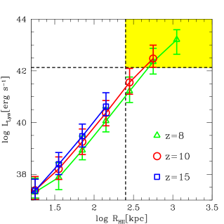
Figure 13: $\rm{Ly{\alpha}}$ luminosity as a function of size of Hii bubble. Triangle, circle and square symbols represent median values at $z=8,10$ and $15$, respectively. Error bars show quartiles. The $\rm{Ly{\alpha}}$ line profile of model A is used. Horizontal dash line shows $\rm{Ly{\alpha}}$ flux of $10^{-18}~{}\rm erg\,cm^{-2}\,s^{-1}$ for $z=10$. Vertical dash line represents the viewing angle of 1 arcmin for $z=10$.

4.4 Limitations in current models

Here we have investigated properties of LAEs and ionized bubbles at the era of reionization based on simple analytical models. Our current model is not able to consider following important aspects.

(1) redshift evolution of parameters: In this work, we have assumed the escape fraction of $\rm{Ly{\alpha}}$ photons and the shape of $\rm{Ly{\alpha}}$ line profile did not change with redshift. These quantities depend on physical properties of interstellar medium that can change with redshift (e.g., Mao et al. 2007; Yajima et al. 2014).

(2) overlap of ionized bubbles: As ionized bubbles grow, they overlap each other, leading to formation of giant Hii bubbles. This increases the IGM transmission of $\rm{Ly{\alpha}}$ photons with the frequency near the line center.

(3) $\rm{Ly{\alpha}}$ surface brightness: Multiple scattering processes of $\rm{Ly{\alpha}}$ photons in galaxies can make extended $\rm{Ly{\alpha}}$ surface brightness distribution. Recent observations indicated star-forming galaxies had extended $\rm{Ly{\alpha}}$ haloes (e.g., Steidel et al. 2011; Momose et al. 2014, 2016). Therefore, some fraction of $\rm{Ly{\alpha}}$ flux could be lost in the observations of LAEs. Understanding the $\rm{Ly{\alpha}}$ surface brightness distribution and the flux loss are quite important in liking between theoretical models and observations. However, the fraction of lost $\rm{Ly{\alpha}}$ flux sensitively depends on the sensitivities of the observations, and it is uncertain now. In this work, we have assumed that all $\rm{Ly{\alpha}}$ photons escaped from galaxies can be observed, if they are not scatted by IGM. This assumption can be reasonable when sizes of galaxies are not much larger than angular resolutions of $\rm{Ly{\alpha}}$ observations. Recently Mas-Ribas et al. (2017) showed JWST will be able to reach the sensitivity $\sim 10^{-20}~{}\rm erg~{}cm^{-2}~{}s^{-1}~{}arcsec^{-2}$ for extended emission sources. Here we roughly estimate the surface brightness as $S_{\rm{Ly{\alpha}}}\sim\frac{F_{\rm{Ly{\alpha}}}}{\pi r_{\rm edge}^{2}}$. For detections of bright LAEs of $F\sim 10^{-18}~{}\rm erg~{}cm^{-2}~{}s^{-1}$, the source size should be smaller than $\sim 6~{}\rm arcsec$, corresponding to $r_{\rm edge}\sim 30~{}\rm kpc$ at $z\sim 7$. This is comparable with the virial radius of halos with masses of $10^{11}-10^{12}~{}\rm{M_{\odot}}$. Therefore the flux loss due to the faint surface brightness is unlikely to be significant. In addition, Momose et al. (2014) suggested that typical scale lengths of $\rm{Ly{\alpha}}$ halos of observed LAEs at $z\sim 2-6$ were $\sim 5-10~{}\rm kpc$ and do not change with redshift significantly. Note that, however, the surface brightness sensitively depends on complicated distributions of gas and velocity fields (e.g., Yajima et al. 2015). In reality, the surface brightness distribution should be considered in the estimation of the flux loss for extended sources, which is beyond the scope in this paper. We will study the detectability of distant LAEs with the calculation of surface brightness by combining cosmological hydrodynamics simulations and $\rm{Ly{\alpha}}$ radiative transfer calculations in future work.

5 Summary

We present models of $\rm{Ly{\alpha}}$ emitting galaxies (LAEs) with IGM transmission considered at the era of reionization. Based on halo merger trees and a simple star formation model, we estimate cosmic star formation and cosmic reionization history. Our model uses 5000 realizations of halo merger trees with the halo mass range from $M_{\rm h}=10^{9}$ to $10^{13}~{}\rm{M_{\odot}}$ at $z=6$. As a result, our model reproduces the observed cosmic star formation densities, stellar mass densities, luminosity functions of Lyman-break galaxies with a tuning parameter, $\alpha(\equiv SFR/\frac{dM_{\rm h}}{dt})=3.3\times 10^{-3}$. Our modeled star formation history, with an escape fraction of ionizing photons $f_{\rm esc,ion}=0.2$, also provides a cosmic reionization history consistent with the Thomson scattering optical depth indicated by Plank (2016).

Based on the above parameters, we model LAEs and Hii bubbles using individual halo merger trees. Our models show the distribution function of the size of Hii bubble, and indicate giant Hii bubbles associated with bright LAEs at $z\lesssim 12$ can be probed by future 21-cm observation using SKA. We find that $\rm{Ly{\alpha}}$ flux is tightly related with stellar/halo mass, while there is a large dispersion in the relation between $\rm{Ly{\alpha}}$ flux and SFR. By comparing our models with the observed luminosity function of LAEs at $z=7.3$ by Konno et al. (2014), we indicate that LAEs are likely to have the Hi column density of $N_{\rm HI}\gtrsim 10^{20}~{}\rm cm^{-2}$ and the outflowing gas with $V_{\rm out}\gtrsim 100~{}\rm\rm km\;s^{-1}$. Using these parameters, we predict that future wide deep survey can detect LAEs at $z\sim 10$ with $n_{\rm LAE}\sim{\rm a~{}few~{}}\times 10^{-6}~{}\rm Mpc^{-3}$ and $\sim 1\times 10^{-4}~{}\rm Mpc^{-3}$ for the flux sensitivity of $10^{-18}~{}\rm erg\,cm^{-2}\,s^{-1}$ and $10^{-19}~{}\rm erg\,cm^{-2}\,s^{-1}$, respectively. Our models predict next generation telescopes, JWST, E-ELT or TMT would be able to observe galaxies at $z\sim 10$ via the detections of $\rm{Ly{\alpha}}$ lines.

By combining future galaxy observations and 21-cm tomography with SKA-2, we will be able to detect both LAEs with $L_{\rm Ly\alpha}\gtrsim 10^{42}~{}{\rm erg~{}s^{-1}}$ and their associated giant Hii bubbles with $R_{\rm HII}\gtrsim 250~{}\rm kpc$. We suggest that a clear spatial anti-correlation between galaxies and 21-cm emission will be detected by focusing on such bright LAEs. Here we consider individual Hii bubbles associated LAEs alone. However, when galaxies distribute in clustering regions, the Hii bubbles overlap each other, resulting in the formation of giant Hii bubbles. Therefore, this can cause a large dispersion in the relation between the bubble size and $\rm{Ly{\alpha}}$ luminosity.

In this work, we assume that the Hi column density and outflow velocity do not change significantly with redshift. On the other hand, Konno et al. (2016) suggested that Hi column density should decrease as the redshift increases over the redshift range $z\sim 2-6$ in order to reproduce the redshift evolution of observed $\rm{Ly{\alpha}}$ escape fraction. They suggested that LAEs at $z\sim 6$ should have the Hi column density of $\sim 10^{18}~{}\rm cm^{-2}$ to obtain the high $\rm{Ly{\alpha}}$ escape fraction. However, the relation between the Hi column density and the escape fraction can be changed due to physical properties of ISM. Recently Gronke & Dijkstra (2016) have introduced some detailed properties of ISM into their expanding shell models, e.g., clumpiness. The porous ISM can reproduce high escape fraction even for high Hi column density. This can alleviate the discrepancy between our models and Konno et al. (2016). Note that, in our model, the high Hi column density has been favored to obtain reasonable IGM transmissions for reproducing the observed luminosity function. However, when the overlaps of Hii bubbles are considered, even somewhat lower Hi column density can be allowed. Lower Hi column density leads to the smaller shift of the peak frequency of $\rm{Ly{\alpha}}$ line profile, resulting in lower IGM transmission. Therefore, the number density of observable LAEs at $z\gg 7$ becomes smaller than the above estimation, if the Hi column density decreases.

In addition, the flux loss due to limited sensitivities in observations has not been taken into account in our current models. Even the high-sensitivity of JWST can lose some fraction of total flux if high-$z$ LAEs are very extended due to $\rm{Ly{\alpha}}$ scattering in ISM.

Thus our estimation of detectability for LAEs at $z\gtrsim 10$ might be somewhat optimistic. We will investigate the $\rm{Ly{\alpha}}$ line profiles and the surface brightness distribution by combining cosmological hydrodynamics simulations and $\rm{Ly{\alpha}}$ radiative transfer calculations in our future work.

References

- Agertz et al. (2011) Agertz O., Teyssier R., Moore B., 2011, MNRAS, 410, 1391
- Barkana & Loeb (2001) Barkana R., Loeb A., 2001, Phys. Rep., 349, 125
- Behroozi & Silk (2015) Behroozi P. S., Silk J., 2015, ApJ, 799, 32
- Behroozi et al. (2013) Behroozi P. S., Wechsler R. H., Conroy C., 2013, ApJ, 770, 57
- Bolton & Haehnelt (2013) Bolton J. S., Haehnelt M. G., 2013, MNRAS, 429, 1695
- Bond et al. (2011) Bond N., Gawiser E., Guaita L., Padilla N., Gronwall C., Ciardullo R., Lai K., 2011, ArXiv e-prints
- Bouwens et al. (2015) Bouwens R. J., Illingworth G. D., Oesch P. A., Trenti M., Labbé I., Bradley L., Carollo M., van Dokkum P. G., Gonzalez V., Holwerda B., Franx M., Spitler L., Smit R., Magee D., 2015, ApJ, 803, 34
- Bouwens et al. (2012) Bouwens R. J., Illingworth G. D., Oesch P. A., Trenti M., Labbé I., Franx M., Stiavelli M., Carollo C. M., van Dokkum P., Magee D., 2012, ApJ, 752, L5
- Bullock et al. (2001) Bullock J. S., Kolatt T. S., Sigad Y., Somerville R. S., Kravtsov A. V., Klypin A. A., Primack J. R., Dekel A., 2001, MNRAS, 321, 559
- Cai et al. (2014) Cai Z.-Y., Lapi A., Bressan A., De Zotti G., Negrello M., Danese L., 2014, ApJ, 785, 65
- Castellano et al. (2016) Castellano M., Dayal P., Pentericci L., Fontana A., Hutter A., Brammer G., Merlin E., Grazian A., Pilo S., Amorin R., Cristiani S., Dickinson M., Ferrara A., Gallerani S., Giallongo E., Giavalisco M., Guaita L., Koekemoer A., Maiolino R., Paris D., Santini P., Vallini L., Vanzella E., Wagg J., 2016, ApJ, 818, L3
- Cen (2003) Cen R., 2003, ApJ, 591, 12
- Cen & Haiman (2000) Cen R., Haiman Z., 2000, ApJ, 542, L75
- Chen & Miralda-Escudé (2004) Chen X., Miralda-Escudé J., 2004, ApJ, 602, 1
- Choudhury et al. (2015) Choudhury T. R., Puchwein E., Haehnelt M. G., Bolton J. S., 2015, MNRAS, 452, 261
- Ciardi et al. (2012) Ciardi B., Bolton J. S., Maselli A., Graziani L., 2012, MNRAS, 423, 558
- Ciardullo et al. (2012) Ciardullo R., Gronwall C., Wolf C., McCathran E., Bond N. A., Gawiser E., Guaita L., Feldmeier J. J., Treister E., Padilla N., Francke H., Matković A., Altmann M., Herrera D., 2012, ApJ, 744, 110
- Cioffi et al. (1988) Cioffi D. F., McKee C. F., Bertschinger E., 1988, ApJ, 334, 252
- Dewdney et al. (2009) Dewdney P. E., Hall P. J., Schilizzi R. T., Lazio T. J. L. W., 2009, IEEE Proceedings, 97, 1482
- Dijkstra (2014) Dijkstra M., 2014, Publications of the Astronomical Society of Australia, 31, e040
- Dijkstra et al. (2006) Dijkstra M., Haiman Z., Spaans M., 2006, ApJ, 649, 14
- Dijkstra & Kramer (2012) Dijkstra M., Kramer R., 2012, MNRAS, 424, 1672
- Dijkstra et al. (2011) Dijkstra M., Mesinger A., Wyithe J. S. B., 2011, MNRAS, 548
- Fan et al. (2006) Fan X., Carilli C. L., Keating B., 2006, ARA&A, 44, 415
- Finkelstein et al. (2013) Finkelstein S. L., Papovich C., Dickinson M., Song M., Tilvi V., Koekemoer A. M., Finkelstein K. D., Mobasher B., Ferguson H. C., Giavalisco M., Reddy N., Ashby M. L. N., Dekel A., Fazio G. G., Fontana A., Grogin N. A., Huang J.-S., Kocevski D., Rafelski M., Weiner B. J., Willner S. P., 2013, Nature, 502, 524
- Furlanetto et al. (2004) Furlanetto S. R., Hernquist L., Zaldarriaga M., 2004, MNRAS, 354, 695
- Gawiser et al. (2007) Gawiser E., Francke H., Lai K., Schawinski K., Gronwall C., Ciardullo R., Quadri R., Orsi A., Barrientos L. F., Blanc G. A., Fazio G., Feldmeier J. J., Huang J.-s., Infante L., Lira P., Padilla N., Taylor E. N., Treister E., Urry C. M., van Dokkum P. G., Virani S. N., 2007, ApJ, 671, 278
- Gronke & Dijkstra (2016) Gronke M., Dijkstra M., 2016, ApJ, 826, 14
- Gronwall et al. (2007) Gronwall C., Ciardullo R., Hickey T., Gawiser E., Feldmeier J. J., van Dokkum P. G., Urry C. M., Herrera D., Lehmer B. D., Infante L., Orsi A., Marchesini D., Blanc G. A., Francke H., Lira P., Treister E., 2007, ApJ, 667, 79
- Hamuy (2003) Hamuy M., 2003, ApJ, 582, 905
- Harker et al. (2010) Harker G., Zaroubi S., Bernardi G., Brentjens M. A., de Bruyn A. G., Ciardi B., Jelić V., Koopmans L. V. E., Labropoulos P., Mellema G., Offringa A., Pandey V. N., Pawlik A. H., Schaye J., Thomas R. M., Yatawatta S., 2010, MNRAS, 405, 2492
- Hasegawa & Semelin (2013) Hasegawa K., Semelin B., 2013, MNRAS, 428, 154
- Henry et al. (2015) Henry A., Scarlata C., Martin C. L., Erb D., 2015, ApJ, 809, 19
- Hopkins et al. (2014) Hopkins P. F., Kereš D., Oñorbe J., Faucher-Giguère C.-A., Quataert E., Murray N., Bullock J. S., 2014, MNRAS, 445, 581
- Hu & McMahon (1996) Hu E. M., McMahon R. G., 1996, Nature, 382, 231
- Iliev et al. (2006) Iliev I. T., Mellema G., Pen U.-L., Merz H., Shapiro P. R., Alvarez M. A., 2006, MNRAS, 369, 1625
- Iliev et al. (2012) Iliev I. T., Mellema G., Shapiro P. R., Pen U.-L., Mao Y., Koda J., Ahn K., 2012, MNRAS, 423, 2222
- Inoue et al. (2013) Inoue Y., Inoue S., Kobayashi M. A. R., Makiya R., Niino Y., Totani T., 2013, ApJ, 768, 197
- Iye et al. (2006) Iye M., Ota K., Kashikawa N., Furusawa H., Hashimoto T., Hattori T., Matsuda Y., Morokuma T., Ouchi M., Shimasaku K., 2006, Nature, 443, 186
- Jensen et al. (2013) Jensen H., Laursen P., Mellema G., Iliev I. T., Sommer-Larsen J., Shapiro P. R., 2013, MNRAS, 428, 1366
- Jeon et al. (2014) Jeon M., Pawlik A. H., Bromm V., Milosavljević M., 2014, MNRAS, 440, 3778
- Kashikawa et al. (2006) Kashikawa N., Shimasaku K., Malkan M. A., Doi M., Matsuda Y., Ouchi M., Taniguchi Y., Ly C., Nagao T., Iye M., Motohara K., Murayama T., Murozono K., Nariai K., Ohta K., Okamura S., Sasaki T., Shioya Y., Umemura M., 2006, ApJ, 648, 7
- Khaire et al. (2016) Khaire V., Srianand R., Choudhury T. R., Gaikwad P., 2016, MNRAS, 457, 4051
- Khochfar & Burkert (2001) Khochfar S., Burkert A., 2001, ApJ, 561, 517
- Khochfar & Burkert (2006) —, 2006, A&A, 445, 403
- Kim & Ostriker (2015) Kim C.-G., Ostriker E. C., 2015, ApJ, 802, 99
- Kimm & Cen (2014) Kimm T., Cen R., 2014, ApJ, 788, 121
- Kimm et al. (2015) Kimm T., Cen R., Rosdahl J., Yi S., 2015, ArXiv e-prints
- Komatsu et al. (2011) Komatsu E., Smith K. M., Dunkley J., Bennett C. L., Gold B., Hinshaw G., Jarosik N., Larson D., Nolta M. R., Page L., Spergel D. N., Halpern M., Hill R. S., Kogut A., Limon M., Meyer S. S., Odegard N., Tucker G. S., Weiland J. L., Wollack E., Wright E. L., 2011, ApJS, 192, 18
- Konno et al. (2016) Konno A., Ouchi M., Nakajima K., Duval F., Kusakabe H., Ono Y., Shimasaku K., 2016, ApJ, 823, 20
- Konno et al. (2014) Konno A., Ouchi M., Ono Y., Shimasaku K., Shibuya T., Furusawa H., Nakajima K., Naito Y., Momose R., Yuma S., Iye M., 2014, ApJ, 797, 16
- Kravtsov et al. (2014) Kravtsov A., Vikhlinin A., Meshscheryakov A., 2014, ArXiv e-prints
- Laursen et al. (2009) Laursen P., Razoumov A. O., Sommer-Larsen J., 2009, ApJ, 696, 853
- Leitherer et al. (1999) Leitherer C., Schaerer D., Goldader J. D., Delgado R. M. G., Robert C., Kune D. F., de Mello D. F., Devost D., Heckman T. M., 1999, ApJS, 123, 3
- Lidz et al. (2009) Lidz A., Zahn O., Furlanetto S. R., McQuinn M., Hernquist L., Zaldarriaga M., 2009, ApJ, 690, 252
- Lonsdale et al. (2009) Lonsdale C. J., Cappallo R. J., Morales M. F., Briggs F. H., Benkevitch L., Bowman J. D., Bunton J. D., Burns S., Corey B. E., Desouza L., Doeleman S. S., Derome M., Deshpande A., Gopala M. R., Greenhill L. J., Herne D. E., Hewitt J. N., Kamini P. A., Kasper J. C., Kincaid B. B., Kocz J., Kowald E., Kratzenberg E., Kumar D., Lynch M. J., Madhavi S., Matejek M., Mitchell D. A., Morgan E., Oberoi D., Ord S., Pathikulangara J., Prabu T., Rogers A., Roshi A., Salah J. E., Sault R. J., Shankar N. U., Srivani K. S., Stevens J., Tingay S., Vaccarella A., Waterson M., Wayth R. B., Webster R. L., Whitney A. R., Williams A., Williams C., 2009, IEEE Proceedings, 97, 1497
- Madau & Haardt (2015) Madau P., Haardt F., 2015, ApJ, 813, L8
- Madau et al. (1999) Madau P., Haardt F., Rees M. J., 1999, ApJ, 514, 648
- Mao et al. (2007) Mao J., Lapi A., Granato G. L., de Zotti G., Danese L., 2007, ApJ, 667, 655
- Mas-Ribas et al. (2017) Mas-Ribas L., Hennawi J. F., Dijkstra M., Davies F. B., Stern J., Rix H.-W., 2017, ApJ, 846, 11
- McQuinn et al. (2007a) McQuinn M., Hernquist L., Zaldarriaga M., Dutta S., 2007a, MNRAS, 381, 75
- McQuinn et al. (2007b) McQuinn M., Lidz A., Zahn O., Dutta S., Hernquist L., Zaldarriaga M., 2007b, MNRAS, 377, 1043
- Mellema et al. (2006) Mellema G., Iliev I. T., Pen U.-L., Shapiro P. R., 2006, MNRAS, 372, 679
- Mesinger (2010) Mesinger A., 2010, MNRAS, 407, 1328
- Mesinger et al. (2015) Mesinger A., Aykutalp A., Vanzella E., Pentericci L., Ferrara A., Dijkstra M., 2015, MNRAS, 446, 566
- Mesinger & Furlanetto (2008) Mesinger A., Furlanetto S. R., 2008, MNRAS, 386, 1990
- Mo et al. (1998) Mo H. J., Mao S., White S. D. M., 1998, MNRAS, 295, 319
- Momose et al. (2014) Momose R., Ouchi M., Nakajima K., Ono Y., Shibuya T., Shimasaku K., Yuma S., Mori M., Umemura M., 2014, MNRAS, 442, 110
- Momose et al. (2016) —, 2016, MNRAS, 457, 2318
- Mori & Umemura (2006) Mori M., Umemura M., 2006, Nature, 440, 644
- Moster et al. (2013) Moster B. P., Naab T., White S. D. M., 2013, MNRAS, 428, 3121
- Ocvirk et al. (2016) Ocvirk P., Gillet N., Shapiro P. R., Aubert D., Iliev I. T., Teyssier R., Yepes G., Choi J.-H., Sullivan D., Knebe A., Gottlöber S., D’Aloisio A., Park H., Hoffman Y., Stranex T., 2016, MNRAS, 463, 1462
- Oesch et al. (2016) Oesch P. A., Brammer G., van Dokkum P. G., Illingworth G. D., Bouwens R. J., Labbé I., Franx M., Momcheva I., Ashby M. L. N., Fazio G. G., Gonzalez V., Holden B., Magee D., Skelton R. E., Smit R., Spitler L. R., Trenti M., Willner S. P., 2016, ApJ, 819, 129
- Oesch et al. (2015) Oesch P. A., van Dokkum P. G., Illingworth G. D., Bouwens R. J., Momcheva I., Holden B., Roberts-Borsani G. W., Smit R., Franx M., Labbé I., González V., Magee D., 2015, ApJ, 804, L30
- Okamoto et al. (2008) Okamoto T., Gao L., Theuns T., 2008, MNRAS, 390, 920
- Ono et al. (2012) Ono Y., Ouchi M., Mobasher B., Dickinson M., Penner K., Shimasaku K., Weiner B. J., Kartaltepe J. S., Nakajima K., Nayyeri H., Stern D., Kashikawa N., Spinrad H., 2012, ApJ, 744, 83
- Ouchi et al. (2017) Ouchi M., Harikane Y., Shibuya T., Shimasaku K., Taniguchi Y., Konno A., Kobayashi M., Kajisawa M., Nagao T., Ono Y., Inoue A. K., Umemura M., Mori M., Hasegawa K., Higuchi R., Komiyama Y., Matsuda Y., Nakajima K., Saito T., Wang S.-Y., 2017, ArXiv e-prints
- Ouchi et al. (2008) Ouchi M., Shimasaku K., Akiyama M., Simpson C., Saito T., Ueda Y., Furusawa H., Sekiguchi K., Yamada T., Kodama T., Kashikawa N., Okamura S., Iye M., Takata T., Yoshida M., Yoshida M., 2008, ApJS, 176, 301
- Ouchi et al. (2010) Ouchi M., Shimasaku K., Furusawa H., Saito T., Yoshida M., Akiyama M., Ono Y., Yamada T., Ota K., Kashikawa N., Iye M., Kodama T., Okamura S., Simpson C., Yoshida M., 2010, ApJ, 723, 869
- Paardekooper et al. (2013) Paardekooper J.-P., Khochfar S., Dalla Vecchia C., 2013, MNRAS, 429, L94
- Pawlik et al. (2009) Pawlik A. H., Schaye J., van Scherpenzeel E., 2009, MNRAS, 394, 1812
- Pentericci et al. (2016) Pentericci L., Carniani S., Castellano M., Fontana A., Maiolino R., Guaita L., Vanzella E., Grazian A., Santini P., Yan H., Cristiani S., Conselice C., Giavalisco M., Hathi N., Koekemoer A., 2016, ApJ, 829, L11
- Planck Collaboration et al. (2014) Planck Collaboration, Ade P. A. R., Aghanim N., Armitage-Caplan C., Arnaud M., Ashdown M., Atrio-Barandela F., Aumont J., Baccigalupi C., Banday A. J., et al., 2014, A&A, 571, A16
- Planck Collaboration et al. (2016) Planck Collaboration, Ade P. A. R., Aghanim N., Arnaud M., Ashdown M., Aumont J., Baccigalupi C., Banday A. J., Barreiro R. B., Bartlett J. G., et al., 2016, A&A, 594, A13
- Razoumov & Sommer-Larsen (2010) Razoumov A. O., Sommer-Larsen J., 2010, ApJ, 710, 1239
- Richards et al. (2006) Richards G. T., Strauss M. A., Fan X., Hall P. B., Jester S., Schneider D. P., Vanden Berk D. E., Stoughton C., Anderson S. F., Brunner R. J., Gray J., Gunn J. E., Ivezić Ž., Kirkland M. K., Knapp G. R., Loveday J., Meiksin A., Pope A., Szalay A. S., Thakar A. R., Yanny B., York D. G., Barentine J. C., Brewington H. J., Brinkmann J., Fukugita M., Harvanek M., Kent S. M., Kleinman S. J., Krzesiński J., Long D. C., Lupton R. H., Nash T., Neilsen Jr. E. H., Nitta A., Schlegel D. J., Snedden S. A., 2006, AJ, 131, 2766
- Robertson et al. (2015) Robertson B. E., Ellis R. S., Furlanetto S. R., Dunlop J. S., 2015, ApJ, 802, L19
- Robertson et al. (2013) Robertson B. E., Furlanetto S. R., Schneider E., Charlot S., Ellis R. S., Stark D. P., McLure R. J., Dunlop J. S., Koekemoer A., Schenker M. A., Ouchi M., Ono Y., Curtis-Lake E., Rogers A. B., Bowler R. A. A., Cirasuolo M., 2013, ApJ, 768, 71
- Sadoun et al. (2017) Sadoun R., Zheng Z., Miralda-Escudé J., 2017, ApJ, 839, 44
- Sheth & Tormen (2002) Sheth R. K., Tormen G., 2002, MNRAS, 329, 61
- Shibuya et al. (2012) Shibuya T., Kashikawa N., Ota K., Iye M., Ouchi M., Furusawa H., Shimasaku K., Hattori T., 2012, ApJ, 752, 114
- Shibuya et al. (2014) Shibuya T., Ouchi M., Nakajima K., Hashimoto T., Ono Y., Rauch M., Gauthier J.-R., Shimasaku K., Goto R., Mori M., Umemura. M., 2014, ApJ, 788, 74
- Somerville & Kolatt (1999) Somerville R. S., Kolatt T. S., 1999, MNRAS, 305, 1
- Song et al. (2016a) Song M., Finkelstein S. L., Ashby M. L. N., Grazian A., Lu Y., Papovich C., Salmon B., Somerville R. S., Dickinson M., Duncan K., Faber S. M., Fazio G. G., Ferguson H. C., Fontana A., Guo Y., Hathi N., Lee S.-K., Merlin E., Willner S. P., 2016a, ApJ, 825, 5
- Song et al. (2016b) Song M., Finkelstein S. L., Livermore R. C., Capak P. L., Dickinson M., Fontana A., 2016b, ApJ, 826, 113
- Spitzer (1978) Spitzer L., 1978, Physical processes in the interstellar medium, Spitzer, L., ed.
- Steidel et al. (2000) Steidel C. C., Adelberger K. L., Shapley A. E., Pettini M., Dickinson M., Giavalisco M., 2000, ApJ, 532, 170
- Steidel et al. (2011) Steidel C. C., Bogosavljević M., Shapley A. E., Kollmeier J. A., Reddy N. A., Erb D. K., Pettini M., 2011, ArXiv e-prints
- Tasitsiomi (2006) Tasitsiomi A., 2006, ApJ, 648, 762
- Thornton et al. (1998) Thornton K., Gaudlitz M., Janka H.-T., Steinmetz M., 1998, ApJ, 500, 95
- Tilvi et al. (2011) Tilvi V., Scannapieco E., Malhotra S., Rhoads J. E., 2011, ArXiv e-prints
- Trac & Cen (2007) Trac H., Cen R., 2007, ApJ, 671, 1
- Vanzella et al. (2011) Vanzella E., Pentericci L., Fontana A., Grazian A., Castellano M., Boutsia K., Cristiani S., Dickinson M., Gallozzi S., Giallongo E., Giavalisco M., Maiolino R., Moorwood A., Paris D., Santini P., 2011, ApJ, 730, L35
- Verhamme et al. (2015) Verhamme A., Orlitová I., Schaerer D., Hayes M., 2015, A&A, 578, A7
- Verhamme et al. (2008) Verhamme A., Schaerer D., Atek H., Tapken C., 2008, A&A, 491, 89
- Verhamme et al. (2006) Verhamme A., Schaerer D., Maselli A., 2006, A&A, 460, 397
- Wise et al. (2014) Wise J. H., Demchenko V. G., Halicek M. T., Norman M. L., Turk M. J., Abel T., Smith B. D., 2014, MNRAS, 442, 2560
- Wolfe et al. (2005) Wolfe A. M., Gawiser E., Prochaska J. X., 2005, ARA&A, 43, 861
- Wyithe et al. (2010) Wyithe J. S. B., Hopkins A. M., Kistler M. D., Yüksel H., Beacom J. F., 2010, MNRAS, 401, 2561
- Yajima et al. (2011) Yajima H., Choi J.-H., Nagamine K., 2011, MNRAS, 412, 411
- Yajima et al. (2012a) —, 2012a, MNRAS, 427, 2889
- Yajima & Khochfar (2015) Yajima H., Khochfar S., 2015, MNRAS, 448, 654
- Yajima & Li (2014) Yajima H., Li Y., 2014, MNRAS, 445, 3674
- Yajima et al. (2012b) Yajima H., Li Y., Zhu Q., Abel T., 2012b, MNRAS, 424, 884
- Yajima et al. (2014) Yajima H., Li Y., Zhu Q., Abel T., Gronwall C., Ciardullo R., 2014, MNRAS, 440, 776
- Yajima et al. (2015) Yajima H., Li Y., Zhu Q., Abel T., 2015, ApJ, 801, 52
- Yajima et al. (2017) Yajima H., Nagamine K., Zhu Q., Khochfar S., Dalla Vecchia C., 2017, ApJ, 846, 30
- Yajima et al. (2009) Yajima H., Umemura M., Mori M., Nakamoto T., 2009, MNRAS, 398, 715
- Yamada et al. (2012) Yamada T., Nakamura Y., Matsuda Y., Hayashino T., Yamauchi R., Morimoto N., Kousai K., Umemura M., 2012, AJ, 143, 79
- Yoshiura et al. (2016) Yoshiura S., Hasegawa K., Ichiki K., Tashiro H., Shimabukuro H., Takahashi K., 2016, ArXiv e-prints
- Zahn et al. (2011) Zahn O., Mesinger A., McQuinn M., Trac H., Cen R., Hernquist L. E., 2011, MNRAS, 414, 727
- Zitrin et al. (2015) Zitrin A., Labbé I., Belli S., Bouwens R., Ellis R. S., Roberts-Borsani G., Stark D. P., Oesch P. A., Smit R., 2015, ApJ, 810, L12