Corral Framework: Trustworthy and Fully Functional Data Intensive Parallel Astronomical Pipelines

Abstract

Data processing pipelines represent an important slice of the astronomical software library that include chains of processes that transform raw data into valuable information via data reduction and analysis. In this work we present Corral, a Python framework for astronomical pipeline generation. Corral features a Model-View-Controller design pattern on top of an SQL Relational Database capable of handling: custom data models; processing stages; and communication alerts, and also provides automatic quality and structural metrics based on unit testing. The Model-View-Controller provides concept separation between the user logic and the data models, delivering at the same time multi-processing and distributed computing capabilities. Corral represents an improvement over commonly found data processing pipelines in Astronomy since the design pattern eases the programmer from dealing with processing flow and parallelization issues, allowing them to focus on the specific algorithms needed for the successive data transformations and at the same time provides a broad measure of quality over the created pipeline. Corral and working examples of pipelines that use it are available to the community at https://github.com/toros-astro.

1 Introduction

The development of modern ground–based and space–born telescopes, covering all observable windows in the electromagnetic spectrum, and an ever increasing variability interest via time–domain astronomy have raised the necessity for large databases of astronomical observations. The amount of data to be processed has been steadily increasing, imposing higher demands over: quality; storage needs and analysis tools. This phenomenon is a manifestation of the deep transformation that Astronomy is going through, along with the development of new technologies in the Big Data era. In this context, new automatic data analysis techniques have emerged as the preferred solution to the so-called “data tsunami” (Cavuoti, 2013).

The development of an information processing pipeline is a natural consequence of science projects involving the acquisition of data and its posterior analysis. Some examples of these data intensive projects include The Dark Energy Survey Data Management System (Mohr et al., 2008), designed to exploit a camera with 74 CCDs at the Blanco telescope to study the nature of cosmic acceleration; the Infrared Processing and Analysis Center (Masci et al., 2016), a near real-time transient-source discovery engine for the intermediate Palomar Transient Factory (iPTF Kulkarni, 2013); and the Pan-STARRS PS1 Image Processing Pipeline (Magnier et al., 2006), performing the image processing and analysis for the Pan-STARRS PS1 prototype telescope data and making the results available to other systems within Pan-STARRS and Vista survey pipeline that includes VIRCAM, a 16 CCD nearIR camera for the VISTA Data flow system Emerson et al. (2004) . In fact, the implementation of pipelines in Astronomy is a common task to the construction of surveys (e.g. Marx and Reyes, 2015; Hughes et al., 2016; Hadjiyska et al., 2013), and it is even used to operate telescopes remotely, as described in Kubánek et al. (2010). Standard tools for pipeline generation have already been developed and can be found in the literature. Some examples are Luigi, which implements a method for the creation of distributive pipelines; OPUS (Rose et al., 1995), conceived by the Space Telescope Science Institute; and more recently Kira (Zhang et al., 2016), a distributed tool focused on astronomical image analysis. In the experimental sciences, collecting, pre-processing and storing data are common recurring patterns regardless of the science field or the nature of the experiment. This means that pipelines are in some sense re-written repeatedly. A more efficient approach would exploit existing resources to build new tools and perform new tasks, taking advantage of established procedures that have been widely tested by the community. Some successful examples of this are the BLAS library for Linear Algebra, the package NumPy for Python (Van Der Walt et al., 2011) and the random number generators. Modern Astronomy presents plenty of examples where pipeline development is crucial. In this work, we present a python framework for astronomical pipeline generation developed in the context of the TOROS collaboration (“Transient Optical Robotic Observatory of the South”, Diaz et al., 2014). The TOROS project is dedicated to the search of electromagnetic counterparts to gravitational wave (GW) events, as a response to the dawn of Gravitational Wave Astronomy. TOROS participated in the first observation run O1 of the Advanced LIGO GW interferometer (Abramovici et al., 1992; Abbott et al., 2016) from September 2015 through January 2016 with promising results (Beroiz et al., 2016) and is currently attempting to deploy a wide-field optical telescope in Cordón Macón, in the Atacama Plateau, northwestern Argentina (Renzi et al., 2009; Tremblin et al., 2012). The collaboration faced the challenge of starting a robotic observatory in the extreme environment of the Cordón Macón. Given the isolation of this geographic location (the site is at 4,600 m AMSL and the closest city is 300 km away), human interaction and that Internet connectivity is not readily available, this imposes strong demands for in-situ pipeline data processing and storage requirements along with failure tolerance issues. To assess this, we provide the formalization of a pipeline framework based on the well known design pattern Model–View–Controller (MVC), and an Open Source BSD-3 License pure Python package capable of creating a high performance abstraction layer over a data warehouse, with multiprocessing data manipulation and quality assurance reporting. This provides simple Object Oriented structures that seizes the power of modern multi-core computer hardware. On the assurance reporting given the massive amount of data expected to be processed, Corral extracts quality assurance metrics for the pipeline run, useful for error debugging.

This work is organized as follows. In section 2 the pipeline formalism and the relevance of this architecture is discussed, in section 3 the framework and the design choices made are explained. The theoretical ideas are implemented into code as an Open Source Python software tool, as shown in section 4. In section 5 a short introductory code case for Corral is shown, followed by section 6 where a detailed explanation of the internal framework’s mechanisms and their overhead is discussed, and in section 7 a comparison between Corral and other similar projects is shown. Finally in section 8 three production-level pipelines, each built on top of Corral are listed. In section 9 conclusions, discussion and future highlights of the project can be found. Finally the appendix appendix A presents two brief examples about experiences of pipeline development with Corral, and appendix B where a table that compares Corral with other pipeline framework alternatives can be found.

2 Astronomical Pipelines

Typical pipeline architecture involve chains of processes that consume a data flow, such that every processing stage is dependent output of a previous stage. According to Bowman-Amuah (2004), any pipeline formalism must include the following entities:

Stream: The data stream usually means a continuous flow of data produced by an experiment that needs to be transformed and stored.

Filters: a point where an atomic action is being executed on the data and can be summarized as stages of the pipeline where the data stream undergoes transformations.

Connectors: the bridges between two filters. Several connectors can converge to a single filter, linking one stage of processing with one or more previous stages.

Branches: data in the stream may be of a different nature and serve different purposes, meaning that pipelines can host groups of filters on which every kind of data must pass, as well as a disjoint set of filters specific to different kinds of data. This concept allows pipelines the ability to process data in parallel whenever data is independent.

This architecture is commonly used on experimental projects that need to handle massive amounts of data. We argue that it is suitable for managing the data flow from telescopes immediately after data ingestion through to the data analysis.

In general, most dedicated telescopes or observatories have at least one pipeline in charge of capturing, transforming and storing data to be analyzed in the future, manually or automatically (Klaus et al., 2010; Tucker et al., 2006; Emerson et al., 2004). This is also important because many of the upcoming large astronomical surveys (e.g. LSST, Ivezic et al., 2008), are expected to be in the PetaByte scale in terms of raw data,, , meaning that a faster and more reliable type of pipeline engine is needed. LSST is currently maintaining their own foundation for pipelines and data management software (Axelrod et al., 2010).

3 Framework

Most large projects in the software industry start from a common baseline defined by an already existent framework.

The main idea behind a framework is to offer a theoretical methodology that significantly reduces the repetition of code, allowing the developer to extend an already existent functionality, optimizing time, costs and other resources (Bäumer et al., 1997; Pierro, 2011). A framework also offers its own flow control and rules to write extensions in a common way, which also facilitates the maintainability of the code.

3.1 The Model-View-Controller (MVC) pattern

MVC is a formalism originally designed to define software with visual interfaces around a data driven (DD) environment (Krasner et al., 1988). The MVC approach was successfully adopted by most modern full stack web frameworks including Django, Ruby on Rails, and others. The main idea behind this pattern is to split the problem into three main parts:

• the model part, which defines the logical structure of the data,

• the controllers, which define the logic for accessing and transforming the data for the user, and

• the view, in charge of presenting to the user the data stored in the model, managed by the controller.

In general these three parts were initally defined by the Object Oriented Paradigm (OOP, Coad, 1992). MVC implementation provides self contained, well defined, reusable and less redundant modules, all of these key features are therefore necesarry for any big collaborative software project such as astronomical data pipeline.

3.2 Multi-processing and pipeline parallelization

As stated before, pipelines can be branched when the chain of data processing splits into several independent tasks. This can be easily exploited so that the pipeline takes full advantage of the available resources that a multi-core machine provides. Furthermore with this approach, the distribution of tasks inside a network environment, such as in a modern cluster is simple and straightforward.

3.3 Code Quality Assurance

Software quality has become a key component to software development. According to Feigenbaum (1983),
”Quality is a customer determination, not an engineer’s determination, not a marketing determination, nor a general management determination. It is based on the customer’s actual experience with the product or service, measured against his or her requirements – stated or unstated, conscious or merely sensed, technically operational or entirely subjective – and always representing a moving target in a competitive market”.

In our context, a customer is not a single person but a role that our scientific requirements define, and the engineers are responsible for the design and development of a pipeline able to satisfy the functionality defined by those requirements. Measuring the quality of software is a task that involves the extraction of qualitative and quantitative metrics.

One of the most common ways to measure software quality is Code Coverage (CC). CC relies on the idea of unit-testing. The objective of unit-testing is to isolate and show that each part of the program is correct (Jazayeri, 2007). Following this, the CC is the percentage of code executed by the unit tests (Miller and Maloney, 1963).

Another interesting metric is related to the maintainability of the software. Although this may seem a subjective parameter, it can be measured by using a standardization of code style. The number of style deviations as a tracer of code maintainability. It is also interesting to define quality based on hardware–use and its related performance given the software. This is commonly known as profiling A software profile aids in finding bottlenecks in the resource utilization of the computer, such as processor and memory use, I/O devices, or even energy consumption (Gorelick and Ozsvald, 2014). The broader profile type classification splits into application profiling and system profiling. Application profiling is restricted to the currently developed software, while system profiling tests the underlying system (databases, operating system and hardware) looking for configuration errors that may cause inefficiencies or overconsumption (Gregg, 2013). There are different techniques to obtain this information depending on the unit of analysis and the data sampling method. There are profilers that evaluate the application in general (application level profiling), on each function call (function level profiling) or each line of code (line profiling) (Gregg, 2013). Another profiler classification further divides them into deterministic and statistic (Roskind, 2007) (Schneider, ). Deterministic profilers sample data at all times, while statistic profilers records data at regular intervals, taking note of the current function and line of execution. Unlike the analysis unit, which is decided in advance and is usually modified during the analysis, the choice for a deterministic profile is based on the need to retrieve precise measurements, at the cost of speed, since deterministic profiles can slow down the application execution time by up to a factor of ten. On the other hand, the statistic profiler method executes the application at almost true speed.

4 Results: A Python Framework to Implement reproducible Pipelines Based on Models, Steps and Alerts

We designed a Data Driven process based on MVC to generate pipelines for applications in Astronomy that support quality metrics by means of unit-testing and code coverage. It is composed of several pieces, each one consistent with the functionality set by traditional Astronomical pipelines and also features branching option for parallel processing naturally. This design was implemented on top of the OO Python Language and Relational Databases in a Open Source BSD-3 licensed software project named Corral

4.1 The Underlying Tools: Python and Relational Databases

As previously mentioned, Corral is implemented on the Python programming language ; which has a vast ecosystem of scientific libraries such as NumPy, SciPy Van Der Walt et al. (2011), Scikit-Learn Pedregosa et al. (2011), and a powerful and simple syntax. Most astronomers are choosing Python as their main tool for data processing, favoring the existence of libraries such as AstroPy Robitaille et al. (2013), CCDProc, or PhotUtilsTollerud (2016), e.t.c., It is also worth mentioning that Python hosts a series of libraries for parallelism, command line interaction tools, and test case design, that are all useful for a smooth translation from ideas into real working software.

Another key requirement is the storage and retrieval of data in multiple processes, which led us to use Relational Databases Management Systems (RDBMS). Relational Databases are a proven standard for data management and have been around for more than thirty years. They support an important number of implementations and it is worth mentioning that amongst the most widely used are Open Source, e.g., PostgreSQL.

SQL is a powerful programming language for RDBMS and offers advantages in data consistency, and for search queries. SQL has a broad spectrum of implementations: from smaller, local applications, accessible from a single process, like SQLite (Owens and Allen, 2010), to distributed solutions on computer clusters, capable of serving billions of requests, like Hive (Thusoo et al., 2009). This plethora of options allows flexibility in the creation of pipelines, from personal ones, to pipelines deployed across computing clusters hosting huge volumes of data and multiple users. Inside the Python ecosystem, the SQLAlchemy library offers the possibility of designing model Schema in a rather simple way while at the same time offering enough flexibility so as to not cause dependence issues related to specific SQL dialects. Thus offering a good compromise to satisfy different needs of the developer.

4.2 From Model-View-Controller to Model-Step-Alert

To bridge the gap between traditional MVC terminology and that used to describe pipeline architecture, some terms (e.g. Views and Controllers) have been redefined in this work, to make the code more descriptive for both programmers and scientists.

Models define protocols for the stream of our pipeline. They define data structures for the initial information ingest, intermediate products and final knowledge of the processing pipeline. Since the framework is Data Driven, every stage of the process consumes and loads data trough the models that act as the channels of communication amongst the different pipeline components. The models can store data or metadata.

Steps Just like the Models, Steps are defined by classes, and in this case they act like filters and connectors. We know mention two different types of steps used by Corral: loaders, and steps.

Loaders are responsible for feeding the pipeline at its earliest stage. By design choice, a pipeline over Corral can only have one loader.

Steps select data from the stream by imposing constraints, and load the data again after some transformation. It follows from this that steps are both filters and connectors, that implicitly include branching.

Alerts To define views we take that concepts of Alerts as utilized in some astronomical applications used for follow-up experiments, as inspiration to design the views. In Corral views are called Alerts and are special events triggered by a particular state of the data stream.

Some Python code examples regarding each of these ”pipeline processors” can be found in section 5 and appendix A A complete picture of the framework and the user defined elements of the pipeline along with their interactions, is displayed in figure 1.

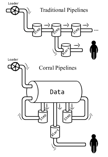
Figure 1: Data road-map in traditional pipeline architecture (upper panel) and Corral’s pipeline model (lower panel). In previous pipeline models data is being processed sequentially from one Step to the next one, with the possible scenario of parallel branching; while in the model proposed in this work Steps are independent entities that interact with a shared central data container. In both architectures data can be extracted when desired conditions are met, and shared at any time to users.

4.3 Some Words About Multiprocessing and Distributed Computing

As previously mentioned our project is built on top of a RDBMS, which by design can be accessed concurrently from a local or network computer. Every step accesses only the filtered part of the stream, so with minimum effort one can deploy the pipeline in one or more computers and run the steps in parallel. All the dangers of data corruption are avoided by the ACID (Atomicity, Consistency, Isolation and Durability) properties of the database transactions. This approach works well in most scenarios, but there are some unavoidable drawbacks, that arise for example in real-time processing, where consistency is less important than availability.Corral takes advantage of this technology to start a process for each Loader, Step or Alert within the pipeline, and allows interaction with the data stored in the database. If needed, groups of processes can be manually distributed on nodes of a cluster where the nodes will interact with the database remotely.

It is worth noting that any inter-processes direct communication is forbidden by design, and the only way to exchange messages is through the database.On this last particular point, the absolute isolation of the processes, is guaranteed by the MVC pattern.

4.4 Quality – Trustworthy Pipelines

One important requirement for a pipeline is the reliability of its results. A manual check of the data is virtually impossible when its volume scales to the TeraByte range. In our approach we suggest a simple unit testing approach to check the status of the stream before and after every Step, Loader or Alert.

Because tests are unitary, Corral guarantees the isolation of each test by creating and destroying the stream database before and after execution of the test. If you feed the stream with a sufficient amount of heterogeneous data you can check most of the pipeline’s functionality before the production stage. Finally we provide capabilities to create reports with all the structural and quality assurance information about the pipeline in convenient way, and a small tool to profile the CPU performance of the project.

4.4.1 Quality Assurance Index (QAI)

We recognize the need of a value to quantify the pipeline software quality. For example, using different estimators for the stability and maintainability of the code, we arrived at the following Quality Index:

$$QAI=\frac{\Theta\times\Lambda_{Cov}\times R_{PT}}{\gamma}$$

and $\gamma$ is a penalty factor defined as:

$$\gamma=\frac{1}{2}\times\left(1+exp\left(\frac{N_{SError}}{\tau\times N_{f}}\right)\right)$$

$\Theta$ is 1 if every test passes or 0 if any one fails, $R_{PT}$ is the ratio of tested processors (Loader, Steps and Alerts) to the total number of processors, $\Lambda_{Cov}$ the code coverage (between 0 and 1), $N_{SError}$ is the number of style errors, $\tau$ is the style tolerance, and $N_{f}$ is the number of files in the project. The number of test passes and failures are the unit-testing results, that provide a reproducible and updatable manner to decide whether your code is working as expected or not. The $\Theta$ factor is a critical parameter of the index, since it is discrete, and if a single unit test fails it will set the QAI to zero, in the spirit that if your own tests fail then no result is guaranteed to be reproducible. The $R_{PT}$ factor is a measure of how many of the different processing stages critical to the pipeline are being tested (a low value of this parameter should be interpreted as a need to write new tests for each pipeline stage). The $\Lambda_{Cov}$ factor shows the percentage of code that is being executed in the sum of every unit test; this displays the ”quality of the testing” (a low value should be interpreted as a need to write more extensive tests, and it may correlate with a low number of processors being tested, that is a low $R_{PT}$). $N_{NSerr}/(\tau\times N_{f})$ is the scaling factor for the exponential. It comprises the information regarding style errors, attenuated by a default or a user-defined tolerance $\tau$ times the number of files in the project $N_{f}$. The exponential function expresses the fact that a certain number of style errors isn’t critical, but after some point this seriously compromises the maintainability of the software project, and in this situation $\gamma$ strongly penalizes the quality index.The factor $1/2$ is a normalization constant, so that $QAI\in[0,1]$. This index aims to encode in a single figure of merit how well the pipeline meets the requirements specified by the user. We note that this index represents a confidence metric. Thus a pipeline could be completely functional even if every test fails, or if no tests are yet written for it. And in the opposite direction, the case where every test passes and the pipeline is delivering wrong or bogus results is possible.The $QAI$ index attempts to answer the question of pipeline reliability and whether a particular pipeline can be trustworthy. It should not be confused with the pipeline’s speed, capability, or any other performance metric.

4.4.2 Determining the default error tolerance in a python project

Corral, as earlier mentioned is written in Python, which offers a number of third party libraries for style validation. Code style in Python is standardized by the PEP 8 document. Flake8 is a style tool that allows the user to measure the number of style errors, that reflects the maintainability of the project.

For the $QAI$ measurement of Corral a key detail was in the determination of the amount of style errors developers tollerate as normal. For this we collected data from nearly $4000$ public Python source code files. The number of style errors was determined using Flake8 and the inter-quartile mean was determined as a measurement for $\tau$. A $\tau$ of $\sim 13$ was found. It is important to note that this value can be overridden by the user if a stronger QAI is required (Fig. 2).

Figure 2: Ideal test pass, and coverage QAI curves, with $N_{SErr}\in[0,40]$ for four values of $\tau$, for only one file. A damp in the error slope decay can be observed when $\tau$ is higher.

4.4.3 Quality and Structural reporting

Corral includes the ability to automatically generate documentation, creating a manual and quality reports in Markdown syntax that can be easily converted to a preferred format such as PDF (ISO., 2005), LaTeX (Lamport, 1994) or HTML (Price, 2000). A Class-Diagram (Booch et al., 2006) generation tool for the Models defined using Graphviz are also available for the pipelines created with Corral. We provide in Appendix A.4 an example of a pipeline (EXO) with an implementation of tests and the corresponding results of the QA report.

4.4.4 Profiling

Corral offers a deterministic tool for the performance analysis of CPU usage at a function level during the execution of unit tests. It is worth noting that in case a pipeline shows signs of lagging or slowing down, running a profiler over a unit test session can help locate bottlenecks. However for rigurous profiling, real data on real application runs should be used, instead of unit testing.

Another kind of profiling at the application level could be carried out manually using existing Python ecosystem tools such as memory_profiler (memory line level deterministic profiling), statsprof.py (statistic function level profiling), o line_profiler (line level deterministic) amongst other tools. We note that although some application level profiling tools are included or suggested, Corral was never intended to offer a system profiling tool. Nor does it claim to offer data base profiling, or I/O, energy profiling, network profiling, etc.

4.4.5 Final words about Corral quality

The framework does not contain any error backtrace concept, or retry attempts in processing. Each processor should be able to handle correctly the required information on its conditions. It is implicitly expected that the quality tools offered serve to unveil code errors as well.

If the pipeline’s developer achieves a high code coverage and is able to test enough data diversification, the possible software bugs can decrease substantially, up to 80% (Jeffries and Melnik, 2007).

5 Study case: A Simple Pipeline to Transform (x, y) Image Coordinates to world coordinates (RA, Dec)

A few examples are given below to illustrate each part of a toy model pipeline built over Corral. A more extended example can be found in appendix A and in the TOROS GitHub repository page https://github.com/toros-astro/toritos, where a fully functional astronomical image preprocessing pipeline is available.

We encourage the interested users to read the full Corral tutorial located at: http://corral.readthedocs.io

5.1 A Model example

In the following example a Model for an astronomical source is shown. It uses both $(x,y)$ and $(RA,Dec)$ coordinates and a field given for apparent magnitude. The identification field is automatically settled.

# this code is inside mypipeline/models.py
from corral import db

class PointSources(db.Model):
  "Model for star sources"
  __tablename__ = "PointSources"

  id = db.Column(
    db.Integer, primary_key=True)
  x = db.Column(db.Float, nullable=False)
  y = db.Column(db.Float, nullable=False)
  ra = db.Column(db.Float, nullable=True)
  dec = db.Column(db.Float, nullable=True)

  app_mag = db.Column(db.Float, nullable=False)

5.2 A Loader example

In the following example a Loader is shown, where the PointSource Model from above example is filled with new data. We note that the $(RA,Dec)$ fields in PointSource Model are allowed to be null, and therefore there is no need to set them a priori.

# this code is inside mypipeline/load.py
from astropy.io import ascii
from corral import run

from mypipeline import models

class Load(run.Loader):
  "Pipeline Loader"
  def setup(self):
    self.cat = ascii.read(
        ’point_sources_cat.dat’)

  def generate(self):
    for source in self.cat:
      src = models.PointSource()
      src.x = source[’x’]
      src.y = source[’y’]
      src.app_mag = source[’app_mag’])
      yield src

5.3 A Step example

An example Step is displayed below, where a simple data transformation is conducted. Where the step takes a set of sources and transforms their $(x,y)$ coordinates to $(RA,Dec)$: lines 10-12 show definitions for Class-level attributes, which are responsible for this query. The framework retrieves the data and serves it to the process method (line 14), which executes the relevant transformation and loads the data for each source.

# this code is inside mypipeline/step.py
from corral import run
from mypipeline import models

import convert_coord

class StepTransform(run.Step):
  "Step to transform from x,y to ra,dec"

  model = models.PointSource
  conditions = [model.ra == None,
                model.dec == None]

  def process(self, source):
    x = source.x
    y = source.y

    source.ra, source.dec = convert_coord(x, y)

5.4 Alert Example

In the example below an Alert is triggered when a state satisfies a particular condition of data in the stream. A group of communication channels are activated. In this particular case an email and an Astronomical Telegram (Rutledge, 1998) are posted whenever a point source is detected in the vicinity of $\textrm{Sgr A}^{*}$, near the center of the galaxy.

# this code is inside mypipeline/alert.py
from corral import run
from corral.run import endpoints as ep

from mypipeline import models

class AlertNearSgrA(run.Alert):

  model = models.PointSource
  conditions = [
    model.ra.between(266.4, 266.41),
    model.dec.between(-29.007, -29.008)]
  alert_to = [ep.Email(["sci1@sci.edu",
                        "sci2@sci.edu"]),
              ep.ATel()]

5.5 Running your Pipeline

As seen in the previous sections we define our protocol for the stream and the actions to be performed in order to covert the coordinates; but code is never defined to schedule the execution. Nevertheless applying the Corral MVC equivalent pattern guarantees that every loader and step is to be executed independently which means that both tasks run as long as there is data to work with. In every Step/Loader/Alert there is a guarantee of data consistency since each is attached to an SQLAlchemy session, and every task is linked to a database transaction. Since every SQL transaction is atomic, so the process is executed or fails, thus lowering the risk of data corruption in the stream.

Typically for a given pipeline with defined: Loader; Alert and Steps, the following output is produced:

$ python in_corral.py run-all
[mypipeline-INFO@2017-01-12 18:32:54,850]
    Executing Loader
    ’<class ’mypipeline.load.Load’>’
[mypipeline-INFO@2017-01-12 18:32:54,862]
    Executing Alert
    ’<class ’mypipeline.alert.AlertNearSgrA’>’
[mypipeline-INFO@2017-01-12 18:32:54,874]
    Executing Step
    ’<class ’mypipeline.load.StepTransform’>’
[mypipeline-INFO@2017-01-12 18:33:24,158]
    Done Alert
    ’<class ’mypipeline.alert.AlertNearSgrA’>’
[mypipeline-INFO@2017-01-12 18:34:57,158]
    Done Step
    ’<class ’mypipeline.load.StepTransform’>’
[mypipeline-INFO@2017-01-12 18:36:12,665]
    Done Loader
    ’<class ’mypipeline.load.Loader’>’ #1

It can be seen in the time stamps of the executions and task completions for the Loader, Alert and Steps; that there is no relevant ordering between them.

5.6 Checking The Pipeline Quality

5.6.1 Unit Testing

Following the cited guidelines of Feigenbaum (1983) who states that quality is a user defined specification agreement, it is necessary to make this explicit in kind in code that for Corral is achieved in a unit-test. Below an example is included showing a basic test case for our Step. The Corral test, feeds the stream with some user defined mock data, then runs the Step and finally checks if the result status of the stream meets the expected value.

# this code is inside mypipeline/tests.py
from corral import qa

from mypipeline import models, steps

import convert_coord

class TestTransform(qa.TestCase):
  "Test the StepTransform step"
  subject = steps.StepTransform

  def setup(self):
    src = models.PointSource(
      x=0, y=0, app_mag=0)
    self.ra, self.dec = convert_coord(0, 0)
    self.save(src)

  def validate(self):
    self.assertStreamHas(
      models.PointSource,
      models.PointSource.ra==self.ra,
      models.PointSource.dec==self.dec)
    self.assertStreamCount(
      1, models.PointSource)

As shown in lines 12-16 the setup() method is in charge of creating new data –whose transformed result is already known–, so then validate() asserts the outcome of StepTransform. This process would be repeated if more tests were defined, and an important caveat is that, mocked data streams are private to each unit test so will never collide producing unexpected results.

5.6.2 Quality Report and Profiling

Corral provides built-in functionalities to communicate quality assurance information:

1. create-doc: This command generates a Markdown version of an automatically generated manual for the pipeline. It includes information on Models, Loader, Steps, Alerts, and command line interface utilities, using docstrings from the code itself.

2. create-models-diagram: This creates a Models Class Diagram (Booch et al., 2006) in Graphviz dot format (Ellson et al., 2001).

3. qareport: Runs every test and Code Coverage evaluation, and uses this to create a Markdown document detailing the particular results of each testing stage, and finally calculates the QAI index outcome.

4. profile: Executes all existing tests and deploys an interactive web interface to evaluate the performance of different parts of the pipeline.

With these four commands the user can get a detailed report about structural status, as well a global measurement of quality level of the pipeline.

6 Corral: Under the hood

Put simply, Corral is a Pipeline environment that autoconfigures itself on each user command for which the following operations are exectued:

1. First of all in_corral.py inserts the path of settings.py into the environment variable Corral_SETTINGS_MODULE. With this simple action every Corral component knows where to find the pipeline’s configuration.

2. The command line parser is created, and commands provided by Corral are made available.

3. If the user asks for help (with the --help|-h flag) –or the requested command does not exist–, the help page is printed to screen.

4. Given a valid command, the line arguments are parsed so the requested action is identified, and set to be executed.

5. Based on the requested command, the framework would work in three DBMS modes:

   Mode in: The production DB is configured as the back-end to each model. This kind of configuration is used since in general commands require knowledge of the data stored in the stream.

   Mode test: The test DB is configured (by default in-memory DB is used). This mode is used by commands that require destructive operations over the database, eg test,coverage,profile

   Mode out: No database is configured. Some commands do not require any operations over the stream, like lsstep, used to list all the existing steps.

6. The command true logic is executed.

7. The teardown is executed for every connection.

8. Finally the python interpreter is shut down and the current error code is delivered to the operative system.

As mentioned the most basic functionality of Corral is to find files based in only one environment configuration. This brings to the developer clear rules to split the functionality in well defined and focused modules.

According to measured estimates, typically 1.5–2 s of overhead is required for any executed command, depending on the number of processes spawned. Almost 100% of the overhead is spent before the true command logic is executed. An interesting point to this is that the running mode of commands strongly affects the execution time (’out’ mode is much faster than ’test’ with in-memory database; and test is much faster than ’in’ mode). Other external factors causing potential bottlenecks that are worth mentioning are database location, I/O, Operating System configuration, or any hardware problems; although these should produce lack of performance not only to Corral but to any piece of software the user is executing.

7 Comparison with other pipeline frameworks

The two main differences between Corral and other similar projects are now explained. (A comparison of other alternatives is shown in Appendix B): First, to our knowledge Corral is the first implementations of a pipeline framework that uses MVC; and second the quality integration metrics that give an indication of the trustworthiness of the resulting pipeline.

The use of the MVC design standard imposes the following processing tasks (Loader, Steps and Alerts) result in a strong isolation condition: every processing stage only interacts with filtered data according to specific criteria with no bearing on information of the source or data destination. A major advantage of isolation is the natural parallelization of processing tasks since no ”race condition” is created. Regarding real-time processing this pattern can be inconvenient, since batches of data are processed asynchronously, leading to random ordering of data processing and writing onto the Database.

Corral features ”integration quality” utilities as an important tool set that builds confidence on the pipeline. This works when unit-tests are available for the current pipeline and in these cases Corral can automatically generate reports and metrics to quantify reliability. Corral was designed to optimize pipeline confidence in terms of some global notion of quality, which implies revision of data in each processing stage. Pelican is the only project integrating tools for pipeline testing, but does not include extra functionalities based on this concept. In many other aspects as depicted in appendix B, Corral is similar to other alternatives. A majority of these alternative also use Python as the programing language mainly in order to make use of its vast libraries for data access and manipulation, across multiple formats.

8 Real Pipelines Implemented on Corral

To date three pipelines have been implemented on Corral.

1. The TORITOS pipeline for image pre-processing. TORITOS is a pilot project for TOROS which employs a 16” telescope to take images in the Macón ridge. The pipeline is available at https://github.com/toros-astro/toritos.

2. Carpyncho is a Machine Learning facility, for the VVV (Minniti et al., 2010) survey data, specifically built to find variable stars in the Galactic Bulge and adjacent disk zone (Cabral et al., 2016).

3. A pipeline for synthetic data generation for machine learning training, focused on transient detection on survey images (Sánchez et al. 2017 in preparation).

9 Conclusions and Future Work

In this work a pipeline framework is presented that facilitates designing a parallel work flow for data multi processing. MVC design pattern was employed, that delivers a set of processing entities –Models, Steps, and Alerts– capable of carrying out a wide variety of scientific data pipeline tasks inside a concurrent scheduled environment. Last but not least, detailed quality and structural reports can be extracted and compared to the user’s predefined level of agreement to determine the pipeline trustworthiness and ultimately the validity of processed data.

Future work includes improvements on Corral’s performance by integrating the framework scheduler over distributed computing systems. This could run, for example, on top of Apache Hadoop, or Apache Spark, as these are the state of the art regarding data processing capability. Another possibility for the future is to replace the task scheduler that currently uses the module multiprocessing from the standard Python library, with Apache storm

Some other projects that could make use of this framework include Weak lensing analysis pipelines, Radio Telescope image generation and analysis, spectroscopic data analysis on star clusters and many more.

The capabilities of the presented framework can be a game-changer in isolated environments where hardware is operated remotely and resilience is an important requirement; and since it is straightforward, Corral can be used in a wide variety science cases. Anyone or any group interested in using Corral is invited to direct any questions, suggestions, feature request or advice at https://groups.google.com/forum/#!forum/corral-users-forum.

10 Acknowledgments

The authors would like to thank to their families and friends, the TOROS collaboration members for their ideas, and also IATE astronomers for useful comments and suggestions.

This work was partially supported by the Consejo Nacional de Investigaciones Científicas y Técnicas (CONICET, Argentina) and the Secretaría de Ciencia y Tecnología de la Universidad Nacional de Córdoba (SeCyT-UNC, Argentina). B.O.S., and J.B.C, are supported by a fellowship from CONICET. Some processing was acheived with Argentine VO (NOVA) infrustructure, for which the authors express their gratitude.

This research has made use of the http://adsabs.harvard.edu/, Cornell University xxx.arxiv.org repository, the Python programming language and SQLAlchemy library, other packages used can be found at Corral gihtub webpage.

References

Here we present two examples of pipeline development.

Appendix A A quick–start guide to creating a Corral pipeline

A.1 Installation

The recommended installation method for getting Corral running is using pip:

$ pip install -U corral-pipeline

Other methods are also possible, and are detailed in the online documentation.

A.2 Simple pipeline examples

Here we present a quick start guide to use Corral to set up a pipeline, with two simple examples.

The workflow for creating a simple pipeline can be summarized as follows (see also Fig. 3):

• Create the pipeline

• Define the models

• Create the database for the data

• Load the data

• Define the steps

• Run the pipeline

We show in what follows two simple examples of pipelines along with some relevant code that show the basics to get started with using Corral.

The first example uses the IRIS data, and is intended to compute some simple statistics. The IRIS flower data set (fis, ) is a commonly used multivariate data set that stores data from 3 species of the iris flower (”Setosa”, ”Virginica” and ”Versicolor”). In the following subsection we show how to implement a pipeline that reads the IRIS data, stores it in a database and perform some simple statistics.

A second example uses data from Exoplanet Data Explorer, which is an interactive web service to exploring data from the Exoplanet Orbit Database (Han et al., 2014), that stores a compilation of spectroscopic orbital parameters of exoplanets and stellar parameters of their host stars. In this example, we will construct a pipeline to store exoplanets data and perform some simple exploratory analysis. The pipeline to be created would be as follows:

• Download the data from exoplanets.org

• Update the database

• Create a scatter plot of planets period vs. mass

In both cases, the pipeline can be constructed using the Corral framework by performing the following operations:

• Create the pipeline, set the location of the data file and other configuration parameters in settings
  corral create my_pipeline

• Define the models for the data base. In this case, tell what kind of data will be stored in the database, set names, etc.

• Create the database for the data. This is accomplished according to the settings and the models.

• Load the data: read the CSV table and save it in the database.
  python in_corral.py load

• Define the steps: write the code to be applied to the data.

• Run the pipeline: this will read the data from the database and perform all the steps defined before.
  python in_corral.py run

• Output data can be obtained through Alerts.
  python in_corral.py check-alerts

In what follows we present a step–by–step guide to carry out this tasks.

Figure 3: Basic scheme of the workflow to build a pipeline using Corral

After installation, a pipeline can be created by running the command:

   $ corral create my_pipeline

which creates a file in_corral.py and a new directory ’my_pipeline’. The file in_corral.py is the access point to the pipeline, and allows commands to be executed inside the environment of the pipeline. The directory my_pipeline is the root directory for the pipeline, and the actual Python package for the project. Its name is the Python package name that can be used to import anything inside it (e.g. my_pipeline.models). The name my_pipeline can be replaced by IRIS or EXO, for our examples on IRIS data or exoplanet data, respectively. There are some files that are created within the project directory, each of them with a specific purpose within the Corral framework:

my_pipeline/__init__.py

An empty file that tells Python that this directory should be considered a Python package.

my_pipeline/pipeline.py

The suggested file to globally configure the pipeline on execution time.

my_pipeline/models.py

Contains the entities (or tables) that are stored in the pipeline’s database.

my_pipeline/load.py

Contains the Loader class. This would be the entry point for raw data to the pipeline stream, before going through any defined Steps.

my_pipeline/steps.py

Contains all pipeline steps.

my_pipeline/alerts.py

Contains the definitions of the Alerts, that offer custom communication channels to report expected results (a email for instance).

my_pipeline/commands.py

Used to add custom console commands, specific for the pipeline.

Each time a new pipeline is created, the first step is to perform the configuration by editing the file settings.py This file contains the variables that should be set in order to put the pipeline into work. In particular, it stores the location of the settings.py file:

PATH = os.path.abspath(os.path.dirname(__file__))

and also stores information about the locations of data files. For example, we can create the variable IRIS_PATH in the IRIS pipeline that stores the location of the data file containing the IRIS data, iris.csv

IRIS_PATH = os.path.join(PATH, "iris.csv")

This file contains 5 columns, listing the sepal length, sepal width, petal length, petal width and name of 150 samples if the IRIS flower from the original dataset (Fisher 1936).

For the exoplanets pipeline, we store the data in the file exoplanets.csv, which contains the following columns: name, period and mass of the planet; star–planet separation; distance to the host star; and mass, radius, effective temperature and metallicity of the star. This is a subset of data obtained from exoplanets.org. For this pipeline, the only modification in the settings.py file, with respect to the other example, is:

EXO_PATH = os.path.join(PATH, "exoplanets.csv")

Besides this basic configuration, the names of classes containing loaders, steps and alerts must be listed in the LOADER, STEPS and ALERTS variables, respectively. For example, for the IRIS pipeline we create 4 steps:

STEPS = [
    "pipeline.steps.StatisticsCreator",
    "pipeline.steps.SetosaStatistics",
    "pipeline.steps.VirginicaStatistics",
    "pipeline.steps.VersicolorStatistics"]

A.3 Processing of the IRIS data

As an essential part of the MVC pattern, the next step in preparing the pipeline is to define the models. The Model determines the structure of the data, and is defined in the models.py file.

We can create a model as a database which consists on two tables. The Flower table has 4 columns that store the sepal length and width, and the petal length and width, in the variables sepal_l, sepal_w, petal_l, and petal_w, respectively. The other table stores the name of the flower (Name). Each model is a class that inherits from db.model, so that Corral take these as tables in the database. Both tables are linked through their primary keys, which are added automatically when the database is created.

from corral import db

class Name(db.Model):

    __tablename__ = ’Name’

    id = db.Column(db.Integer, primary_key=True)
    name = db.Column(db.String(50), unique=True)

class Flower(db.Model):

    __tablename__ = ’Flower’

    id = db.Column(
        db.Integer, primary_key=True)

    name_id = db.Column(
        db.Integer, db.ForeignKey(’Name.id’),
        nullable=False)
    name = db.relationship(
        "Name", backref=db.backref("flowers"))
    sepal_l = db.Column(
        db.Float, nullable=False)
    sepal_w = db.Column(
        db.Float, nullable=False)
    petal_l = db.Column(
        db.Float, nullable=False)
    petal_w = db.Column(
        db.Float, nullable=False)

In the IRIS example, in order to compute a basic statistic (the mean) for each data column, an additional table must be created to store the results (and any other value that could be required). This table in the database is linked to the ”flowers” table by its primary key, which is generated automatically. It must be declared into the models.py file:

class Statistics(db.Model):

    __tablename__ = ’Statistics’

    id = db.Column(db.Integer, primary_key=True)
    name_id = db.Column(
        db.Integer, db.ForeignKey(’Name.id’),
        nullable=False, unique=True)
    name = db.relationship(
        "flowers", uselist=False,
        backref=db.backref("statistics"))

    mean_sepal_l = db.Column(
        db.Float, nullable=False)
    mean_sepal_w = db.Column(
        db.Float, nullable=False)
    mean_petal_l = db.Column(
        db.Float, nullable=False)
    mean_petal_w = db.Column(
        db.Float, nullable=False)

    def __repr__(self):
        return "<Statistics of ’{}’>".format(
            self.name.name)

Once the model is defined, the database is created with:

   $ python in_corral.py createdb

At this point the database does not contain any data, so the loaders must be used for that purpose. This is accomplished with the sentence

   $ python in_corral.py load

that uses the information set in the load.py file. This file contains the Loader class, which reads the data and save it to the database according to the model. The loader for this pipeline would be:

class Loader(run.Loader):

    def setup(self):
        self.fp = open(settings.IRIS_PATH)

    def get_name_instance(self, row):
        name = self.session.query(
            models.Name
        ).filter(
            models.Name.name == row["Name"]
        ).first()

        if name is None:
            name = models.Name(name=row["Name"])

            # we need to add the new
            # instance and save it
            self.save(name)
            self.session.commit()

        return name

    def store_observation(self, row, name):
        return models.Flower(
            name=name,
            sepal_l=row["SepalLength"],
            sepal_w=row["SepalWidth"],
            petal_l=row["PetalLength"],
            petal_w=row["PetalWidth"])

    def generate(self):
        for row in csv.DictReader(self.fp):
            name = self.get_name_instance(row)
            obs = self.store_observation(
                row, name)
            yield obs

    def teardown(self, *args):
        if self.fp and not self.fp.closed:
            self.fp.close()

In this example, setup is executed just before generate, and it is the best place to open the data file. On the other hand teardown runs after generate and uses information about their error state. The actual reading of each line in the data is split into two parts within generate: The method named get_name_instance receives the row as a parameter and returns a IRIS.models.Name instance referred to the name of such file (Iris-virginica, Iris-versicolor, or Iris-setosa). Every time a name is non existant this method must create a new one and store this model before returning it. Another method, store_observation, receives the row as a parameter, and also the instance of IRIS.models.Name just created by the previous model. This method just needs to return the instance and deliver it to the loader without saving it. Finally, the yields obs line within generate put the observation into the database through corral functionalities.

Once the data has been stored according to the model and is organized into the database, all the processing steps can be written as separate units into the steps.py file. Steps (and loaders) are controllers that do not need to run sequentially. Instead, a step will perform operations on the available data when the pipeline is run.

The Statistics class must be instantiated, for each different name on the flowers table, in the steps.py file using the definitions in models.py:

from . import models

class StatisticsCreator(run.Step):

    model = models.Name
    conditions = []

    def process(self, name):
        stats = self.session.query(
            models.Statistics
        ).filter(
            models.Statistics.name_id == name.id
        ).first()
        if stats is None:
            yield models.Statistics(
                name_id=name.id,
                mean_sepal_l=0.,
                mean_sepal_w=0.,
                mean_petal_l=0.,
                mean_petal_w=0.)

With the database ready to store the data, the mean can be computed through a specific process for each Name in flowers. For example, for the ”setosa” type:

class SetosaStatistics(run.Step):

    model = models.Statistics
    conditions = [
        models.Statistics.name.has(
            name="Iris-setosa"),
        models.Statistics.mean_sepal_l==0.]

    def process(self, stats):
        sepal_l, sepal_w = [], []
        petal_l, petal_w = [], []
        for obs in stats.name.flowers:
            sepal_l.append(obs.sepal_l)
            sepal_w.append(obs.sepal_w)
            petal_l.append(obs.petal_l)
            petal_w.append(obs.petal_w)
        stats.mean_sepal_l = sum(sepal_l)
        stats.mean_sepal_w = sum(sepal_w)
        stats.mean_petal_l = sum(petal_l)
        stats.mean_petal_w = sum(petal_w)
        stats.mean_sepal_l = (
            stats.mean.sepal_l/len(sepal_l))
        stats.mean_sepal_w = (
            stats.mean.sepal_w/len(sepal_w))
        stats.mean_petal_l = (
            stats.mean.petal_l/len(petal_l))
        stats.mean_petal_w = (
            stats.mean.petal_w/len(petal_w))

Similarly, the corresponding classes must be written for the other two Iris types. For the corral framework to be aware of the steps, they must be added in the settings.py file, as mentioned previously. Finally, the pipeline can be run using the following command line:

   $ python in_corral run

A.4 Processing of exoplanet data

The pipeline for the exoplanets has a different data structure, so its definition can be, for example:

class Planet(db.Model):

    __tablename__ = ’Planet’

    id = db.Column(
        db.Integer, primary_key=True)

    nomb = db.Column(db.Float, nullable=False)
    per = db.Column(db.Float, nullable=False)
    mass = db.Column(db.Float, nullable=False)
    sep = db.Column(db.Float, nullable=False)
    dist = db.Column(db.Float, nullable=False)
    mstar = db.Column(db.Float, nullable=False)
    rstar = db.Column(db.Float, nullable=False)
    teff = db.Column(db.Float, nullable=False)
    fe = db.Column(db.Float, nullable=False)

The load of the data is performed with just one table. Then, the Loader class contain the setup and teardown functions, which are the same than those in the IRIS example, except for the path to the data file, given in this case by settings.EXO_PATH. The generate function is:

import csv
from corral import run
from corral.conf import settings
from exo import models

class Loader(run.Loader):
    """Extract data from the ‘exoplanets.csv‘ and feed
    the stream of the pipeline.

    """

    def setup(self):
        # we open the file and assign it to
        # an instance variable
        self.fp = open(settings.EXO_PATH)

    def float_or_none(self, value):
        try:
            return float(value)
        except (TypeError, ValueError):
            return None

    def generate(self):
        # now we make use of "self.fp"
        # for the reader
        for row in csv.DictReader(self.fp):
            di = {
                ’name’: row[’NAME’],
                ’per’: self.float_or_none(
                    row[’PER’]),
                ’mass’: self.float_or_none(
                    row[’MASS’]),
                ’sep’: self.float_or_none(
                    row[’SEP’]),
                ’dist’: self.float_or_none(
                    row[’DIST’]),
                ’mstar’: self.float_or_none(
                    row[’MSTAR’]),
                ’rstar’: self.float_or_none(
                    row[’RSTAR’]),
                ’teff’: self.float_or_none(
                    row[’TEFF’]),
                ’fe’: self.float_or_none(
                    row[’FE’])}
            yield models.Planet(**di)

    def teardown(self, *args):
        # checking that the
        # file is really open
        if self.fp and not self.fp.closed:
            self.fp.close()

where the function Empty2None allows to deal with missing values, which is common in exoplanet data. This pipeline can also be extended by adding steps and alerts. For instance, a step can be configured to filter the dataset, compute correlation parameters, or apply machine learning techniques to discover clustering or perform classifications. If new planets are added to the data file, running the pipeline updates all the results previously computed. Also, the python environment allows to write alerts, which can be configured to produce plots, send the results by email or replace older versions in a webpage. Here we show an example of a step, which determines the list of planets in the habitable zone, and of an alert, which performs a scatter plot of mass and period of planets in the habiltable zone.

In order to add the list of planets in the habitable zone to the database, we create a new table as follows:

class HabitableZone(run.Step):
   __tablename__ = "HabitableZoneStats"

    id = db.Column(
        db.Integer, primary_key=True)

    planet_id = db.Column(
        db.Integer, db.ForeignKey(’Planet.id’),
        nullable=False)
    planet = db.relationship("Planet",
        backref=db.backref("hzones"))

    luminosity = db.Column(db.Float)
    radio_inner = db.Column(db.Float)
    radio_outer = db.Column(db.Float)

    in_habitable_zone = db.Column(db.Boolean)

Then, the step performs the search of planets that fulfill the requirement of being in the habitable zone. To that end, we compute the boundaries of the habitable zone as $rin=L/(1.1*L_{sun})$ and $rout=L/(0.53*L_{sun})$, and the luminosity as

$$L=4\pi R_{\ast}^{2}*\sigma T_{eff}^{4}$$ (1)

This is performed on the models.Planet model for the planets that have both the period and the mass measured in the dataset. All these planets that satisfy the condition of being in the habitable zone are then ingested to the data base on the HabitableZoneStats table.

from corral import run
import numpy as np
from astropy import units as u, constants as c
from . import models

STEFAN_BOLTZMANN = c.sigma_sb
SUN_LUMINOSITY = c.L_sun

class HabitableZone(run.Step):
    """Compute some statistics of the star of
    a given planet and then determines if is in
    their habitable zone.
    """

    model = models.Planet
    conditions = [model.rstar != None,
                  model.teff != None]

    def process(self, planet):
        # habitable zone of the host star
        Rstar  = (planet.rstar * u.solRad).to(’m’)
        Teff = planet.teff * u.K
        luminosity = (
            STEFAN_BOLTZMANN * 4 * np.pi *
            (Rstar ** 2) * (Teff ** 4))
        lratio = luminosity / SUN_LUMINOSITY
        rin = np.sqrt(lratio / 1.1)
        rout = np.sqrt(lratio / 0.53)

        in_hz = (
            planet.sep >= rin and
            planet.sep <= rout)
        return models.HabitableZoneStats(
            planet=planet,
            in_habitable_zone=in_hz,
            luminosity=lratio.value,
            radio_inner=rin.value,
            radio_outer=rout.value)

Finally, we show an alert that produces a scatter plot of planet mass vs. period:

class LogScatter(ep.EndPoint):

    def __init__(self, path, xfield, yfield,
                 title, **kwargs):
        self.path = path
        self.xfield = xfield
        self.yfield = yfield
        self.title = title
        self.kwargs = kwargs
        self._x, self._y = [], []

    def process(self, hz):
        planet = hz.planet
        x = getattr(planet, self.xfield)
        y = getattr(planet, self.yfield)
        if x and y:
            self._x.append(x)
            self._y.append(y)

    def teardown(self, *args):
        plt.scatter(
            p.log(self._x),
            np.log(self._y), **self.kwargs)
        plt.title(self.title)
        plt.legend(loc="best")
        plt.savefig(self.path)
        super(LogScatter, self).teardown(*args)

class PlotAlert(run.Alert):
    """Store a list of planets in habitable
    zone in a log file and also generate a
    period vs mass plot of this planets
    """

    model = models.HabitableZoneStats
    conditions = [
        model.in_habitable_zone == True]
    alert_to = [
        ep.File("in_habzone.log"),
        LogScatter(
            "in_habzone.png",
            xfield="per", yfield="mass",
            title="Period Vs Mass",
            marker="*")]

    def render_alert(self, now, ep, hz):
        planet = hz.planet
        data = []
        for fn in planet.__table__.c:
            data.append([fn.name,
            getattr(planet, fn.name)])
        fields = ", ".join(
            "{}={}".format(k, v) for k, v in data)
        return "[{}] {}\n".format(
            now.isoformat(),  fields)

In order to generate a report on the quality of this pipeline, we must perform some tests. In what follows, we show two tests that check for consistency in the data. The test in HabitableZoneTest creates an instance of a planet with $R_{\ast}=1$ and $T_{eff}=1$. This should produce a luminosity of $4*\pi*\sigma/L_{\odot}$, and should not be into the habitable zone. The test also accounts for the consistency of the boundary values, checking that the inner boundary is lesser than the outer boundary. Finally, it verifies that as a result of the step, just one entry on the HabitableZoneStats is produced.

class HabitableZoneTest(qa.TestCase):

    subject = steps.HabitableZone

    def setup(self):
        planet = models.Planet(
            name="foo", rstar=1, teff=1)
        self.save(planet)

    def validate(self):
        planet = self.session.query(
            models.Planet).first()
        hzone = planet.hzones[0]
        self.assertAlmostEquals(
            hzone.luminosity, 8.96223797571e-10)
        self.assertLess(
            hzone.radio_inner, hzone.radio_outer)
        self.assertFalse(hzone.in_habitable_zone)
        self.assertStreamCount(
            1, models.HabitableZoneStats)

The other test checks that in the case a planet does not have the two values that are required for the plot in the alert, no entry is generated on the HabitableZoneStats table.

class HabitableZoneNoRstarNoTeffTest(qa.TestCase):

    subject = steps.HabitableZone

    def setup(self):
        planet = models.Planet(name="foo")
        self.save(planet)

    def validate(self):
        self.assertStreamCount(0,
             models.HabitableZoneStats)

These tests produce a QA index of 27.31 per cent, and a qualification F with a 81.94 per cent coverage. It must be noticed that in order to improve the quality of this pipeline, more tests should be prepared. This example can be downloaded from the project repository. All the structural and quality documents can be found in GitHub pipeline repository in the following directions:

• Pipeline repository, https://github.com/toros-astro/corral_exoplanets

• QA report, https://github.com/toros-astro/corral_exoplanets/blob/master/exo/qareport.md

• Model class diagram, https://github.com/toros-astro/corral_exoplanets/blob/master/exo/models.png

• Pipeline documentation, https://github.com/toros-astro/corral_exoplanets/blob/master/exo/doc.md

Appendix B Comparative Table Between Several Pipeline Frameworks

In the following table we condense a collection of some of the most prominent pipeline implementations. Given a particular problem situation and resource constrain, it can be difficult to decide on a particular implementation of a pipeline and it would be even harder to test every pipeline framework available. See section 7 for a discussion.

Links

1. Corral: http://corral.readthedocs.io

2. Luigi: https://luigi.readthedocs.io

3. Airflow: http://airflow.apache.org/

4. Arvados: https://arvados.org

5. Azkaban: http://azkaban.github.io/azkaban

6. OPUS: http://www.stsci.edu/institute/software_hardware/opus/

7. Oozie: http://oozie.apache.org/

8. Kepler: https://kepler-project.org

9. Kira: https://github.com/BIDS/Kira/

10. Pelican: http://www.oerc.ox.ac.uk/~ska/pelican/

References

- (1) , . Fisher, R. A. (1936). The use of multiple measurements in taxonomic problems. Annals of Eugenics, 7, 179–188. URL: http://citeseer.comp.nus.edu.sg/context/3959/0.
- Abbott et al. (2016) Abbott, B. P. et al., 2016. Binary Black Hole Mergers in the First Advanced LIGO Observing Run. Physical Review X 6, 041015. doi:10.1103/PhysRevX.6.041015, arXiv:1606.04856.
- Abramovici et al. (1992) Abramovici, A. et al., 1992. LIGO - The Laser Interferometer Gravitational-Wave Observatory. Science 256, 325–333. doi:10.1126/science.256.5055.325.
- Axelrod et al. (2010) Axelrod, T., Kantor, J., Lupton, R., Pierfederici, F., 2010. An open source application framework for astronomical imaging pipelines, in: SPIE Astronomical Telescopes+ Instrumentation, International Society for Optics and Photonics. pp. 774015–774015.
- Bäumer et al. (1997) Bäumer, D., Gryczan, G., Knoll, R., Lilienthal, C., Riehle, D., Züllighoven, H., 1997. Framework development for large systems. Communications of the ACM 40, 52–59.
- Beroiz et al. (2016) Beroiz, M. et al., 2016. Results of optical follow-up observations of advanced LIGO triggers from O1 in the southern hemisphere, in: APS Meeting Abstracts.
- Booch et al. (2006) Booch, G., Rumbaugh, J., Jacobson, I., 2006. UML: guia do usuário. Elsevier Brasil.
- Bowman-Amuah (2004) Bowman-Amuah, M., 2004. Processing pipeline in a base services pattern environment. Google Patents. URL: http://www.google.com/patents/US6715145. uS Patent 6,715,145.
- Cabral et al. (2016) Cabral, J.B., Granitto, P.M., Gurovich, S., Minniti, D., 2016. Generación de features en la búsqueda de estrellas variables en el relevamiento astronómico vvv, in: Simposio Argentino de Inteligencia Artificial (ASAI 2016)-JAIIO 45 (Tres de Febrero, 2016).
- Cavuoti (2013) Cavuoti, S., 2013. Data-rich astronomy: mining synoptic sky surveys. arXiv:1304.6615 [astro-ph] URL: http://arxiv.org/abs/1304.6615. arXiv: 1304.6615.
- Coad (1992) Coad, P., 1992. Object-oriented patterns. Communications of the ACM 35, 152–159.
- Diaz et al. (2014) Diaz, M. C. et al., 2014. The TOROS Project, in: Wozniak, P.R., Graham, M.J., Mahabal, A.A., Seaman, R. (Eds.), The Third Hot-wiring the Transient Universe Workshop, pp. 225–229.
- Ellson et al. (2001) Ellson, J., Gansner, E., Koutsofios, L., North, S.C., Woodhull, G., 2001. Graphviz—open source graph drawing tools, in: International Symposium on Graph Drawing, Springer. pp. 483–484.
- Emerson et al. (2004) Emerson, J. P. et al., 2004. VISTA data flow system: overview, volume 5493. pp. 401–410. URL: http://dx.doi.org/10.1117/12.551582, doi:10.1117/12.551582.
- Feigenbaum (1983) Feigenbaum, A., 1983. Total quality control.
- Gorelick and Ozsvald (2014) Gorelick, M., Ozsvald, I., 2014. High Performance Python: Practical Performant Programming for Humans. ” O’Reilly Media, Inc.”.
- Gregg (2013) Gregg, B., 2013. Systems Performance: Enterprise and the Cloud. Pearson Education.
- Hadjiyska et al. (2013) Hadjiyska, E., Hughes, G., Lubin, P., Taylor, S., Hartong-Redden, R., Zierten, J., 2013. The transient optical sky survey data pipeline. New Astronomy 19, 99–108. doi:10.1016/j.newast.2012.08.006, arXiv:1210.1529.
- Han et al. (2014) Han, E., Wang, S.X., Wright, J.T., Feng, Y.K., Zhao, M., Fakhouri, O., Brown, J.I., Hancock, C., 2014. Exoplanet Orbit Database. II. Updates to Exoplanets.org. PASP 126, 827. doi:10.1086/678447, arXiv:1409.7709.
- Hughes et al. (2016) Hughes, A.L.H., Jain, K., Kholikov, S., the NISP Solar Interior Group, 2016. Gong classicmerge: Pipeline and product. ArXiv e-prints arXiv:1603.00836.
- ISO. (2005) ISO., 2005. Document Management: Electronic Document File Format for Long-term Preservation. ISO.
- Ivezic et al. (2008) Ivezic, Z., et al., for the LSST Collaboration, 2008. LSST: from Science Drivers to Reference Design and Anticipated Data Products. ArXiv e-prints arXiv:0805.2366.
- Jazayeri (2007) Jazayeri, M., 2007. Some trends in web application development, in: Future of Software Engineering, 2007. FOSE’07, IEEE. pp. 199–213.
- Jeffries and Melnik (2007) Jeffries, R., Melnik, G., 2007. Guest editors’ introduction: Tdd–the art of fearless programming. IEEE Software 24, 24–30.
- Klaus et al. (2010) Klaus, T. C. et al., 2010. Kepler Science Operations Center pipeline framework, volume 7740. pp. 774017–774017–12. URL: http://dx.doi.org/10.1117/12.856634, doi:10.1117/12.856634.
- Krasner et al. (1988) Krasner, G.E., Pope, S.T., others, 1988. A description of the model-view-controller user interface paradigm in the smalltalk-80 system. Journal of object oriented programming 1, 26–49.
- Kubánek et al. (2010) Kubánek, P., Nek, P., Kubá, Nek, P., 2010. RTS2 - The Remote Telescope System. Advances in Astronomy, Advances in Astronomy 2010, 2010, e902484. URL: http://www.hindawi.com/journals/aa/2010/902484/abs/,http://www.hindawi.com/journals/aa/2010/902484/abs/, doi:10.1155/2010/902484,10.1155/2010/902484.
- Kulkarni (2013) Kulkarni, S., 2013. The intermediate palomar transient factory (iptf) begins. The Astronomer’s Telegram 4807, 1.
- Lamport (1994) Lamport, L., 1994. Latex. Addison-Wesley.
- Magnier et al. (2006) Magnier, E., Kaiser, N., Chambers, K., 2006. The pan-starrs ps1 image processing pipeline, in: The Advanced Maui Optical and Space Surveillance Technologies Conference, volume 1. p. 50.
- Marx and Reyes (2015) Marx, R., Reyes, R.d.l., 2015. A Prototype for the Cherenkov Telescope Array Pipelines Framework: Modular Efficiency Simple System (MESS). arXiv:1509.01428 [astro-ph] URL: http://arxiv.org/abs/1509.01428. arXiv: 1509.01428.
- Masci et al. (2016) Masci, F. J. et al., 2016. The ipac image subtraction and discovery pipeline for the intermediate palomar transient factory. Publications of the Astronomical Society of the Pacific 129, 014002.
- Miller and Maloney (1963) Miller, J.C., Maloney, C.J., 1963. Systematic mistake analysis of digital computer programs. Communications of the ACM 6, 58–63.
- Minniti et al. (2010) Minniti, D. et al., 2010. Vista variables in the via lactea (vvv): The public eso near-ir variability survey of the milky way. New Astronomy 15, 433–443.
- Mohr et al. (2008) Mohr, J. J. et al., 2008. The dark energy survey data management system, in: SPIE Astronomical Telescopes+ Instrumentation, International Society for Optics and Photonics. pp. 70160L–70160L.
- Owens and Allen (2010) Owens, M., Allen, G., 2010. SQLite. Springer.
- Pedregosa et al. (2011) Pedregosa, F. et al., 2011. Scikit-learn: Machine learning in python. Journal of Machine Learning Research 12, 2825–2830.
- Pierro (2011) Pierro, M.D., 2011. web2py for Scientific Applications. Computing in Science & Engineering 13, 64–69. URL: http://scitation.aip.org/content/aip/journal/cise/13/2/10.1109/MCSE.2010.97, doi:10.1109/MCSE.2010.97.
- Price (2000) Price, R., 2000. Iso/iec 15445: 2000 (e). hypertext markup language.
- Renzi et al. (2009) Renzi, V. et al., 2009. Caracterización astronómica del sitio cordón macón en la provincia de salta. Boletin de la Asociacion Argentina de Astronomia La Plata Argentina 52, 285–288.
- Robitaille et al. (2013) Robitaille, T. P. et al., 2013. Astropy: A community python package for astronomy. Astronomy & Astrophysics 558, A33.
- Rose et al. (1995) Rose, J. et al., 1995. The opus pipeline: a partially object-oriented pipeline system, in: Astronomical Data Analysis Software and Systems IV, volume 77. p. 429.
- Roskind (2007) Roskind, J., 2007. The python profiler. URL http://docs. python. org/lib/profile. html .
- Rutledge (1998) Rutledge, R.E., 1998. The astronomer’s telegram: A web-based short-notice publication system for the professional astronomical community. Publications of the Astronomical Society of the Pacific 110, 754.
- (45) Schneider, S., . Statistical Profiling: An Analysis. URL: http://www.embedded.com/design/prototyping-and-development/4018371/Statistical-Profiling-An-Analysis.
- Thusoo et al. (2009) Thusoo, A. et al., 2009. Hive: a warehousing solution over a map-reduce framework. Proceedings of the VLDB Endowment 2, 1626–1629.
- Tollerud (2016) Tollerud, E., 2016. Jwst dadf (data analysis development forum) and photutils. psf, in: Python in Astronomy 2016.
- Tremblin et al. (2012) Tremblin, P., Schneider, N., Minier, V., Durand, G.A., Urban, J., 2012. Worldwide site comparison for submillimetre astronomy. Astronomy & Astrophysics 548, A65.
- Tucker et al. (2006) Tucker, D. L. et al., 2006. The Sloan Digital Sky Survey Monitor Telescope Pipeline. Astronomische Nachrichten 327, 821–843. URL: http://arxiv.org/abs/astro-ph/0608575, doi:10.1002/asna.200610655. arXiv: astro-ph/0608575.
- Van Der Walt et al. (2011) Van Der Walt, S., Colbert, S.C., Varoquaux, G., 2011. The numpy array: a structure for efficient numerical computation. Computing in Science & Engineering 13, 22–30.
- Zhang et al. (2016) Zhang, Z., Barbary, K., Nothaft, F.A., Sparks, E.R., Zahn, O., Franklin, M.J., Patterson, D.A., Perlmutter, S., 2016. Kira: Processing astronomy imagery using big data technology. IEEE Transactions on Big Data .