Abstract

Consider a surplus process which both of collected premium and payed claim size are two independent compound Poisson processes. This article derives two approximated formulas for the ruin probability of such surplus process, say double stochastic compound poisson process. More precisely, it provides two mixture exponential approximations for ruin probability of such double stochastic compound poisson process. Applications to long–term Bonus–Malus systems and a heavy-tiled claim size distribution have been given. Improvement of our findings compare to the Cramér-Lundberg upper bound has been given.
keywords: Ruin probability; Double Stochastic Compound Poisson Processes; Bonus–Malus system; Heavy-tailed distributions; Laplace transforms; Cramér-Lundberg upper bound.

1 Introduction

Consider double stochastic compound Poisson process

$$U_{t} = u+\sum_{i=1}^{N_{1}(t)}C_{i}-\sum_{j=1}^{N_{2}(t)}X_{j},$$ (1)

where $C_{1},C_{2},\cdots$ and $X_{1},X_{2},\cdots,$ respectively, are two independent i.i.d. random samples from independent random premium $C$ and random claim size $X$, two independent Poisson processes $N_{1}(t)$ and $N_{2}(t)$ (with intensity rates $\lambda_{1}$ and $\lambda_{2}$) are, respectively, stand for claims and purchase request processes, and $u$ represents initial wealth/reserve $u$ of the process. Moreover, suppose that non-negative and continuous random premium $C$ and claim $X,$ respectively, have density functions $f_{C}$ and $f_{X}$ with some additional properties to be discussed later (see Assumption 1 and Assumption 2).

The ruin probability for such process can be defined by

$$\psi(u) = p(T_{u}<\infty|U_{0}=u),$$ (2)

where $T_{u}$ is the hitting time, i.e., $T_{u}:=\inf\{t:~{}U_{t}\leq 0\}.$

Several authors studied the ruin probability under a stochastic income assumption such as the surplus process 1. For instance, Lappo (2004) provided an equation for the ruin probability of a surplus process which contains two compound Poisson processes. Rongming et al. (2007) considered a surplus process with random premium and geometric Lévy investments return process. They obtained an integro-differential equation for the ruin probability of such process. Lim & Qi (2009) considered a discrete-time surplus process and established an equation for the ultimate ruin probability. Moreover, they obtained an upper bound for the ruin probability and studied its properties via a simulation study. Under the compound binomial processes, Bao & Wang (2013) provided a difference equation and a defective renewal equation satisfied respectively by the expected discounted penalty function. Another version of the surplus compound binomial process has been studied by Yu (2013a). Yu (2013b) considered surplus process that both stochastic premium income and stochastic claims occurrence are driven by the Markovian regime-switching process. Then, he derived the Laplace transform of the time of ruin. Temnov (2014) provided a recursive formula similar to the Beekman convolution formula to evaluate the ruin probability for a stochastic premium surplus process. Landriault & Shi (2014) studied the finite-time ruin probability for double stochastic compound poisson processes whenever busy period follows a fluid flow model. Gatto & Baumgartner (2014a) using the saddlepoint method to derive an approximation for ruin probability of compound poisson risk process perturbed by diffusion. Gatto & Baumgartner (2014b) extended Gatto & Baumgartner (2014)’s findings to compound poisson risk process perturbed by a Wiener process with infinite time horizon. Cai & Yang (2014) provided an integro-differential equation for ruin probability of a compound Poisson surplus process perturbed by diffusion with debit interest.

It is well-known that, in the situation that, random premium $C$ and random claim size $X$ are two independent exponential random variables survival probability $\widetilde{\psi}(\cdot)$ can be found explicitly as an exponential function (Melnikov, 2011, Proposition 8.1). By an induction argument this fact can be readily generalized to situation that $C$ and $X$ are two independent mixture exponential random variables. In this situation, survival probability $\widetilde{\psi}(\cdot)$ appears as a mixture of some exponential functions. This article utilized this fact and approximates survival probability $\widetilde{\psi}(\cdot)$ appears as a mixture of some exponential functions. The rest of this article is organized as follows. Some mathematical background for the problem has been collected in Section 2. Section 3 provides the main contribution of this article. Applications of the results along with a and comparison with the Cramér-Lundberg upper bound have been given in Section 4.

2 Preliminaries

The following recalls the exponential type $T$ functions which plays a vital role in the rest of this article.

Definition 1.

An $L_{1}({\mathbb{R}})\cap L_{2}({\mathbb{R}})$ function $f$ is said to be of exponential type $T$ on ${\mathbb{C}}$ if there are positive constants $M$ and $T$ such that $|f(\omega)|\leq M\exp\{T|\omega|\},$ for $\omega\in{\mathbb{C}}.$

The Fourier transforms of exponential type functions are continuous functions which are infinitely differentiable everywhere and are given by a Taylor series expansion over every compact interval, see Champeney (1987, page 77) and Walnut (2002, page 81). The Fourier transform to exponential type functions are also called band-limited functions, see Bracewell (2000, page 119) for more details on band-limited functions. The well-known Paley-Wiener theorem states that the Fourier transform of an $L_{2}({\mathbb{R}})$ function vanishes outside of an interval $[-T,T],$ if and only if the function is an entire function of exponential type $T$, see Dym & McKean (1972, page 158) for more details. We also need one form of the half-line version of the Paley-Wiener theorem, namely that if a function in $f\in L_{2}({\mathbb{R}})$ vanishes on the left half-line, then its corresponding Fourier transform $\hat{f}$ is holomorphic and uniformly bounded in the upper half plane. Ablowitz & Fokas (1990 §4).

We also have need of the theory of residues for meromorphic functions. Briefly, $\mbox{Res}(f,z_{i})$ is the coefficient of $\frac{1}{z-z_{i}}$ in the Laurent series expansion of $f$ around $z_{i}.$ It is possible to define Laurent series about the point $z_{i}=\infty$, and hence it is possible to define a residue at infinity, $\mbox{Res}(f,\infty).$ The importance of the theory of residues probably rests on two facts: many integrals can be evaluated in terms of a sum of residues, and at poles of finite order residues can be evaluated efficiently by formulas:

$$\mbox{Res}(f,z_{0})=\frac{1}{(m-1)!}\lim_{s\rightarrow z_{0}}\left(\frac{d}{ds}\right)^{m-1}\!\!\!\!\!\!\!\!\!(s-z_{0})^{m}f(s),$$

where $m$ is the order of the pole, see for example Ablowitz & Fokas (1990 §4).

The following explores the Laplace transform of a function that behaves like an exponential function about zero.

Lemma 1.

Suppose $f(\cdot)$ is an exponential type function which behaves like an exponential function about zero, i.e., $f(\epsilon)=\alpha_{0}e^{-\beta_{0}\epsilon},$ where $\alpha_{0}$ and $\beta_{0}$ are two given positive numbers. Then, the Laplace transform $f(t+a)$ is

$$\mathcal{L}(f(t+a);t;s) = e^{sa}\mathcal{L}(f(t);t;s)-\frac{\alpha_{0}}{s+\beta_{0}}\left(e^{as}-e^{-a\beta_{0}}\right).$$ (3)

Proof. Suppose $f$ is of exponential type $T,$ the Taylor series expansion for $f(t+a)$ is

$$f(t+a)=\sum_{0}^{\infty}\frac{a^{k}}{k!}f^{(k)}(t),$$

where $f^{(k)}(\cdot)$ stands for the $k^{\hbox{th}}$ derivative of $f(\cdot).$

Using the Weierstrass M-test along with properties of exponential type function (i.e., $|f^{(k)}(t)|\leq|T|^{k}\|f\|_{\infty}.$). One may conclude that the above Taylor series converges uniformly with respect to both $a\in{\mathbb{C}}$ and $t\in{\mathbb{R}}.$ The uniform convergence justifies the following taking term-by-term Laplace transform.

$$\mathcal{L}(f(t+a);t;s) = \mathcal{L}(f(t);t;s)+\sum_{k=1}^{\infty}\frac{a^{k}}{k!}\mathcal{L}(f^{(k)}(t);t;s)$$

$$= \mathcal{L}(f(t);t;s)\left[1+\sum_{k=1}^{\infty}\frac{(as)^{k}}{k!}\right]-\sum_{k=1}^{\infty}\frac{a^{k}}{k!}\sum_{j=0}^{k-1}s^{j}f^{(k-j-1)}(0)$$

$$= e^{as}\mathcal{L}(f(t);t;s)-\sum_{k=1}^{\infty}\frac{a^{k}}{k!}\sum_{j=0}^{k-1}s^{j}\alpha_{0}(-\beta_{0})^{k-j-1}$$

$$= e^{as}\mathcal{L}(f(t);t;s)-\frac{\alpha_{0}}{s+\beta_{0}}\left(e^{as}-e^{-a\beta_{0}}\right),$$

where the second equality arrived from an application of the Laplace transform of a derivative, see Schiff (1999) for more details. $\square$

We consider a class of random variables with their corresponding density/probability functions and moment generating functions satisfy the following two assumptions:

Assumption 1.

Their density/probability and survival functions are exponential type functions, twice (continuously) differentiable, and bounded on ${\mathbb{R}}^{+};$

Assumption 2.

Their moment generating functions are or can be extended to a meromorphic function on ${\mathbb{C}}.$

Exponential, mixture exponential, Erlang, Pareto (with finite mean), normal, mixture normal, lognormal, etc are some distributions that satisfy Assumption1 (Cai, 2004) while Assumption 2 holds for most of the common distributions, such as binomial, negative binomial, poisson, uniform, normal, chi-squared (with an even degree of freedom), gamma (with integer shape parameter), laplace, etc. On the other hand, several nonmeromorphic moment generating functions can be analytically continued to a meromorphic functions. Geometric and Multinomial distributions are two examples which have nonmeromorphic moment generating functions but their moment generating functions can be analytically continued to a meromorphic function, see Kucerovsky & Payandeh (2014) and Sasv’ri (2013, §3.3) for more details.

By conditioning of the survival probability $\widetilde{\psi}(\cdot)$ of surplus process 1 on the first arriving premium and claim along with properties of compound Poisson process. One may derive the following integro-differential equation for survival probability $\widetilde{\psi}(\cdot)$ of surplus process 1, proof may be found in Rongming et al. (2007), Melnikov (2011, Theorem 8.1), among others.

$$-(\lambda_{1}+\lambda_{2})\widetilde{\psi}(u)+\lambda_{1}E(\widetilde{\psi}(u+C))+\lambda_{2}\int_{0}^{u}\widetilde{\psi}(u-x)f_{X}(x)dx=0,$$ (4)

where $\lim_{u\rightarrow\infty}\widetilde{\psi}(u)=1$ and two random premium $C$ and claim size $X$ satisfy assumptions Assumption 1 and Assumption 2.

In the situation that, $C$ and $X$ are two independent exponential random variables with rates $\mu_{1}$ and $\mu_{2},$ respectively. Then, survival probability can be found explicitly as $\widetilde{\psi}(u)=Ae^{-Bu},$ where $A:=(\mu_{1}+\mu_{2})\lambda_{2}/(\lambda_{1}+\lambda_{2})$ and $B:=(\mu_{1}\lambda_{1}-\mu_{2}\lambda_{2})/(\lambda_{1}+\lambda_{2}),$ see Melnikov (2011, Proposition 8.1) for more details. This fact can be generalized for situation that $C$ and $X$ are two independent mixture exponential random variables.

Hereafter now, we assume for very small surplus/reserve, say $u=\epsilon,$ survival probability behaves like an exponential function, i.e.,

Assumption 3.

For very small surplus/reserve $u=\epsilon$ survival probability behaves like $\widetilde{\psi}(\epsilon)=\alpha_{0}e^{-\beta_{0}u},$

where two positive numbers $\alpha_{0}$ and $\beta_{0}$ have to be determined. The above assumption can be explained by the above observation along with the fact that a given density/probability function can be approximated, with some degree of accuracy, by a mixture exponential distribution.

Coefficient $\beta_{0}$ in Assumption 3 can be found either by integro-differential Equation 4 and letting $u\rightarrow\infty$ or the fact that $\lim_{u\rightarrow\infty}\psi(u)e^{Ru}=c\in(0,1),$ where adjustment coefficient $R$ is positive solution of $\lambda_{1}M_{C}(R)+\lambda_{2}M_{X}(-R)=\lambda_{1}+\lambda_{2}$ (Kaas, et al., Page 112), see Proposition 2 for more details. While coefficient $\alpha_{0}$ cannot be found using integro-differential Equation 4 or other theoretical assumptions on ruin probability. Therefore, analogue to situation that $C$ and $X$ are two independent exponential random variables, we set $\alpha_{0}:=(1/E(C)+1/E(X))\lambda_{2}/(\lambda_{1}+\lambda_{2}).$

3 Main results

This section utilizes integro-differential Equation 4 to derive two approximate formulas for the ruin probability of a double stochastic compound Poisson process. 4. We seek an analytical solution $\widetilde{\psi}(\cdot)$ which is an exponential type function. In the other word, we assume:

Assumption 4.

$|\widetilde{\psi}(\omega)|\leq Me^{T|\omega|},~{}\omega\in{\mathbb{C}},$ for some real numbers $M$ and $T$ in ${\mathbb{R}}.$

If this assumption is not met, as might be the case if, for example, there are point masses in $\psi(\cdot),$ our methods may still result in a formal solution that can be verified by substitution into integro-differential Equation 4.

The following from provides an explicit expression for the ruin probability of a double stochastic compound Poisson process in an analytical model.

Theorem 1.

Suppose $U_{t}$ represents double stochastic compound Poisson process 1 which their random claim size $X$ and random premium $C$ satisfy Assumption 1 and Assumption 2. Moreover, suppose that survival probability $\widetilde{\psi}(\cdot)$ satisfies Assumption 3 and Assumption 4. Then,

i)

the Laplace transform of the ruin probability $\psi(\cdot)$ satisfies

$$\mathcal{L}(\psi(u);u,s) = \frac{N(s)}{s(s+\beta_{0})D(s)};$$ (5)

ii)

poles of $\frac{N(s)}{s(s+\beta_{0})D(s)},$ say $z_{j},$ can be represented as $z_{j}:=-a_{j}\pm ib_{j},$ where $a_{j}>0;$

iii)

There is at most one simple pole on the negative real axis,

where $D(s):=-\lambda_{1}-\lambda_{2}+\lambda_{1}M_{C}(s)+\lambda_{2}M_{X}(-s),$ $N(s):=(s+\beta_{0})D(s)-s\lambda_{1}\alpha_{0}(M_{C}(s)-M_{C}(-\beta_{0})),$ and $M_{C}(\cdot)$ and $M_{X}(\cdot)$ represent moment generating functions of $C$ and $X,$ respectively.

Proof. Taking a Laplace transform from integro-differential Equation 4 with an application of Lemma 1 complete part (i). For part (ii) observe that: by Assumption 3 and the Paley-Wiener theorem, we may conclude that an expression $g(s):=\frac{N(s)}{s(s+\beta_{0})D(s)}$ is holomorphic and uniformly bounded in the right-half plane. Therefore, $g(s)$ has no poles at any $z\in{\mathbb{C}}$ with non-negative real part. On the other hand, since $\psi(\cdot)$ is real-valued function, its corresponding Laplace transform is real everywhere on the real line (except possibly at poles) and hence by the Schwartz reflection principle,

$$\overline{\left(\frac{N(s)}{s(s+\beta_{0})D(s)}\right)}=\frac{N(\overline{s})}{\overline{s}(\overline{s}+\beta_{0})D(\overline{s})}.$$

Therefore, poles of $g(s)$ are located at $z_{j}:=-a_{j}\pm ib_{j}.$ To establish $a_{j}>0,$ observe that if there is a pole at some $z_{i}\in{\mathbb{C}},$ then there is also a pole at the complex conjugate, $\overline{z_{i}}.$ On the other hand, since $D(s)$ is a convex (concave up) function on the real line, it can have at most two zeros on the real line. Moreover, $D(s)$ has a zero at the origin, so there can be at most one other zero of $D(s)$ on the real line, necessarily located on the negative real line. For part (iii) observe that a simple pole for $g(s)$ on the negative real axis can be $-\beta_{0}.$ $\square$

Using the above theorem, one need only consider the roots of $D(s)=0,$ which are completely determined by the moment generating functions, random claim size $X,$ and random random premium $C,$ say respectively $M_{X}(\cdot)$ and $M_{C}(\cdot).$ Residues at simple poles are particularly easy to evaluate, and the case of simple poles is the generic case. If there are finitely many poles and all are of finite order, they may be made to be simple poles by an infinitesimal perturbation of the problem. Thus the following result is of practical importance. The condition that appears below, of the derivatives being non-zero, is more or less equivalent to all the zeros of $D(s)$ being simple zeros:

Corollary 1.

Under the same conditions as in Theorem 1, we then have that the ruin probability $\psi(\cdot)$ is

$$\psi(u) \approx \sum_{D(z_{i})=0,\,\Re(z_{i})<0}\frac{N(z_{i})}{z_{i}(z_{i}+\beta_{0})D^{\prime}(z_{i})}e^{z_{i}u}.$$

whenever the derivatives that appear are all non-zero.

Proof. The residue of $N(s)/(s(s+\beta_{0})D(s))$ at a simple zero $z_{i}$ of $D(s)$ is

$$\lim_{s\rightarrow z_{i}}\frac{(s-z_{i})N(s)}{s(s+\beta_{0})D(s)}=\frac{N(z_{i})}{z_{i}(z_{i}+\beta_{0})D^{\prime}(z_{i})}.$$

Conversely, if $D^{\prime}(s)$ is nonzero at a zero of $D(s)$ then this zero is a simple zero, and $N(s)/(s(s+\beta_{0})D(s))$ has at most a simple pole (as the zero is assumed to have negative real part). $\square$

Since the ruin probability is real and non-negative, and since the poles come in pairs, we can draw some further conclusions about the structure of the expression for $\psi(\cdot).$

Proposition 1.

Under the same conditions as in Theorem 1. The ruin probability $\psi(u)$ can be simplified by a finite sum of the form

$$\psi(u) \approx \alpha_{0}e^{-c_{0}u}+\sum_{i}A_{i}e^{-c_{i}u}\cos(d_{i}u)+\sum_{i}B_{i}e^{c_{i}u}\sin(d_{i}u),$$ (6)

where $c_{i}$ and $d_{i}$ are, respectively, real and imaginary parts of the roots of $D(s)=0$ and $A_{i},$ $B_{i}$ are real numbers evaluated by substituting 6 in Equation 4.

Proof. We have the above general form of a sum involving trigonometric functions and exponentials comes directly from Theorem 1, plus the fact that the poles come in pairs (Theorem 1.) The $b_{i}$ are the imaginary parts of the roots, and the $a_{i}$ are the real parts. Theorem 1 moreover tells us that there is at most one root on the negative real axis. Since the ruin probability must remain non-negative for large $u,$ but must vanish at infinity, it follows that the exponential corresponding to this purely real root must be the dominant term for large $u,$ and thus the purely real root is negative, nonzero, and is to the right of all the complex roots. $\square$

Remark 1.

It is a corollary of the proof above that under our conditions there does always exist a unique negative and nonzero real root of $D(s).$

Corollary 2.

Under the same conditions as in Theorem 1, and also assuming $D(s)/s=0$ has only a simple non-zero root at $z_{1},$ then, the ruin probability is given by

$$\psi(u) \approx \frac{\lambda_{2}}{\lambda_{1}+\lambda_{2}-\lambda_{1}M_{C}(z_{1})}e^{z_{1}u},$$

where $M_{C}(z_{1})$ stands for the moment generating function of the random variable $C$ at $z_{1}.$

Proof. Substituting $u=0$ in Equation 4, one may conclude that

$$\alpha_{0} := \psi(0)$$

$$= \frac{\lambda_{1}}{\lambda_{1}+\lambda_{2}}E(\psi(C))+\frac{\lambda_{2}}{\lambda_{1}+\lambda_{2}}$$

$$= \frac{\lambda_{1}}{\lambda_{1}+\lambda_{2}}\frac{N(z_{1})}{-z_{1}D^{\prime}(z_{1})}M_{C}(z_{1})+\frac{\lambda_{2}}{\lambda_{1}+\lambda_{2}}$$

$$= \frac{\lambda_{1}}{\lambda_{1}+\lambda_{2}}\alpha_{0}M_{C}(z_{1})+\frac{\lambda_{2}}{\lambda_{1}+\lambda_{2}},$$

where two last equalities arrive from double applications of Corollary 1, with simple non-zero root $z_{1}$ at $u=0.$ $\square$

In general, the moment generating function of a distribution, when it exists, will grow rapidly as we move to the right on the real axis, but decreases along the negative real axis, and decreases along the imaginary axis (because there it is the characteristic function). Thus, it is reasonable to expect that $M_{C}(z_{k})$ will be small for the off-axis roots of $D(s)$, since these roots are located in the second and third quadrants of the complex plane. Furthermore, since the moment generating function oscillates in the off-axis direction, sums involving the off-axis roots are likely to be quite small due to cancellations. If this is the case, then we can hope to approximate by neglecting the sum involving off-axis roots roots in the above calculation. We thus obtain the following approximation result.

Proposition 2.

. Under the same conditions as in Theorem 1, then the ruin probability $\psi(\cdot)$ about the origin can be approximated by one of the following exponential functions.

i)

If equation $D(s)=0$ has unique strictly negative real root, say $z_{1},$

$$\psi(\epsilon) \approx \frac{\lambda_{2}}{\lambda_{1}+\lambda_{2}-\lambda_{1}M_{C}(z_{1})}e^{z_{1}\epsilon};$$

ii)

If $\lambda_{1}E(C)\geq\lambda_{2}E(X)$

$$\psi(\epsilon) \approx \frac{E(C)+E(X)}{E(C)E(X)(\lambda_{1}+\lambda_{2})}e^{-\beta_{0}\epsilon};$$

iii)

$$\psi(\epsilon) \approx \frac{E(C)+E(X)}{E(C)E(X)(\lambda_{1}+\lambda_{2})}e^{-R\epsilon},$$

where $\beta_{0}$ is positive solution of $\lambda_{1}M_{C}(-\beta_{0})+\lambda_{2}M_{X}(\beta_{0})=\lambda_{1}+\lambda_{2}$ and adjustment coefficient $R$ is positive solution of $\lambda_{1}M_{C}(R)+\lambda_{2}M_{X}(-R)=\lambda_{1}+\lambda_{2}.$

Proof. Part (i) arrives by an application of Corollary 2. For part (ii) observe that substituting an exponential function $\alpha_{0}e^{-\beta_{0}u}$ into integro-differential Equation 4 and letting $u\rightarrow\infty.$ One may obtain equation $\lambda_{1}M_{C}(-\beta_{0})+\lambda_{2}M_{X}(\beta_{0})=\lambda_{1}+\lambda_{2}.$ Now, set $h(\beta_{0}):=\lambda_{1}M_{C}(-\beta_{0})+\lambda_{2}M_{X}(\beta_{0}).$ Using assumption on random premium $C$ and random claim size $X,$ one may conclude that $h(0)=\lambda_{1}+\lambda_{2},$ $\lim_{\beta_{0}\rightarrow\infty}h(\beta_{0})=\infty,$ $\lim_{\beta_{0}\rightarrow\infty}h^{\prime}(\beta_{0})=-\lambda_{1}E(C)+\lambda_{2}E(X)\leq 0,$ and $h^{\prime\prime}(\beta_{0})\geq 0.$ Therefore, the above equation has a unique positive solution in $\beta_{0}.$ Part (iii) arrives by an application of the fact that $\lim_{u\rightarrow\infty}\psi(u)e^{Ru}=c\in(0,1),$ (Kaas, et al., Page 112). Coefficient $\alpha_{0}$ for both parts (ii & iii) cannot be found using integro-differential Equation 4 or other theoretical assumptions on ruin probability. Therefore, analogue to situation that $C$ and $X$ are two independent exponential random variables, we set $\alpha_{0}:=(1/E(C)+1/E(X))\lambda_{2}/(\lambda_{1}+\lambda_{2}).$ $\square$

Residues at simple poles are particularly easy to evaluate, and the case of simple poles is the generic case. If there are finitely many (finite order) poles. They may be made to be simple poles by an infinitesimal perturbation of the problem. Therefore, an approximation for the ruin probability can be obtained by assuming all roots of $D(s)=0$ are simple. The following theorem improves accuracy of approximation result given by Theorem 1 whenever $D(s)=0$ has finitely many simple zeros.

Theorem 2.

Supposing that under the conditions of the above result, $D(s)$ has finitely many roots in the left half-plane. Then, $\psi(u)\approx\sum A_{i}e^{z_{i}u},$ where $A_{i}$ can be found out by the following linear system of equations

$$A_{j}=\frac{1}{\lambda_{2}z_{j}M^{\prime}_{X}(-z_{j})}\left(\lambda_{2}M_{X}(-z_{j})-\lambda_{2}+z_{j}\sum_{i\neq j}\frac{A_{i}}{z_{j}-z_{i}}\left(\lambda_{1}+\lambda_{2}-\lambda_{1}M_{C}(z_{i})-\lambda_{2}M_{X}(-z_{j})\right)\right).$$ (7)

Proof. Roots of $D(s)=0$ may be made to be simple poles by an infinitesimal perturbation of the problem. Therefore, $D(\cdot)$ has finitely many simple roots, $z_{i}$, we have by Lemma 1 and Proposition 1 that $\psi(u)\approx\sum A_{i}e^{z_{i}u}.$ Substituting $\psi(u)\approx\sum A_{i}e^{z_{i}u}$ into Equation 4 and taking the Laplace transform, we obtain

$$-(\lambda_{1}+\lambda_{2})\left(\frac{1}{s}-\sum_{i}\frac{A_{i}}{z_{j}-z_{i}}\right)+\lambda_{1}\left(\frac{1}{s}-\sum_{i}\frac{A_{i}}{z_{j}-z_{i}}M_{C}(z_{i})\right)+\lambda_{2}\left(\frac{1}{s}-\sum_{i}\frac{A_{i}}{z_{j}-z_{i}}\right)M_{X}(-s) = 0.$$

The desired proof arrives by setting $s=z_{j}$ along with an application of the $l^{\prime}H\hat{o}pital^{\prime}$s rule. $\square$

It is clear from the above that the solution obtained is in fact unique. The only further point to mention with respect to the above theorem that since we now are dealing with approximations, it could happen that the sum $\sum A_{i}e^{z_{i}u}$ obtained as in Theorem 2 is not quite real or not quite non-negative, so we adjust it in the above by taking the real part and then the floor with zero. The amount by which the sum $\sum A_{i}e^{z_{i}u}$ fails to be real and non-negative can be taken as a practical indication of the amount of error in the approximation. Normally, one would pick the complex zeros that are closest to the real root of $D(s),$ aiming to ensure that the complex moment function $M_{C}(z)$ has quite small absolute value at the zeros that have been neglected. Moreover, the set of roots chosen should be closed under complex conjugation, meaning that if $a+ib$ is in the set of roots, then $a-ib$ should also be in the set of roots.

It would be worthwhile mentioning that, the ruin probability may be impacted by different ways of adjustment (i.e., adjusting either $\psi(u)$ or complex roots). Sensitivity of such adjustment should be investigated and managed by the amount of error which obtained by substituting adjusted $\psi(\cdot)$ into Equation 4.

The following section is devoted to applications of Corollary 2 and Theorem 2.

4 Applications

In the most of practical application the ruin probability of surplus process 1 has been approximated by the Cramér-Lundberg upper bound $e^{-Ru},$ where adjustment coefficient $R$ is positive solution of $\lambda_{1}M_{C}(R)+\lambda_{2}M_{X}(-R)=\lambda_{1}+\lambda_{2}.$ Certainly, $-R$ is one of solution of our equation $D(s)=0.$ Practical implementation of the above findings along with a comparison with the well-known Cramér-Lundberg upper bound have been given in the following examples. Example 1 considers a situation that equation $D(s)=0$ has just one simple non-positive solution. In this situation our method improves the Cramér-Lundberg upper bound by a constant coefficient. While in the Example 2 that equation $D(s)=0$ has more than one simple non-positive root, our method provides a significant improvement on the Cramér-Lundberg upper bound.

Example 1.

Suppose an insurance company plans to charge its policyholders based upon their risks (such insurance systems well known as Bonus–Malus systems). Moreover suppose that the insurance company considers three different scenarios with 5, 10, and 20 premiums’ values such that under all of these scenarios expected revenue of the company stay the same by selling an insurance contract. Based upon a statistical investigation an actuary suggested the following premium values and probability that a given policyholder falls in a given level, say ${\bf\pi},$ of each scenario.

Table 1: Premiums values ${\bf C}$ and probability that a given policyholder falls in a given level for such three scenarios.
Scenario (number of its levels) ${\bf\pi}$ Premium value ${\bf C}$ S1 (with 5 levels) $\pi_{i}\equiv 0.2$ (0.6, 1, 1.4, 1.8, 2.2) S2 (with 10 levels) $\pi_{i}\equiv 0.1$ (0.4, 0.8, 1, 1.2, 1.4, 1.5, 1.7, 1.8, 2, 2.2) S3 (with 20 levels) $\pi_{i}\equiv 0.05$ (0.4, 0.5, 0.6, 0.7, 0.8, 0.9, 1, 1.1, 1.2, 1.3, – – 1.4, 1.5, 1.6, 1.7, 1.8, 1.9, 2.1, 2.2, 2.6, 2.7)

Moreover, suppose that the number of sold contracts, $N_{1}(t),$ and number of arrived claims, $N_{2}(t),$ are two independent Poisson processes with intensity $\lambda_{1}=18$ and $\lambda_{2}=11$ and claim size distributions given by Table 2.

It is easy to show that, for all cases, equation $D(s)=0$ has just one simple non-positive root. Using results of Corollary 2, one may evaluate the ruin probability in an exact mode. The ruin probability (as well as the Cramér-Lundberg upper bound) for such three different scenarios have been given by Table 2.

Table 2: The ruin probability and Cramér-Lundberg upper bound for the above three scenarios under different claim size distributions.
Scenario (number of its levels) Claim size distribution Scenario 1 (5) Scenario 2 (10) Scenario 3 (20) Gamma(1,3) $\psi(u)=0.313e^{-1.760u}$ $\psi(u)=0.312e^{-1.759u}$ $\psi(u)=0.280e^{-1.746u}$ $(\psi(u)\leq e^{-1.760u})$ $(\psi(u)\leq e^{-1.759u})$ $(\psi(u)\leq e^{-1.746u})$ Gamma(1,1) $\psi(u)=0.072e^{-0.408u}$ $\psi(u)=0.072e^{-0.407u}$ $\psi(u)=0.071e^{-0.402u}$ $(\psi(u)\leq e^{-0.408u})$ $(\psi(u)\leq e^{-0.407u})$ $(\psi(u)\leq e^{-0.402u})$ Gamma(3,2) $\psi(u)=0.057e^{-0.229u}$ $\psi(u)=0.057e^{-0.227u}$ $\psi(u)=0.056e^{-0.223u}$ $(\psi(u)\leq e^{-0.229u})$ $(\psi(u)\leq e^{-0.227u})$ $(\psi(u)\leq e^{-0.223u})$ Gamma(5,3) $\psi(u)=0.053e^{-0.174u}$ $\psi(u)=0.053e^{-0.173u}$ $\psi(u)=0.053e^{-0.170u}$ $(\psi(u)\leq e^{-0.174u})$ $(\psi(u)\leq e^{-0.173u})$ $(\psi(u)\leq e^{-0.170u})$

As one may observe, our method just improve the Cramér-Lundberg upper bound by a constant coefficient.

Figure 1 illustrates several comparison regarding to the ruin probability of such three scenarios under different Claim size distributions.

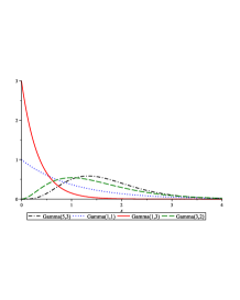
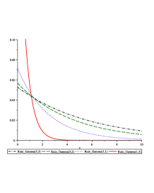
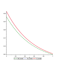
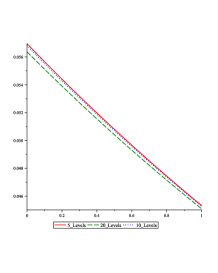
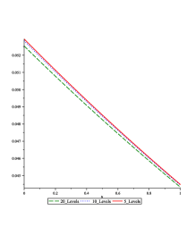
Figure 1: Figures (a) Density function of claim size distributions; (b) to (d) comparison between the ruin probability of such claim size distributions with respect to 5, 10, and 20 premium values scenarios, respectively; (e) to (h) comparison between the ruin probability of 5, 10, and 20 premium values scenarios with respect to different claim size distributions (i.e, Gamma(1,1), Gamma(1,3), Gamma(3,2), Gamma(5,3)).

From the above figures, one may conclude that the ruin probability $\psi(u)$ as function of initial wealth, $u,$ goes to zero and its decay rate depends on tail of its corresponding claim size distribution. Moreover, the ruin probability decreases as the number of premium levels increases. The second observation in different context has been pointed by several authors, see Denuit, et al. (2007) for more detail.

Example 2.

Suppose the claim size is a considerable heavy-tailed distribution with density function

$$f_{X}(x) = 0.150e^{-(x-4)^{2}/2}+\frac{0.075x}{(1+x^{2})^{2}}+0.074e^{-3x}+\frac{0.224e^{-1/(2x)}}{x^{1.5}},x\geq 0$$ (8)

and random premium $C$ has the Gamma distribution with parameters $\kappa=\theta=3.$ Moreover, suppose that the number of sold contracts, $N_{1}(t),$ and number of arrived claims, $N_{2}(t),$ are two independent Poisson processes with intensity $\lambda_{1}=18$ and $\lambda_{2}=11.$ Using a mathematical software such as Maple, one may show that an equation $D(s)=0$ has infinity many simple non-positive roots, see Figure 2(b) for an illustration.

For simplicity, we just considered roots which their both real and imaginary parts are fall within the interval $[-1,2].$ In this subset of complex plane ${\mathbb{C}},$three roots $z_{1}:=-0.5639909305-1.521665917I,$ $z_{2}:=-0.4233614172,$ and $z_{3}:=-0.5639909305+1.521665918I$ have been found. Now using Theorem 2, one may verify that the ruin probability can be evaluated using $\psi(u)=A_{1}e^{z_{1}u}+A_{2}e^{z_{2}u}+A_{3}e^{z_{3}u},$ where

$$A_{1} = -\frac{-M_{1}z_{3}\beta_{23}z_{2}\beta_{32}+M_{1}T_{2}T_{3}+z_{1}\beta_{21}z_{2}\beta_{32}M_{3}+z_{1}\beta_{21}M_{2}T_{3}+z_{1}\beta_{31}T_{2}M_{3}+z_{1}\beta_{31}z_{3}\beta_{23}M_{2}}{T_{1}z_{3}\beta_{23}z_{2}\beta_{32}-T_{1}T_{2}T_{3}+T_{2}z_{3}\beta_{13}z_{1}\beta_{31}+z_{2}\beta_{21}^{2}z_{1}T_{3}+z_{3}\beta_{23}z_{2}\beta_{21}z_{1}\beta_{31}+z_{3}\beta_{13}z_{1}\beta_{21}z_{2}\beta_{32}}$$

$$A_{2} = \frac{-\beta_{21}\beta_{31}M_{3}z_{2}z_{1}-\beta_{21}z_{2}M_{1}T_{3}+\beta_{31}z_{3}\beta_{13}M_{2}z_{1}-z_{2}T_{1}\beta_{32}M_{3}-z_{2}M_{1}z_{3}\beta_{13}\beta_{32}-T_{1}M_{2}T_{3}}{T_{1}z_{3}\beta_{23}z_{2}\beta_{32}-T_{1}T_{2}T_{3}+T_{2}z_{3}\beta_{13}z_{1}\beta_{31}+z_{2}\beta_{21}^{2}z_{1}T_{3}+z_{3}\beta_{23}z_{2}\beta_{21}z_{1}\beta_{31}+z_{3}\beta_{13}z_{1}\beta_{21}z_{2}\beta_{32}}$$

$$A_{3} = \frac{-z_{3}\beta_{23}z_{2}\beta_{21}M_{1}+T_{1}T_{2}M_{3}+T_{1}z_{3}\beta_{23}M_{2}-z_{2}\beta_{21}^{2}z_{1}M_{3}+T_{2}z_{3}\beta_{13}M_{1}+z_{3}\beta_{13}z_{1}\beta_{21}M_{2})}{(T_{1}z_{3}\beta_{23}z_{2}\beta_{32}-T_{1}T_{2}T_{3}+T_{2}z_{3}\beta_{13}z_{1}\beta_{31}+z_{2}\beta_{21}^{2}z_{1}T_{3}+z_{3}\beta_{23}z_{2}\beta_{21}z_{1}\beta_{31}+z_{3}\beta_{13}z_{1}\beta_{21}z_{2}\beta_{32}},$$

where $T_{j}:=\lambda_{2}z_{j}M^{\prime}_{X}(-z_{j})),$ $M_{j}:=\lambda_{2}M_{X}(-z_{j})-\lambda_{2},$ and $\beta_{ij}=(\lambda_{1}+\lambda_{2}-\lambda_{1}M_{C}(z_{i})-\lambda_{2}M_{X}(-z_{j}))/(z_{j}-z_{i})$ for $i,j=1,2,3.$ Therefore, the ruin probability can be approximated by

$$\psi(u_{0}) = \frac{1}{100}||(-0.26+0.52I)e^{(-0.5640-1.5217I)u_{0}}-2.87e^{-0.4234u_{0}}+(-0.26-0.52I)e^{(-0.5640+1.5217I)u_{0}}||.$$

The Cramér-Lundberg upper bound for this situation is $e^{-0.4234u_{0}}$ which is significantly improved by our method, see Figure 2(c).

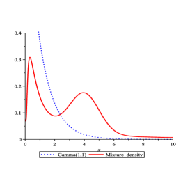
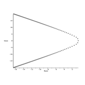
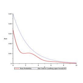
Figure 2: Figures (a) Density function of mixture claim size density 8 accompanied with Gamma (1,1) density function; (b) Roots of equation $D(z)=0$ where $|z|\leq 20\sqrt{2};$ and (c) $\frac{1}{20}\times$ the ruin probability and the Cramér-Lundberg upper bound of the surplus process 1 under mixture claim size density 8.

5 Conclusion and suggestions

The Ruin theory provides some potential tools to study today’s solvency assessments for non-life insurance companies, see Wüthrich (2014) for a practical application. In most practical applications the ruin probability of surplus process 1 has been approximated by the Cramér-Lundberg upper bound $e^{-Ru_{0}},$ where adjustment coefficient $R.$

This article assumed the ruin probability $\psi(\cdot)$ is an exponential type $T$ and $L_{2}({\mathbb{R}})$ function. Then, it derived several approximate formulas for the ruin probability of a double stochastic compound Poisson process. The approximated ruin probability constructed based upon roots of equation $D(s)=0.$ Certainly, $-R$ is one of such roots. Therefore, the Cramér-Lundberg upper bound, multiplied by a constant, will be a part of our approximated ruin probability. Since $-R$ is the largest roots of the equation $D(s)=0,$ our approximation method improved the Cramér-Lundberg upper bound. Such improvement is significant whenever equation $D(s)=0$ has more than one simple non-positive root, see Example 2.

The exponential type assumption can be dropped and a formal solution can be verified by substitution into Equation 4. But, the generally realistic $L_{2}({\mathbb{R}})$ assumption cannot be dropped, because our methods always produce solutions with finite $L_{2}({\mathbb{R}})$ norm. Furthermore, it is essential to our methods that the Laplace transform of $f_{X}$ does not have any branch points in the complex plane.

References

- [1] Ablowitz, M. J. & Fokas, A. S. (1990). Complex variable, introduction and application. Springer-Verlag, Berlin.
- [2] Bao, Z., & Wang, J. (2013). On The Compound Binomial Risk Mondel With Stochastic Income. International Journal of Pure and Applied Mathematics, 82(3), 377-389.
- [3] Bracewell, R. N. (2000). The Fourier transform and its applications. 3rd. ed. McGraw-Hill publisher, New York.
- [4] Cai, J. (2004). Ruin probabilities and penalty functions with stochastic rates of interest. Stochastic process Appl., 112, 53–78.
- [5] Cai, J., & Yang, H. (2014). On the decomposition of the absolute ruin probability in a perturbed compound Poisson surplus process with debit interest. Annals of Operations Research, 212(1), 61–77.
- [6] Champeney, D. C. (1987). A handbook of Fourier theorems. Cambridge University press, New York.
- [7] Denuit, M., Marechal, X., Pitrebois, S., & Walhim, J. F. (2007). Actuarial Modelling of Claim Counts: Risk Classification, Credibility and Bonus–Malus systems. John Wiley & Sons, New York.
- [8] Dym, H. & Mckean, H. P. (1972). Fourier series and integrals. Probability and Mathematical Statistics. Academic Press, New York-London.
- [9] Duffin, R. J. & Schaeffer, A. C. (1937). Some Inequalities concerning functions of Exponential Type. Bull. AMS, 43, 554–556.
- [10] Kaas, R., Goovaerts, M., Dhaene, J., & Denuit, M. (2008). Modern actuarial risk theory: using R.
- [11] Kucerovsky, D. Z. & Payandeh, A. T. (2014). On Ruin Probability Of Long–Term Bonus–Malus Systems. Submitted.
- [12] Gatto, R., & Baumgartner, B. (2014a). Saddlepoint Approximations to the Probability of Ruin in Finite Time for the Compound Poisson Risk Process Perturbed by Diffusion. Methodology and Computing in Applied Probability, (ahead-of-print), 1–19.
- [13] Gatto, R., & Baumgartner, B. (2014b). Value at ruin and tail value at ruin of the compound Poisson process with diffusion and efficient computational methods. Methodology and Computing in Applied Probability, (ahead-of-print), 1–22.
- [14] Landriault, D., & Shi, T. (2014). First passage time for compound Poisson processes with diffusion: ruin theoretical and financial applications. Scandinavian Actuarial Journal, 4, 368–382.
- [15] Lappo, P. M. (2004). Probability of ruin in collective risk model with random premiums. Vestn, Beloruss. Gos. Univ. Ser. 1 Fiz. Mat. Inform, 121, 103–105.
- [16] Lim, S. P. & Qi, L. (2009). A discrete-time risk model with investment and interference under random premium. Applied mathematic: Journal of Chinese university series A., 24, 9–14.
- [17] Melnikov, A. (2011). Risk analysis in finance and insurance. CRC Press.
- [18] Needham, T. (1999). Visual complex analysis. Clarendon press. Oxford.
- [19] Rongming, W., Lin, X., & Dingjun, Y. (2007). Ruin problems with stochastic premium stochastic return on investments. Front. Math. China, 2, 467–490.
- [20] Sasv\a’ri, Z. (2013). Multivariate Characteristic and Correlation Functions.Walter de Gruyter GmbH, Berlin
- [21] Schiff, J. L. (1999). The Laplace transform: Theory and applications. Springer, New York.
- [22] Stein, E. M. (1957). Functions of Exponential Type. Annals of Math, 65, 582–592.
- [23] Temnov, G. (2014). Risk Models with Stochastic Premium and Ruin Probability Estimation. Journal of Mathematical Sciences, 196(1), 84–96.
- [24] Walnut, D. F. (2002). An introduction to wavelet analysis. 2nd ed. Birkhäuser publisher, New York.
- [25] Wüthrich, M. V. (2014). From Ruin Theory To Solvency In Non-life Insurance. Scandinavian Actuarial Journal, (ahead-of-print), 1–11.
- [26] Yu, W. (2013a). Randomized Dividends in a Discrete Insurance Risk Model with Stochastic Premium Income. Mathematical Problems in Engineering, 2013.
- [27] Yu, W. (2013b). On the Expected Discounted Penalty Function for a Markov Regime-Switching Insurance Risk Model with Stochastic Premium Income. Discrete Dynamics in Nature and Society, 2013, 1–9.