Weyl metrics and wormholes

Abstract

We study solutions obtained via applying dualities and complexifications to the vacuum Weyl metrics generated by massive rods and by point masses. Rescaling them and extending to complex parameter values yields axially symmetric vacuum solutions containing singularities along circles that can be viewed as singular matter sources. These solutions have wormhole topology with several asymptotic regions interconnected by throats and their sources can be viewed as thin rings of negative tension encircling the throats. For a particular value of the ring tension the geometry becomes exactly flat although the topology remains non-trivial, so that the rings literally produce holes in flat space. To create a single ring wormhole of one metre radius one needs a negative energy equivalent to the mass of Jupiter. Further duality transformations dress the rings with the scalar field, either conventional or phantom. This gives rise to large classes of static, axially symmetric solutions, presumably including all previously known solutions for a gravity-coupled massless scalar field, as for example the spherically symmetric Bronnikov-Ellis wormholes with phantom scalar. The multi-wormholes contain infinite struts everywhere at the symmetry axes, apart from solutions with locally flat geometry.

1 Introduction

Wormholes are bridges or tunnels between different universes or different parts of the same universe. They were first introduced by Einstein and Rosen (ER) [1], who noticed that the Schwarzschild black hole actually has two exterior regions connected by a bridge. The ER bridge is spacelike and cannot be traversed by classical objects, but it has been argued that it may connect quantum particles to produce quantum entanglement and the Einstein-Pololsky-Rosen (EPR) effect [5], hence ER=EPR [6]. Wormholes were also considered as geometric models of elementary particles – handles of space trapping inside an electric flux, say, which description may indeed be valid at the Planck scale [7]. Wormholes can also describe initial data for the Einstein equations [8] (see [9] for a recent review) whose time evolution corresponds to the black hole collisions of the type observed in the recent GW150914 event [10].

An interesting topic is traversable wormholes – globally static bridges accessible for ordinary classical particles or light [11] (see [12] for a review). In the simplest case such a wormhole is described by a static, spherically symmetric line element

$$ds^{2}=-Q^{2}(r)dt^{2}+dr^{2}+R^{2}(r)(d\vartheta^{2}+\sin^{2}\vartheta d\varphi^{2}),$$ (1.1)

where $Q(r)$ and $R(r)$ are symmetric under $r\to-r$ and $R(r)$ attains a non-zero global minimum at $r=0$. If both $Q$ and $R/r$ approach unity as $r\to\pm\infty$ then the metric describes two asymptotically flat regions connected by a throat of radius $R(0)$. The Einstein equations $G^{\mu}_{\nu}=T^{\mu}_{\nu}$ imply that the energy density $\rho=-T^{0}_{0}$ and the radial pressure $p=T^{r}_{r}$ satisfy at $r=0$

$$\rho+p=-2\frac{R^{\prime\prime}}{R}<0,~{}~{}~{}~{}~{}p=-\frac{1}{R^{2}}<0.$$ (1.2)

It follows that for a static wormhole to be a solution of the Einstein equations, the Null Energy Condition (NEC), $T_{\mu\nu}v^{\mu}v^{\nu}=R_{\mu\nu}v^{\mu}v^{\nu}\geq 0$ for any null $v^{\mu}$, must be violated. Another demonstration [11] of the violation of the NEC uses the Raychaudhuri equation [13] for a bundle of light rays described by $\theta,\sigma,\omega$ : the expansion, shear and vorticity. In the spherically symmetric case one has $\omega=\sigma=0$ [12], hence

$$\frac{d\theta}{d\lambda}=-R_{\mu\nu}v^{\mu}v^{\nu}-\frac{1}{2}\,\theta^{2}\,.$$ (1.3)

If rays pass through a wormhole throat, there is a moment of minimal cross-section area, $\theta=0$ but $d\theta/d\lambda>0$, hence $R_{\mu\nu}v^{\mu}v^{\nu}<0$ and the NEC is violated.

If the spacetime is not spherically symmetric then the above arguments do not apply, but there are more subtle geometric considerations showing that the wormhole throat – a compact two-surface of minimal area – can exist if only the NEC is violated [14, 15]. As a result, traversable wormholes are possible if only the energy density becomes negative, for example due to vacuum polarization [11], or due to exotic matter as for example phantom fields with a negative kinetic energy [16, 17]. Otherwise, one can search for wormholes in the alternative theories of gravity, as for example in the Gauss-Bonnet theory [18], in the brainworld models [19], in theories with non-minimally coupled fields [20], or in massive (bi)gravity [21].

The best known wormhole solutions were found in 1973 in the theory of gravity-coupled phantom scalar field $\psi$ [16, 17]. Their geometry is ultrastatic, $ds^{2}=-dt^{2}+dl^{2}$, where the 3-metric $dl^{2}=\gamma_{ik}dx^{i}dx^{k}$ satisfies equations

$$\overset{(3)}{R}_{ik}(\gamma)=-2\partial_{i}\psi\partial_{k}\psi,~{}~{}~{}~{}~{}~{}~{}~{}\Delta\psi=0,$$ (1.4)

the phantom nature of $\psi$ being encoded in the negative sign in the right hand side of the gravitational equations. The simplest solution of these equations is the spherically symmetric Bronnikov-Ellis (BE) wormhole [16, 17],

$$dl^{2}=dx^{2}+(x^{2}+\mu^{2})(d\vartheta^{2}+\sin^{2}\vartheta d\varphi)^{2},~{}~{}~{}~{}~{}~{}\psi=\arctan\left(\frac{x}{\mu}\right),$$ (1.5)

where $\mu$ is an integration constant determining the size of the wormhole throat. More general solutions of (1.4) were obtained by Clément [22] choosing the 3-metric to be in the axially symmetric Weyl form [23],

$$dl^{2}=e^{2k}(d\rho^{2}+dz^{2})+\rho^{2}d\varphi^{2},$$ (1.6)

where $k$ and $\psi$ depend on $\rho,z$. Equations (1.4) then reduce to

$${\cal D}k=-\rho\left({\cal D}\psi\right)^{2},~{}~{}~{}~{}~{}~{}~{}~{}\frac{1}{\rho}\frac{\partial}{\partial\rho}\left(\rho\,\frac{\partial\psi}{\partial\rho}\right)+\frac{\partial^{2}\psi}{\partial z^{2}}=0,$$ (1.7)

where ${\cal D}=\partial_{\rho}+i\partial_{z}$. Since the $\psi$-equation is linear, superposing its elementary one-wormhole solutions gives solutions describing multi-wormholes [22, 24] (they can be generalized to include also rotation and Maxwell field [25, 26]).

It is worth noting that equations (1.4) actually coincide with the vacuum Einstein equations for the everywhere non-singular 5-metric [27]

$$ds_{5}^{2}=\cos(2\psi)[-dx_{0}^{2}+dx_{4}^{2}]+2\sin(2\psi)dx_{0}dx_{4}+dl^{2}\,.$$ (1.8)

Therefore, wormhole solutions of (1.4) can be interpreted as 5-geometries without invoking the negative energy phantom.

Wormholes are usually associated with exotic matter and it is little known that they exist also in General Relativity (GR) as classical solutions of vacuum Einstein equations. For such solutions the metric is Ricci flat everywhere apart from geometric sets of zero measure that can be interpreted as singular ring-shaped matter sources whose effective energy-momentum tensor has the structure needed to provide the NEC violation. Since these solutions are vacuum everywhere apart from singularities, they can be constructed with the standard GR methods. The first example of this type was discovered in 1966 by Zipoy who studied oblate vacuum metrics of the axially symmetric Weyl type [23] and found solutions which “have a ring singularity and have a double sheeted topology; one can get from one sheet to the other by going through the ring” [29]. The two sheets are the two asymptotically flat regions connected by the wormhole throat – the hole encircled by the ring. As Zipoy noted, this hole should have “strange properties: an object falling through it would not be seen coming out from the other side, whereas if viewed from above the ring it could be seen dropping through” [29]. The ring singularity can be interpreted in this case as a cosmic string loop with the negative tension [30, 31, 32, 33],

$$T=-\frac{(1+\sigma^{2})c^{4}}{4G},$$ (1.9)

where $\sigma$ is a free parameter. Interestingly, if $\sigma=0$ then the metric becomes flat everywhere outside the ring, the latter thus literally creating a hole in flat space [33].

Vacuum ring wormholes may seem to be very different from the BE wormholes supported by the phantom field. However, they are actually described by the same solution. Specifically, the ring metric is

$$ds^{2}=-e^{2U}dt^{2}+e^{-2U}dl^{2}$$ (1.10)

with $dl^{2}$ given by (1.6), and the vacuum Einstein equations read in this case

$${\cal D}k=+\rho\left({\cal D}U\right)^{2},~{}~{}~{}~{}~{}~{}~{}~{}\frac{1}{\rho}\frac{\partial}{\partial\rho}\left(\rho\,\frac{\partial U}{\partial\rho}\right)+\frac{\partial^{2}U}{\partial z^{2}}=0.$$ (1.11)

Now, comparing with (1.7) it is clear that solutions of the two sets of equations are related by

$$U\leftrightarrow\psi,~{}~{}~{}~{}~{}~{}~{}k\leftrightarrow-k.$$ (1.12)

Therefore, ring wormholes and phantom wormholes are actually described by the same equations and to obtain ones from the others it is enough to interchange the phantom $\psi$ with the Newtonian potential $U$ and to flip the sign of $k$. As a result, to study wormholes one can use the ordinary vacuum GR without invoking phantom fields or extra dimensions. The price to pay is the metric singularity supported by the ring which provides the necessary NEC violation.

In this paper we study solutions obtained via applying dualities and complexifications to the vacuum Weyl metrics. As a starting point we use the elementary metrics generated by rods and by point masses. Rescaling them and extending to the complex parameter values yields the prolate and oblate vacuum solutions. Further duality transformations produce a scalar field, which can be either conventional or phantom. This gives rise to large classes of solutions, presumably including all previously known static, axially symmetric solutions for a gravity-coupled massless scalar field. Especially interesting are the oblate solutions which, irrespectively of whether they support a scalar or not, describe wormholes connecting several asymptotic regions. In the one-wormhole sector they reduce to the ring wormholes in the vacuum case, and to the Bronnikov-Ellis wormhole in the phantom case.

The main point we would like to emphasise is that wormholes exist already in vacuum GR. This was known already to Zipoy but remains largely unknown to the community even now. The vacuum wormholes may be viewed as “primary” since those sourced by a scalar can be obtained from them by duality rotations. We shall therefore summarize the essential facts and give a description of the vacuum wormholes, before applying the duality rotations to produce more general solutions with scalar.

The rest of the text is organised as follows. In Section II we introduce the theory of gravitating massless scalar and describe its simplest solutions, both in the case of conventional scalar $\phi$ and for the phantom $\psi$. In Section III we impose the axial symmetry and list the duality transformations which map solutions to solutions. Section IV describes the simplest vacuum Weyl metrics generated by massive rods and by point masses. The vacuum wormholes obtained by rescaling and complexifying the one-rod solution are discussed in Section V, where their topology and the structure of the ring source are considered. This Section also describes solutions with scalar obtained via applying the dualities. Milti-wormholes are considered in Section VI, where we also analyse carefully the regularity at the symmetry axes and describe the two ring and the $N$-ring solutions with locally flat geometry. Finally, we consider in Section VII solutions obtained from the Chazy-Curzon metrics and conclude in Section VIII. The isometric embeddings for the BE wormhole are described in Appendix A, while the relation between work of Famm and that of Einstein-Rosen is discussed in Appendix B.

Unless otherwise stated, Planck units are used everywhere. A short version of this text can be found in [33].

2 Gravitating scalar field

We consider a system with a real gravitating scalar field,

$${\cal L}=[R-2\epsilon\,(\partial\Phi)^{2}]\sqrt{-g}\,.$$ (2.1)

Here the parameter takes two values, either $\epsilon=+1$ corresponding to the conventional scalar field, or $\epsilon=-1$ corresponding to the phantom field. If $\epsilon=+1$ then the energy is positive and the scalar field mediates an attractive force. If $\epsilon=-1$ then the scalar kinetic energy is negative (although the total energy may still be positive) and the corresponding force is repulsive. In what follows we shall be mainly interested in the phantom case, however, it is instructive to consider the two cases together.

Assuming the spacetime metric to be static

$$ds^{2}=-e^{2U}dt^{2}+e^{-2U}\gamma_{ik}dx^{i}dx^{k}$$ (2.2)

where $U$, $\gamma_{ik}$ and $\Phi$ are functions of the spatial coordinates $x^{k}$, the Lagrangian becomes

$${\cal L}=\left[\stackrel{{\scriptstyle(3)}}{{R}}-2\gamma^{ik}(\partial_{i}U\partial_{k}U+\epsilon\,\partial_{i}\Phi\partial_{k}\Phi)\right]\sqrt{\gamma}\,.$$ (2.3)

The field equations are

$$\frac{1}{2}\stackrel{{\scriptstyle(3)}}{{R}}_{ik} = \partial_{i}U\partial_{k}U+\epsilon\,\partial_{i}\Phi\partial_{k}\Phi\,,$$

$$\Delta U = 0\,,$$

$$\Delta\Phi =0\,.$$ (2.4)

In what follows we shall denote $\Phi=\phi$ if $\epsilon=1$ and $\Phi=\psi$ if $\epsilon=-1$. Formally, the change $\epsilon=+1\to\epsilon=-1$ can be achieved by extending the scalar field to purely imaginary values: $\phi\to i\psi$.

Equations (2) admit the following symmetry. If $\epsilon=1$ and $(U,\phi,\gamma_{ik})$ is a solution then the following replacement will give solutions:

$$U \to U\,\cos\alpha+\phi\,\sin\alpha\,,$$

$$\phi \to \phi\,\cos\alpha-U\,\sin\alpha\,,$$

$$\gamma_{ik} \to \gamma_{ik}\,,$$ (2.5)

where $\alpha$ is a constant parameter. Likewise, if $\epsilon=-1$ and $(U,\psi,\gamma_{ik})$ is a solution then other solutions can be obtained via

$${U} \to U\,\cosh\alpha+\psi\,\sinh\alpha\,,$$

$${\psi} \to \psi\,\cosh\alpha+U\,\sinh\alpha\,,$$

$$\gamma_{ik} \to \gamma_{ik}.$$ (2.6)

Many non-trivial solutions can be generated by applying these symmetries, let us consider simple examples.

2.1 Spherically symmetric sector

All known static, spherically symmetric solutions with scalar can be obtained from the vacuum Schwarzschild solution written in the form (here $d\Omega^{2}=d\vartheta^{2}+\sin^{2}\vartheta d\varphi^{2}$)

$$ds^{2} = -\frac{x-m}{x+m}\,dt^{2}+\frac{x+m}{x-m}\,dx^{2}+(x+m)^{2}d\Omega^{2}$$

by applying the rotations (2) or boosts (2). Comparing with the line element (2.2) yields

$$e^{2U}=\frac{x-m}{x+m},~{}~{}~{}~{}~{}~{}~{}\gamma_{ik}dx^{i}dx^{k}=dx^{2}+(x^{2}-m^{2})d\Omega^{2},~{}~{}~{}~{}~{}\Phi=0.$$ (2.7)

2.1.1 Solutions with scalar field $\phi$

Let us choose $\epsilon=+1$, $\Phi=\phi$. Applying to (2.7) the rotation (2) with $\cos\alpha=1/s$ gives

$$e^{2U}=\frac{x-m}{x+m}\to\left(\frac{x-m}{x+m}\right)^{{1}/{s}},~{}~{}~{}~{}~{}~{}~{}~{}e^{2\phi}=1\to\left(\frac{x-m}{x+m}\right)^{{\sqrt{s^{2}-1}}/{s}},$$ (2.8)

while the 3-metric $\gamma_{ik}$ does not change. Therefore,

$$ds^{2} = -\left(\frac{x-m}{x+m}\right)^{{1}/{s}}dt^{2}+\left(\frac{x+m}{x-m}\right)^{{1}/{s}}\left[dx^{2}+(x^{2}-m^{2})d\Omega^{2}\right],$$

$$\phi = \pm\frac{\sqrt{s^{2}-1}}{2s}\ln\left(\frac{x-m}{x+m}\right),~{}~{}~{}~{}~{}~{}~{}~{}~{}|s|\geq 1,$$ (2.9)

which are the well known solutions found by Fisher [35] and by Janis-Robinson-Winicour [36] (FJRW). If $s\to\infty$ then the metric becomes ultra-static,

$$ds^{2}=-dt^{2}+dx^{2}+(x^{2}-m^{2})\,d\Omega^{2},~{}~{}~{}~{}~{}~{}~{}\phi=\pm\frac{1}{2}\ln\left(\frac{x-m}{x+m}\right).$$ (2.10)

2.1.2 Solutions with phantom $\psi$

Let us now set $\epsilon=-1$, $\Phi=\psi$ and apply to (2.7) the boost (2) with $\cosh\alpha=1/s$. This gives the “phantom version” of the FJRW solutions (2.1.1),

$$ds^{2} = -\left(\frac{x-m}{x+m}\right)^{{1}/{s}}dt^{2}+\left(\frac{x+m}{x-m}\right)^{{1}/{s}}\left[dx^{2}+(x^{2}-m^{2})d\Omega^{2}\right],$$

$$\psi = \pm\frac{\sqrt{1-s^{2}}}{2s}\ln\left(\frac{x-m}{x+m}\right)~{}~{}~{}~{}~{}~{}~{}~{}~{}~{}~{}~{}~{}|s|\leq 1.$$ (2.11)

Although the metric looks identical to that in (2.1.1), the geometry is different because the range of $s$ is now different. One may think that these solutions could describe regular black holes, since setting $1/s$ to integer values removes the branching singularity at the horizon $x=m$. However, the area of the sphere is proportional to

$$(x-m)^{1-1/s}\,,$$ (2.12)

hence the horizon has an infinite area, therefore these solutions cannot describe regular black holes.

2.1.3 Wormholes

Let us extend the parameters $m,s$ in (2.1.1), (2.1.2) to imaginary values,

$$m\to i\mu,~{}~{}~{}~{}~{}s\to-is.$$ (2.13)

One has then

$$\frac{x-m}{x+m}\to\frac{x-i\mu}{x+i\mu}=e^{-2i\Psi}\,,~{}~{}~{}~{}~{}~{}\Psi=\arctan\left(\frac{x}{\mu}\right),$$ (2.14)

hence the metric in (2.1.1), (2.1.2) remains real, the scalar field in (2.1.1) becomes purely imaginary, $\phi\to i\psi$, while the phantom field in (2.1.2) remains real, $\psi\to\psi$. As a result, upon the complexification (2.13) both the FJRW solutions (2.1.1) and their phantom counterparts (2.1.2) reduce to the same solutions for the phantom field,

$$ds^{2} = -e^{2\Psi/s}dt^{2}+e^{-2\Psi/s}[dx^{2}+(x^{2}+\mu^{2})d\Omega^{2}]\,,$$

$$\psi = \pm\frac{\sqrt{s^{2}+1}}{s}\,\Psi.$$ (2.15)

These solutions describe globally regular and asymptotically flat wormholes (see the Appendix A where the isometric imbedding of the geometry (2.1.3) into a higher-dimensional Minkowski space is considered). They owe their existence to the repulsive nature of the phantom field – the gravitational attraction being compensated by the scalar field repulsion gives rise to globally regular equilibrium configurations. In the $s\to\infty$ limit one obtains the ultra-static wormhole of Bronnikov and Ellis [16, 17],

$$ds^{2} = -dt^{2}+dx^{2}+(x^{2}+\mu^{2})\,d\Omega^{2}\,,~{}~{}~{}~{}~{}~{}\psi=\pm\Psi.$$ (2.16)

This can also be obtained directly from the ultra-static solution (2.10) via $m\to i\mu$.

2.2 Anti-gravitating solutions with phantom field

Other solutions for the phantom field can be constructed in view of the following observation [38]. Taking the infinite boost limit in (2.1.2),

$$s\to 0,~{}~{}m\to 0,~{}~{}~{}~{}~{}M=-\frac{m}{s}=const,$$ (2.17)

gives

$$ds^{2} = -e^{2U}+e^{-2U}(dx^{2}+x^{2}d\Omega^{2}),~{}~{}~{}~{}~{}~{}U=\frac{M}{x}\,,~{}~{}~{}~{}\psi=\pm U.$$ (2.18)

One notices that the 3-metric $\gamma_{ik}$ becomes flat and $\psi=\pm U$ is a harmonic function. This allows one to generalize the solutions because if $U=\pm\psi$ then Eqs.(2) show that $\stackrel{{\scriptstyle(3)}}{{R}}_{ik}=0$ and hence one can choose $\gamma_{ik}=\delta_{ik}$. The equation for $U$ then becomes $\Delta U=0$ where $\Delta$ is the ordinary Laplace operator. Therefore, any harmonic function $U=\pm\psi$ gives a solution, for example the multi-centre solution,

$$ds^{2} = -e^{2U}+e^{-2U}(d{\bf x})^{2},~{}~{}~{}~{}~{}~{}U=\sum_{n=1}^{N}\,\frac{M_{n}}{|{\bf x}-{\bf x}_{n}|},~{}~{}~{}~{}~{}~{}~{}~{}\psi=\pm U,$$ (2.19)

where $M_{n}$ and ${\bf x}_{n}$ are arbitrary. The existence of such solutions is the speciality of the phantom field whose repulsion can exactly compensate the gravitational attraction.

3 Axially symmetric Weyl metrics and their symmetries

Let us return to equations (2) and assume the system to be axially symmetric. Then the spacetime metric can be put to the Weyl form,

$$ds^{2}=-e^{2U}dt^{2}+e^{-2U}\bigl{\{}e^{2k}\bigl{(}d\rho^{2}+dz^{2}\bigr{)}+\rho^{2}d\varphi^{2}\bigr{\}},$$ (3.1)

where $U,k$ and $\Phi$ depend on $\rho,z$. Then equations (2) reduce to

$$\frac{\partial^{2}U}{\partial\rho^{2}} + \frac{1}{\rho}\,\frac{\partial U}{\partial\rho}+\frac{\partial^{2}U}{\partial z^{2}}=0,$$

$$\frac{\partial^{2}\Phi}{\partial\rho^{2}} + \frac{1}{\rho}\,\frac{\partial\Phi}{\partial\rho}+\frac{\partial^{2}\Phi}{\partial z^{2}}=0,$$

$$\frac{\partial k}{\partial\rho} = \rho\left[\left(\frac{\partial U}{\partial\rho}\right)^{2}-\left(\frac{\partial U}{\partial z}\right)^{2}+\epsilon\left(\frac{\partial\Phi}{\partial\rho}\right)^{2}-\epsilon\left(\frac{\partial\Phi}{\partial z}\right)^{2}\right],$$

$$\frac{\partial k}{\partial z} = 2\rho\,\left[\frac{\partial U}{\partial\rho}\frac{\partial U}{\partial z}+\epsilon\,\frac{\partial\Phi}{\partial\rho}\frac{\partial\Phi}{\partial z}\right].$$ (3.2)

Here the last two equations are compatible with each other in view of the first two equations; their solution can be obtained from the line integral

$$k=\int\left(\frac{\partial k}{\partial\rho}\,d\rho+\frac{\partial k}{\partial z}\,dz\right).$$ (3.3)

This expresses, in principle, $k$ in terms of $U,\Phi$, although in practice the computation of the integral may be difficult. Since $\partial_{z}k\sim\rho$ vanishes at $\rho=0$ (if only $U,\Phi$ are non-singular there), it follows that $k=k_{0}$ at the symmetry axis. If $k_{0}=0$ then the geometry at the axis will be regular, but for $k_{0}\neq 0$ there is a conical singularity on that portion of the axis. Physically this corresponds to a cosmic strut or a cosmic string with deficit angle

$$\delta=2\pi(1-e^{-k_{0}})$$ (3.4)

giving rise to a force or tension

$$T=\frac{\delta}{8\pi}.$$ (3.5)

Such conical singularities are typical for Weyl solutions.

3.1 Symmetries

Equations (3) are invariant under the following operations.

3.1.1 Sign flips and scaling

If $(U,k,\Phi)$ is a solution of Eqs.(3) then the following replacements will give solutions:

$$U\to U,~{}~{}~{}~{} k\to k ,~{}~{}~{}~{}~{}~{}\Phi\to-\Phi;$$

$$U\to-U,~{}~{}~{}~{} k\to k ,~{}~{}~{}~{}\Phi\to\Phi.$$ (3.6)

These symmetries are not very interesting: the first one simply changes sign of the scalar field, while the second one, when applied to solutions (2.1.1),(2.1.2),(2.1.3), changes sign of the parameters $m$ and $\mu$. A more interesting symmetry is

$$U\to\lambda U,~{}~{}~{}~{}k\to\lambda^{2}k,~{}~{}~{}~{}\Phi\to\lambda\Phi,$$ (3.7)

with constant $\lambda$. As we shall see, this symmetry acts in a non-trivial way completely changing properties of solutions.

These three symmetries do not mix up gravitational and scalar variables so that, in particular, vacuum solutions with $\Phi=0$ remain vacuum. There are also symmetries which intermix the variables, they are different for the ordinary scalar field $(\epsilon=+1)$ and for the phantom field $(\epsilon=-1)$.

3.1.2 Rotations and boosts

These symmetries generate solutions with scalar field. The rotations apply only in the conventional scalar case ($\epsilon=+1$ and $\Phi=\phi$) acting on a solution $(U,k,\phi)$ as

$$U\to U\cos\alpha+\phi\sin\alpha,~{}~{}~{}~{}k\to k,~{}~{}~{}~{}\phi\to\phi\cos\alpha-U\sin\alpha,$$ (3.8)

where $\alpha$ is a constant parameter. The boosts apply only in the phantom case ($\epsilon=-1$ and $\Phi=\psi$) acting on $(U,k,\psi)$ as

$$U\to U\cosh\alpha+\psi\sinh\alpha,~{}~{}~{}~{}k\to k,~{}~{}~{}~{}\psi\to\psi\cosh\alpha+U\sinh\alpha.$$ (3.9)

3.1.3 Swap symmetry

This applies only in the phantom field case,

$$U\to\psi,~{}~{}~{}~{}k\to-k,~{}~{}~{}~{}\psi\to U,$$ (3.10)

so that $U$ and $\psi$ swap while $k$ flips sign. The existence of this symmetry implies that there are twice as many solutions with phantom field as those with the ordinary scalar. In particular, this symmetry relates the ring wormholes and the phantom wormholes.

3.1.4 Tachyon symmetry

A complex change of the temporal and azimuthal variables

$$t\to i\varphi,~{}~{}~{}~{}~{}~{}\varphi\to it$$ (3.11)

puts the spacetime metric (3.1) to the form

$$ds^{2}=-\rho^{2}e^{-2U}dt^{2}+e^{-2U}\bigl{\{}e^{2k}\bigl{(}d\rho^{2}+dz^{2}\bigr{)}\bigr{\}}+e^{2U}d\varphi^{2},$$ (3.12)

which is again the Weyl metric obtained from the original one via

$$U\to\ln\rho-U,~{}~{}~{}~{}k\to k-2U+\ln\rho,~{}~{}~{}~{}\Phi\to\Phi.$$ (3.13)

One can check that this is a symmetry of equations (3) which does not change the scalar. This symmetry has been relatively little studied. Applied to the Schwarzschild metric it produces the Peres-Schulman-Gott (PSG) tachyon solution with isometry group $SO(2)\times SO(2,1)$ [39], [40], [41]. This is appropriate for a neutral tachyon moving in a spacetime with one spatial direction compactified; it describes the aftermath of vacuum decay [42].

4 Vacuum Weyl metrics

Let us describe the simplest solutions of Eqs.(3) with $\Phi=0$.

4.1 One-rod solution

The Schwarzschild solution

$$ds^{2}=-e^{2U}dt^{2}+e^{-2U}dl^{2}$$

with

$$e^{2U}=\frac{x-m}{x+m},~{}~{}~{}~{}~{}~{}~{}~{}dl^{2}\equiv\gamma_{ik}dx^{i}dx^{k}=dx^{2}+(x^{2}-m^{2})d\Omega^{2}\,$$ (4.1)

can be transformed to the Weyl form. The transformation is achieved by setting

$$z=x\cos\vartheta,~{}~{}~{}~{}~{}~{}\rho=\sqrt{x^{2}-m^{2}}\sin\vartheta,$$ (4.2)

hence

$$d\rho^{2}+dz^{2}=\frac{x^{2}-m^{2}\cos^{2}\vartheta}{x^{2}-m^{2}}\left[dx^{2}+(x^{2}-m^{2})d\vartheta^{2}\right],$$ (4.3)

which gives

$$ds^{2}=-e^{2U}dt^{2}+e^{-2U}\left[e^{2k}(d\rho^{2}+dz^{2})+\rho^{2}d\varphi^{2}\right],$$ (4.4)

with

$$e^{2U}=\frac{x-m}{x+m},~{}~{}~{}~{}~{}~{}~{}~{}~{}e^{2k}=\frac{x^{2}-m^{2}}{x^{2}-m^{2}\cos^{2}\vartheta}.$$ (4.5)

There remains to express $U,k$ in terms of $\rho,z$. Inverting (4.2) gives $x,\vartheta$ in terms of $z,\rho$,

$$x=R,~{}~{}~{}~{}~{}~{}x\pm m\cos\vartheta=R_{\pm},$$ (4.6)

where

$$R=\frac{1}{2}(R_{+}+R_{-}),~{}~{}~{}~{}~{}~{}~{}~{}~{}R_{\pm}=\sqrt{\rho^{2}+(z\pm m)^{2}}.$$ (4.7)

Injecting this to (4.5) gives $U,k$ expressed in terms of Weyl coordinates,

$$U=\frac{1}{2}\,\ln\left(\frac{R-m}{R+m}\right),~{}~{}~{}~{}~{}~{}~{}~{}~{}~{}~{}k=\frac{1}{2}\ln\left(\frac{R^{2}-m^{2}}{R_{+}R_{-}}\right),$$ (4.8)

and one can directly check that these fulfill equations (3). This gives the Schwarzschild metric in the Weyl form. One notices that $U$ can be represented as the Newtonian potential of a thin rod of linear mass density $1/2$ and of mass $m$, hence

$$U=-\frac{1}{2}\int_{-m}^{m}\frac{d\zeta}{\sqrt{\rho^{2}+(z-\zeta)^{2}}}\,.$$ (4.9)

For this solution one has $k(\rho=0,z)=0$ if $|z|>m$ therefore there are no struts and the geometry is regular on parts of the axis not occupied by the rod.

4.2 Two-rod solution

More general solutions can be obtained by taking several rods and superposing their Newtonian potentials. This gives $U$, while $k$ is obtained from (3.3). In the simplest two-rod case one has [43]

$$U=U_{1}+U_{2},~{}~{}~{}~{}~{}~{}~{}~{}k=k_{1}+k_{2}+k_{12}\,,$$ (4.10)

where (with $a=1,2$)

$$U_{a} = \frac{1}{2}\ln\left(\frac{R_{a}-m_{a}}{R_{a}+m_{a}}\right),~{}~{}~{}~{}~{}~{}~{}~{}k_{a}=\frac{1}{2}\ln\left(\frac{(R_{a})^{2}-(m_{a})^{2}}{R_{a+}R_{a-}}\right),~{}~{}~{}$$

$$k_{12} = \frac{1}{2}\ln\left(\frac{(R_{1+}R_{2-}+z_{1+}z_{2-}+\rho^{2})(R_{1-}R_{2+}+z_{1-}z_{2+}+\rho^{2})}{(R_{1+}R_{2+}+z_{1+}z_{2+}+\rho^{2})(R_{1-}R_{2-}+z_{1-}z_{2-}+\rho^{2})}\right),$$ (4.11)

with

$$z_{a\pm}=z-z_{a}\pm m_{a},~{}~{}~{}~{}~{}~{}~{}~{}R_{a\pm}=\sqrt{\rho^{2}+(z_{a\pm})^{2}}\,,~{}~{}~{}~{}~{}R_{a}=\frac{1}{2}(R_{a+}+R_{a-}).$$ (4.12)

For this solution $k$ vanishes on parts of the $z$-axis non-occupied by the rods, except for the interval between the rods where it is constant and negative. Therefore, there is a negative tension strut between the two rods giving rise to the repulsive force. This strut “props up” the two black holes and does not let them fall on each other.

The generalization to $N$ rods is straightforward [43],

$$U=\sum_{a=1}^{N}U_{a},~{}~{}~{}~{}~{}~{}~{}~{}k=\sum_{a=1}^{N}k_{a}+\sum_{a<b}k_{ab}\,,$$ (4.13)

where $U_{a},k_{a}$ are given by the same expressions as in (4.2), while $k_{ab}$ is obtained from $k_{12}$ in (4.2) by replacing $R_{1\pm}\to R_{a\pm}$ and $R_{2\pm}\to R_{b\pm}$.

4.3 The Chazy-Curzon metrics

Instead of the Newtonian potential of rods one can consider that of point masses located at the $\rho=0$ axis. For just one mass $m$ located at $z=0$ one obtains the solution

$$U=-\frac{m}{R}\,,\qquad k=-\frac{m^{2}\rho^{2}}{2R^{4}}\,,$$ (4.14)

where $R=\sqrt{\rho^{2}+z^{2}}$.

For two masses $m_{\pm}$ located $z=\pm m$ one has, with $R_{\pm}=\sqrt{\rho^{2}+(z\pm m)^{2}}$,

$$U = -\frac{m_{+}}{R_{+}}-\frac{m_{-}}{R_{-}},$$

$$k = -\frac{m_{+}^{2}\rho^{2}}{2(R_{+})^{4}}-\frac{m_{-}^{2}\rho^{2}}{2(R_{-})^{4}}+\frac{m_{+}m_{-}}{2m^{2}}\left(\frac{\rho^{2}+z^{2}-m^{2}}{R_{+}R_{-}}-1\right).$$ (4.15)

These solutions were constructed by Chazy [44] and Curzon [45] and later independently by Silberstein [46]. The one-mass solution is regular at the axis, while for the two masses one has

$$k(\rho=0,z)=\frac{m_{+}m_{-}}{2m^{2}}\left(\frac{z^{2}-m^{2}}{|z^{2}-m^{2}|}-1\right).$$ (4.16)

This vanishes outside the interval between the two particles where $z^{2}-m^{2}>0$ but not inside this interval where $z^{2}-m^{2}<0$ and hence [47]

$$k(\rho=0,z)=-\frac{m_{+}m_{-}}{m^{2}}.$$ (4.17)

The original paper of Curzon [45] also gives the solution for $N$ point masses.

5 Solutions from one rod

We described above the elementary vacuum solutions generated by rods and by point masses. One could now apply rotations (3.8) and boosts (3.9) to produce new solutions with scalar field. However, before doing this we notice that yet much larger families of vacuum metrics can be obtained via acting first with the scale symmetry (3.7) and then performing complexification. This gives the prolate and oblate vacuum metrics.

5.1 Prolate vacuum metrics

Applying the scaling (3.7) to the one-rod Schwarzschild solution (4.8) gives the two-parameter family of solutions labeled by $\lambda$ and $m$,

$$U=\frac{\lambda}{2}\,\ln\left(\frac{R-m}{R+m}\right),~{}~{}~{}~{}~{}~{}~{}~{}~{}~{}~{}k=\frac{\lambda^{2}}{2}\ln\left(\frac{R^{2}-m^{2}}{R_{+}R_{-}}\right),$$ (5.1)

with

$$R=\frac{1}{2}(R_{+}+R_{-}),~{}~{}~{}~{}R_{\pm}=\sqrt{\rho^{2}+(z\pm m)^{2}}.$$ (5.2)

Using (4.2), (4.3), (4.5) to pass back to the $x,\vartheta$ coordinates gives

$$ds^{2} = -\left(\frac{x-m}{x+m}\right)^{\lambda}dt^{2}+\left(\frac{x-m}{x+m}\right)^{-\lambda}dl^{2},$$ (5.3)

$$dl^{2} = \left(\frac{x^{2}-m^{2}\cos^{2}\vartheta}{x^{2}-m^{2}}\right)^{1-\lambda^{2}}\left[dx^{2}+(x^{2}-m^{2})d\vartheta^{2}\right]+(x^{2}-m^{2})\sin^{2}\vartheta d\varphi^{2}\,.$$

These are the prolate Zipoy-Voorhees (ZV) solutions [29, 50]. Unless for $\lambda^{2}=1$ they are not spherically symmetric and exhibit a curvature singularity at $R=x=m$. These metrics have been relatively well studied, as they can be used to describe deformations of the Schwarzschild black hole (see for example [51, 52]). For all these solutions the relation between the $x,\vartheta$ and $\rho,z$ coordinates is given by (4.2), hence

$$\frac{z^{2}}{x^{2}}+\frac{\rho^{2}}{x^{2}-m^{2}}=1.$$ (5.4)

Therefore, lines of constant $x$ are prolate ellipses with the major semi-axis oriented along the $z$-direction. In the $x\to m$ limit these ellipses shrink to the $-m\leq z\leq m$ segment of the $z$-axis. Both $(\rho,z)$ and $(x,\vartheta)$ coordinate cover the $R=x>m$ region of the manifold.

5.2 Oblate vacuum metrics

Let us continue the solution (5.1) to imaginary parameter values,

$$m\to i\mu\,,~{}~{}~{}~{}~{}~{}~{}~{}~{}~{}~{}\lambda\to i\sigma.$$ (5.5)

In this case instead of (4.2) one will have

$$z=x\cos\vartheta,~{}~{}~{}~{}~{}~{}\rho=\sqrt{x^{2}+\mu^{2}}\,\sin\vartheta,$$ (5.6)

hence

$$\frac{z^{2}}{x^{2}}+\frac{\rho^{2}}{x^{2}+\mu^{2}}=1.$$ (5.7)

Therefore, lines of constant $x$ in the $(\rho,z)$ plane are oblate ellipses with the major semi-axis oriented along the $\rho$-direction. In the $x\to 0$ limit these ellipses shrink to the segment of the $\rho$-axis

$${\cal I}=\{\rho\in[0,\mu],z=0\}$$ (5.8)

(assuming that $\mu>0$). The functions $R_{\pm}$ in (5.2) become complex-valued,

$$R_{\pm}=\sqrt{\rho^{2}+(z\pm m)^{2}}~{}~{}\to~{}~{}\sqrt{\rho^{2}+(z\pm i\mu)^{2}}\equiv X\pm iY,$$ (5.9)

with

$$X=\pm{\cal X},~{}~{}~{}~{}~{}Y=\pm{\rm sign}(z)\,{\cal Y},$$ (5.10)

where

$${\cal X}=\frac{1}{\sqrt{2}}\sqrt{\sqrt{A^{2}+B^{2}}+A}\,,~{}~{}~{}~{}~{}~{}~{}~{}~{}~{}~{}~{}~{}{\cal Y}=\frac{1}{\sqrt{2}}\sqrt{\sqrt{A^{2}+B^{2}}-A}\,,$$ (5.11)

with $A=\rho^{2}+z^{2}-\mu^{2}$ and $B=2\mu z$. Since $R$ is replaced by a real quantity,

$$R=\frac{1}{2}(R_{+}+R_{-})\to X,$$ (5.12)

and one has

$$\frac{1}{2}\ln\left(\frac{R-m}{R+m}\right)\to\frac{1}{2}\ln\left(\frac{X-i\mu}{X+i\mu}\right)=-i\arctan\left(\frac{X}{\mu}\right),$$ (5.13)

it follows that the solution remains real-valued,

$$U=\sigma\arctan\left(\frac{X}{\mu}\right),~{}~{}~{}~{}~{}~{}~{}~{}~{}k=\frac{\sigma^{2}}{2}\ln\left(\frac{X^{2}+Y^{2}}{X^{2}+\mu^{2}}\right).$$ (5.14)

These are the oblate Zipoy-Voorhees solutions [29, 50]. These solutions are relatively little known, therefore we shall describe some of their properties.

The two sign choices $``\pm"$ in (5.10) correspond to the two square root branches. For each branch the real and imaginary parts of the square root, $X$ and $Y$, are discontinuous and/or not smooth at the branch cut along the segment (5.8). However, gluing the two branch sheets together gives a Riemann surface on which all functions are smooth and continuous. The functions $X$, $Y$ defined by (5.10) are already smooth and continuous for $\rho>\mu$, while for $\rho<\mu$ one should analytically continue them through the cut, which is achieved by replacing

$$X\to{\rm sign}(z)X=\pm{\rm sign}(z){\cal X},~{}~{}~{}~{}~{}~{}Y\to{\rm sign}(z)Y=\pm{\cal Y}.$$ (5.15)

These functions are continuous for $\rho<\mu$ (although discontinuous for $\rho>\mu$). In particular, at the symmetry axis one has after the analytic continuation either $X=z$, $Y=\mu$ or $X=-z$, $Y=-\mu$.

   

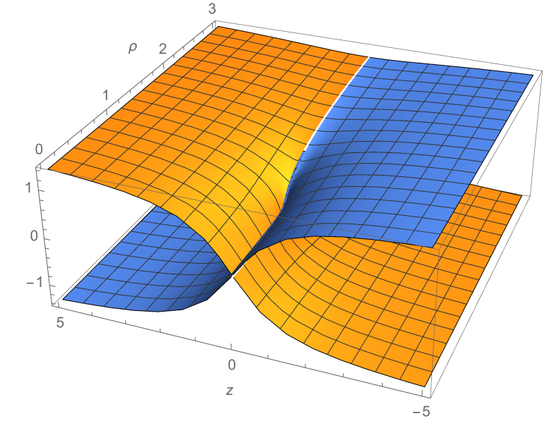
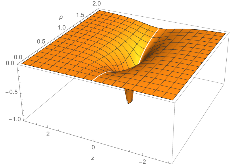
Figure 1: $U(\rho,z)$ (left) and $k(\rho,z)$ (right) for the solution (5.14) with $\sigma=\mu=1$. The two branches of $U$ (blue and yellow online) correspond to $X$ chosen according (5.15).

As a result, one obtains the plots of the solution (5.14) shown in Fig.1. The function $U(\rho,z)$ is double-valued while $k(\rho,z)$ is single-valued and vanishes at the symmetry axis. The two different values of $U$ for given $\rho,z$ correspond to two different spacetime points.

5.2.1 Wormhole topology

As first noticed by Zipoy [29], solutions (5.14) describe wormholes. This can be seen by making the complexification (5.5) directly in (5.3), which gives

$$ds^{2} = -e^{2U}dt^{2}+e^{-2U}dl^{2},~{}~{}~{}~{}~{}~{}~{}~{}~{}~{}~{}~{}~{}U=\sigma\arctan\left(\frac{x}{\mu}\right),$$ (5.16)

$$dl^{2} = \left(\frac{x^{2}+\mu^{2}\cos^{2}\vartheta}{x^{2}+\mu^{2}}\right)^{1+\sigma^{2}}\left[dx^{2}+(x^{2}+\mu^{2})d\vartheta^{2}\right]+(x^{2}+\mu^{2})\sin^{2}\vartheta d\varphi^{2}\,.$$

This is the standard form of the oblate Zipoy-Voorhees solutions [29, 50]. When written in this form, it is seen that these metrics describe wormholes with two asymptotically flat for $x\to\pm\infty$ regions connected by a throat at $x=0$. This is obvious already by noticing that close to the symmetry axis where $\cos^{2}\vartheta\approx 1$ the metric (5.16) reduces to the wormhole metric (2.1.3) (up to the replacement $\sigma\to 1/s$).

The coordinates $(x,\vartheta)$ are global and all their functions are single-valued, while the Weyl coordinates are not global and one needs two Weyl charts [22]

$$D_{\pm}:\{\rho\geq 0,\,-\infty<z<\infty\}$$ (5.17)

to cover the manifold. Let us discuss the relation between the two coordinate systems.

The $(\rho,z)$ coordinates are related to $(x,\vartheta)$ via (5.6),

$$z=x\cos\vartheta,~{}~{}~{}~{}\rho=\sqrt{x^{2}+\mu^{2}}\,\sin\vartheta,$$ (5.18)

therefore,

$$X\pm iY=\sqrt{\rho^{2}+(z\pm i\mu)^{2}}=\sqrt{(x\pm i\mu\cos\vartheta)^{2}}=x\pm i\mu\cos\vartheta,$$ (5.19)

hence

$$x=X(\rho,z),~{}~{}~{}~{}~{}~{}\mu\cos\vartheta=Y(\rho,z),$$ (5.20)

which gives inverse transformation from $(\rho,z)$ to $(x,\vartheta)$. Since for given $(\rho,z)$ there are two different branches of $(X,Y)$ defined by (5.10), the inverse transformation is double-valued – the same pair of values $(\rho,z)$ can correspond either to $(x,\vartheta)$ or to $(-x,\pi-\vartheta)$. Therefore, the $D_{+}$ chart covers the “positive” ($x>0$) wormhole side while the $D_{-}$ chart covers the “negative” ($x<0$) side (see Fig.2) [53].

   

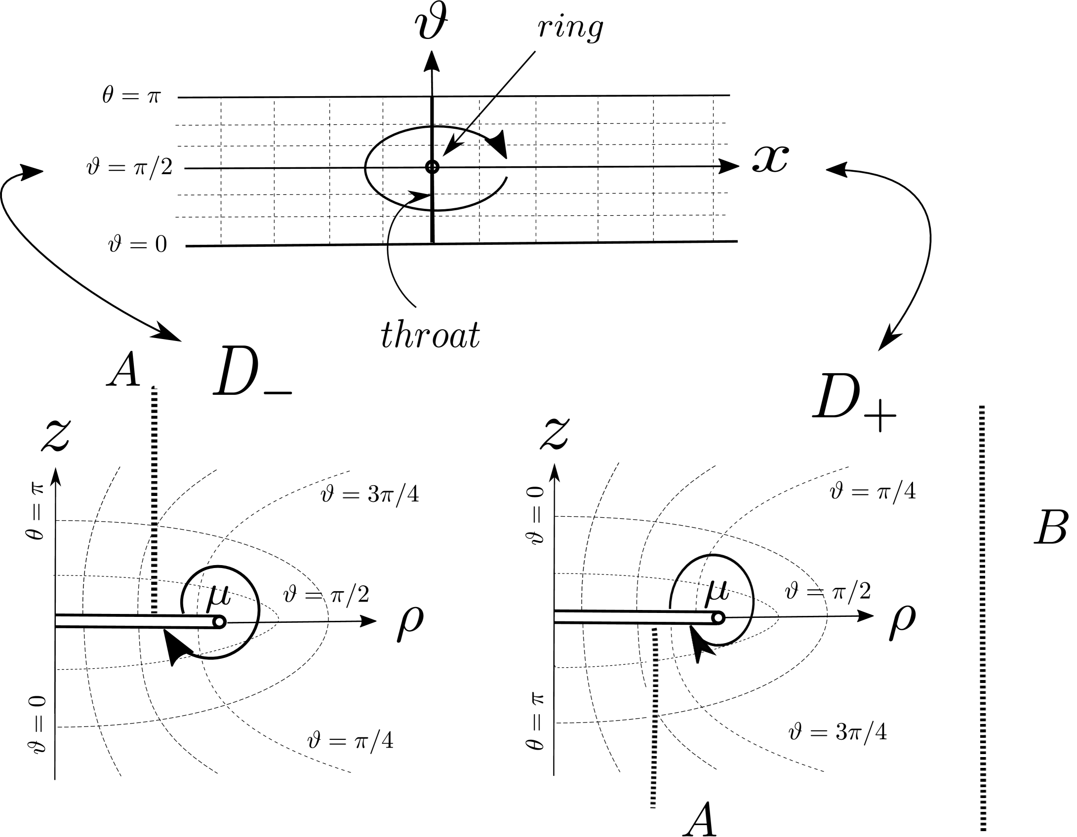
Figure 2: Wormhole topology: The $x,\vartheta$ coordinates cover the whole of the manifold, while each of the two Weyl charts $D_{+}$ and $D_{-}$ covers only either the $x>0$ or $x<0$ part of the manifold. The upper edge of the cut in the $D_{+}$ patch is identified with the lower edge of the $D_{-}$ cut and vice-versa. A winding around the ring in the $x,\vartheta$ coordinates corresponds to two windings in Weyl coordinates.

The symmetry axis in Weyl coordinates, $\rho=0$, $z\in(-\infty,+\infty)$, has two images in the spacetime: either $\vartheta=0$, $z=x$ or $\vartheta=\pi$, $z=-x$. Therefore, the spacetime actually has two symmetry axes, one at $\vartheta=0$ and one at $\vartheta=\pi$, corresponding to the edges of the $(x,\vartheta)$ strip in Fig.2. This explains, in particular, the two values of $U(\rho,z)$ in Fig.1. For example, at $\rho=0$ one has for the (yellow online in Fig.1) branch of $U(\rho,z)$ with $X=x=z$ and $Y=\mu$

$$U(0,z)=\sigma\arctan\left(\frac{z}{\mu}\right)=\sigma\arctan\left(\frac{x}{\mu}\right).$$ (5.21)

This gives the value at the $\vartheta=0$ axis. Similarly, for the second (blue online) branch of $U$ in Fig.1 one has $X=x=-z$ and $Y=-\mu$ at $\rho=0$, hence

$$U(0,z)=-\sigma\arctan\left(\frac{z}{\mu}\right)=\sigma\arctan\left(\frac{x}{\mu}\right),$$ (5.22)

which gives the value at the $\vartheta=\pi$ axis. These two values of $U(0,z)$ coincide when expressed in terms of the $x$-coordinate.

It is also instructive to pass to the Weyl coordinates directly in (5.16). The starting point is the line element

$$dl^{2} = dx^{2}+(x^{2}+\mu^{2})(d\vartheta^{2}+\sin^{2}\vartheta d\varphi^{2})$$ (5.23)

where $x\in(-\infty,\infty)$. This can be transformed to the isotropic form by setting

$$x=\frac{\chi^{2}-\mu^{2}}{2\chi}~{}~{}~{}~{}\Leftrightarrow~{}~{}~{}~{}\chi=x+\sqrt{x^{2}+\mu^{2}}\in[0,\infty),$$ (5.24)

which gives

$$dl^{2}=\frac{1}{4}\left(1+\frac{\mu^{2}}{\chi^{2}}\right)^{2}[d\chi^{2}+\chi^{2}d\vartheta^{2}+\chi^{2}\sin^{2}\vartheta d\varphi^{2}].$$ (5.25)

Introducing the complex variable

$$\omega=i\chi e^{-i\vartheta}=\chi\sin\vartheta+i\chi\cos\vartheta$$ (5.26)

one obtains

$$dl^{2}=\frac{1}{4}\left(1+\frac{\mu^{2}}{|\omega|^{2}}\right)^{2}[|d\omega|^{2}+(\Re(\omega))^{2}d\varphi^{2}].$$ (5.27)

The $\omega$-variable sweeps the upper half-plane $\Re(\omega)\geq 0$ such that the $x<0$ and $x>0$ regions map, respectively, to the $|\omega|<\mu$ and $|\omega|>\mu$ regions. Passing to the new complex variable $\omega\to w(\omega)$ via the Joukowski transformation [25],

$$w=\frac{1}{2}\left(\omega+\frac{\mu^{2}}{\omega}\right)\equiv\rho+iz,$$ (5.28)

one finds that $\rho=\Re(w)$ and $z=\Im(w)$ are related to $x,\vartheta$ by (5.18), whereas the metric becomes

$$dl^{2} = \frac{1}{4}\left(1+\frac{\mu^{2}}{|\omega|^{2}}\right)^{2}\left|\frac{d\omega}{dw}\right|^{2}|dw|^{2}+\rho^{2}d\varphi^{2}.$$ (5.29)

As a result, one has

$$dx^{2}+(x^{2}+\mu^{2})d\vartheta^{2} = \frac{1}{4}\left(1+\frac{\mu^{2}}{|\omega|^{2}}\right)^{2}\left|\frac{d\omega}{dw}\right|^{2}|dw|^{2}=\frac{x^{2}+\mu^{2}}{x^{2}+\mu^{2}\cos^{2}\vartheta}(dz^{2}+d\rho^{2}),$$

$$(x^{2}+\mu^{2})\sin^{2}\vartheta d\varphi^{2} = \rho^{2}d\varphi^{2},$$ (5.30)

using which and assuming (5.20), the solution (5.16) takes up the Weyl form with $U,k$ given by (5.14).

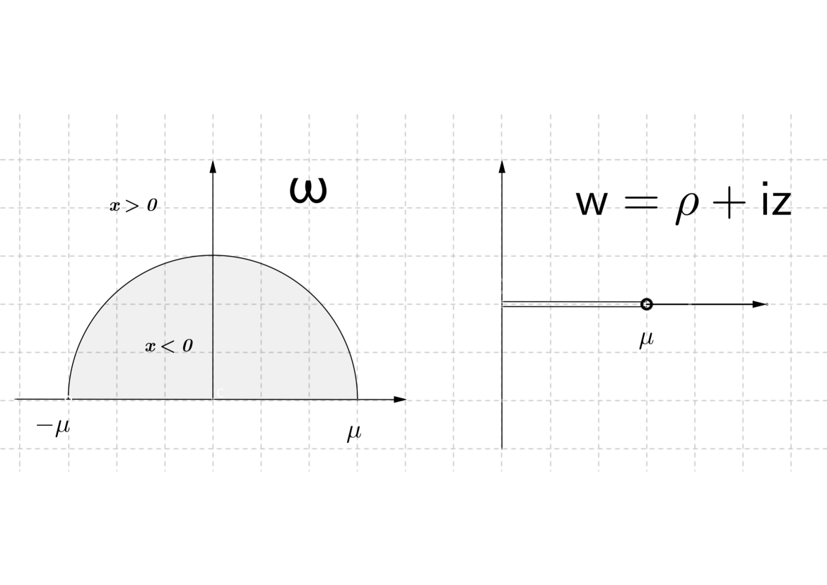
Figure 3: The Joukowski function (5.28) maps the interior $(x<0)$ of the semi-cercle $|\omega|=\mu$, $\Im(\omega)\geq 0$ to a half-plane $\Re(w)\geq 0$ with a cut removed, which corresponds to the $D^{-}$ Weyl region. The exterior $(x>0)$ of the semi-circle maps similarly to the $D^{+}$ Weyl region.

The Joukowski transformation $\omega\to w$ (5.28) maps the regions $|\omega|<\mu$ and $|\omega|>\mu$ of the $\omega$-plane to the whole $w$-plane with the removed segment or real axis,

$$w\in[-\mu,\mu].$$ (5.31)

The inverse Joukowski transformation

$$\omega=w\pm\sqrt{w^{2}-\mu^{2}}$$ (5.32)

has branching points at $w=\pm\mu$ connected by the branch cut (5.31). Any closed contour intersecting the cut passes from one Riemann sheet to the other and the sign of the square root in (5.32) changes. As a result, the full Riemann surface on which the Joukowski function is single-valued consistes of two sheets glued together through the cut (5.31).

Restricting now to the upper half-plane $\Im(\omega)\geq 0$, the “positive” ($|\omega|>\mu$) and “negative” ($|\omega|<\mu$) wormhole sides map, respectively, to the $D_{+}$ and $D_{-}$ Weyl regions (5.17), each region having the branch cut (5.8) removed (see Fig.3). The entire coordinate atlas of the spacetime manifold is obtained by identifying the upper edge of the cut on the $D_{+}$ chart with the lower edge of the cut on the $D_{-}$ chart and vice-versa. The negative part of the $z$-axis in the $D_{-}$ patch then merges with the positive part of the $z$-axis in the $D_{+}$ patch (see Fig.2), which gives the $\vartheta=0$ axis; similarly for the $\vartheta=\pi$ axis.

It is worth emphasising again that the wormhole features of the oblate vacuum solutions had been recognised already in 1966 by Zipoy [29], but even now these solutions remain very little known.

5.2.2 Ring wormholes

The branching point of the Weyl coordinates at $\rho+iz=\mu$ gives rise to a curvature singularity at $x=0$, $\vartheta=\pi/2$, that is along a circle of radius $\mu$ placed in the equatorial plane. The curvature consists of the Ricci part and of the Weyl part, which show, respectively, a distributional singularity and a power-law singularity. Consider first the distributional part. This arises because the Ricci tensor vanishes everywhere (the metric is vacuum) apart form the ring where it shows a delta-type singularity.

Setting $x=\mu\,x_{1}$ and $\cos\vartheta=x_{2}$, the metric (5.16) becomes

$$ds^{2} = -e^{2U}dt^{2}+e^{-2U}dl^{2},~{}~{}~{}~{}~{}~{}~{}~{}~{}~{}~{}~{}~{}U=\sigma\arctan\left(x_{1}\right),$$ (5.33)

$$dl^{2} = \mu^{2}\left(\frac{x_{1}^{2}+x_{2}^{2}}{x_{1}^{2}+1}\right)^{1+\sigma^{2}}\left[dx_{1}^{2}+\frac{x_{1}^{2}+1}{1-x_{2}^{2}}\,dx_{2}^{2}\right]+\mu^{2}(x_{1}^{2}+1)(1-x_{2}^{2})\,d\varphi^{2}\,.$$

Expanding this for small $x_{1},x_{2}$ yields in the leading order

$$ds^{2}=-dt^{2}+\mu^{2}\left({x_{1}^{2}+x_{2}^{2}}\right)^{1+\sigma^{2}}(dx_{1}^{2}+dx_{2}^{2})+\mu^{2}d\varphi^{2}+\ldots,$$ (5.34)

where the dots denote the subleading terms. Passing to polar coordinates $r,\theta$ via

$$(x_{1}+ix_{2})^{q}=\frac{q}{\mu}\,{r}e^{i\theta}$$ (5.35)

with $q=2+\sigma^{2}$ yields

$$ds^{2}=-dt^{2}+dr^{2}+r^{2}d\theta^{2}+\mu^{2}d\varphi^{2}+\ldots$$ (5.36)

This metric looks flat, but since the angular variable $\theta$ ranges from zero to $2\pi q>2\pi$ after a revolution around the point $r=0$, there is a negative angle deficit,

$$\delta=2\pi-2\pi q=-(\sigma^{2}+1)2\pi,$$ (5.37)

which gives rise to a conical singularity of the Ricci tensor $r=0$. This can be associated to a distributional matter source – an infinitely thin ring of radius $\mu$ and of negative tension (energy per unit length) [33]

$$T=-\frac{(1+\sigma^{2})c^{4}}{4G}$$ (5.38)

(the correct physical dimensions are restored here for the moment). The ring encircles the wormhole throat and plays the role of the negative energy source for the solution.

Consider now the power-law singularity of the Riemann tensor. Although the leading terms of the line element in (5.36) describe a (locally) flat geometry, the subleading terms denoted by the dots produce a non-zero curvature. Since these terms vanish for $x_{1},x_{2}\to 0$, one could expect the curvature to vanish in this limit too. Surprisingly, just the opposite happens and the curvature diverges for $x_{1},x_{2}\to 0$ because the subleading terms do not vanish fast enough in this limit. To understand this, consider just one metric component,

$$g_{\varphi\varphi}=\mu^{2}\exp[-2\sigma\arctan(x_{1})](x_{1}^{2}+1)(1-x_{2}^{2})=\mu^{2}(1+\ldots).$$ (5.39)

Keeping only the leading order term here would give a constant, $\mu^{2}$, whose derivatives vanish and give no contribution to the curvature. However, keeping also the subleading terms, the second derivatives $\partial_{11}g_{\varphi\varphi}$ and $\partial_{22}g_{\varphi\varphi}$ and the $R_{1\varphi 1\varphi}$ and $R_{2\varphi 2\varphi}$ curvature components do not vanish at $x_{1},x_{2}\to 0$, implying that the curvature invariant diverges. A direct computation yields

$$R_{\mu\nu\alpha\beta}R^{\mu\nu\alpha\beta}=\frac{\sigma^{2}}{\mu^{4}}\frac{16(1+\sigma^{2})^{2}}{(x_{1}^{2}+x_{2}^{2})^{3+2\sigma^{2}}}\,(1+\ldots)$$ (5.40)

(the dots denoting terms that vanish for $x_{1},x_{2}\to 0$) hence the curvature is unbounded for small $x_{1},x_{2}$. This shows that the form of the line element (5.36) is somewhat deceptive – even though close to the ring it manifestly approaches flat metric (with an angle deficit), the curvature grows.

Summarising, the ring carries the distributional conical singularity and also the power-law singularity of the curvature.

Notice that the curvature tends to zero if $\mu\to\infty$. This is natural, since in this limit the ring radius tends to infinity. Each its finite segment then approaches a piece of an infinite straight cosmic string whose geometry is locally flat. Therefore, one can view the Weyl curvature of the ring as an effect of bending the cosmic string.

Another remarkable limit where the geometry becomes locally flat is obtained by taking $\sigma\to 0$. The curvature then vanishes since the functions $U,k$ in (5.14) vanish and the metric expressed in Weyl coordinates becomes manifestly flat,

$$ds^{2}=-dt^{2}+d\rho^{2}+dz^{2}+\rho^{2}d\varphi^{2}.$$ (5.41)

However, the topology is still non-trivial because the $(\rho,z)$ coordinates do not cover the whole of the manifold but only either the $D_{+}$ or $D_{-}$ patches glued to each other through the cuts. A contour around the ring core in the $D_{+}$ patch does not close after a revolution of $2\pi$ but passes to the $D_{-}$ patch and only after a second revolution of $2\pi$ returns back to the initial position (see Fig.2). Therefore, the winding angle around the ring core ranges from zero to $4\pi$, which indicates that the ring is still there and has the tension

$$T=-\frac{c^{4}}{4G}.$$ (5.42)

As a result, the ring supports only the conical singularity while the geometry is locally exactly flat.

It follows that the geodesics which do not hit the ring are simply straight lines as in flat space. Those which pass outside the ring always stay in the same coordinate chart (line B in Fig.2), while those threading the ring pass to the other chart and become invisible from the previous chart thus traversing the wormhole (line A in Fig.2). Therefore, the ring genuinely cuts a hole in flat space through which on can observe another universe and get there. This reminds one of Alice observing the room behind the looking glass and next jumping there. An object falling through the ring can be seen from behind, while viewed from the side it is not seen coming from the other side (see Fig.4).

   

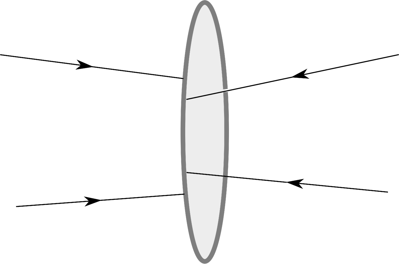
Figure 4: Particles entering the ring are not seen coming out from the other side

It seems plausible that the wormhole edges could be smoothened without changing the global structure if the singular ring is replaced by a regular hoop-shaped energy distribution of finite thickness and with the same tension. Inside the hoop the energy density is finite hence the geometry must be regular, while outside the energy is zero and the geometry should be more or less the same as for the original ring. This suggests that wormholes could be created by negative energies concentrated in toroidal volumes, for example by vacuum fluctuations. Therefore, traversable wormholes could actually be more than just a mathematical curiosity.

However, the energy needed to create a ring wormhole is very high. The absolute value of the negative tension $T$ in (5.42) coincides with the highest possible value for a positive tension (force), according to the maximum tension principle in General Relativity conjectured in [54, 55]. This conjecture is supported, for example, by the fact that the angle deficit of a cosmic string cannot exceed $2\pi$. Numerically one has ${T}=-3.0257\times 10^{43}$ Newtons $\approx-3\times 10^{39}$ Tonnes, hence to create a macroscopic ring wormhole of radius $R=1$ metre, say, one needs a negative energy equivalent to the mass of Jupiter, $2\pi RT/c^{2}\approx 10^{-3}M_{\odot}$ [33, 56].

At the same time, one can also imagine microscopically small rings by quantum fluctuations appearing spontaneously from the vacuum and then disappearing again. Particles crossing the ring during its existence would no longer be accessible from our universe after the ring disappears. If true, this would be a potential mechanism for the loss of quantum coherence.

It is worth noting that the $\sigma=0$ ring wormhole with locally flat geometry can be viewed as a particular case of the so called “star gate wormholes” constructed by surgeries and identifications performed on Minkowski space [12]. In such a construction two copies of Minkowski space are identified over a boundary of a compact 3-region removed from each copy and the geometric junction conditions determine the surface energy density, which is negative for convex surfaces. In the simplest cases such wormholes are “cubic” or “polyhedral” with the negative energy localized only along the polyhedra edges [57]. Their particular limit are planar “dihedral wormholes”, which in their turn reduce to “loop based wormholes” when the number of edges tends to infinity [12]. For such wormholes the negative energy is distributed along a loop of arbitrary shape encircling the wormhole throat, the geometry being exactly flat outside the loop. Remarkably, the loop tension turns out to be precisely the same as the value (5.42) obtained in our analysis by completely different methods. As a result, our estimate of the negative energy equivalent to the mass of Jupiter needed to create a one meter size wormhole is actually the same as the one previously quoted in the literature [12].

5.3 Solutions with scalar field

We can now produce new solutions with scalar field by applying the rotations (3.8) and boosts (3.9) to the prolate and oblate vacuum metrics written in the form (5.3) and (5.16). Applying the rotation (3.8) produces solutions with the conventional scalar in the prolate case,

$$ds^{2} = -\left(\frac{x-m}{x+m}\right)^{\lambda/s}dt^{2}+\left(\frac{x-m}{x+m}\right)^{-\lambda/s}dl^{2},~{}~{}~{}~{}\phi=\frac{\sqrt{s^{2}-1}}{s}\,\frac{\lambda}{2}\ln\left(\frac{x-m}{x+m}\right),$$

$$dl^{2} = \left(\frac{x^{2}-m^{2}\cos^{2}\vartheta}{x^{2}-m^{2}}\right)^{1-\lambda^{2}}\left[dx^{2}+(x^{2}-m^{2})d\vartheta^{2}\right]+(x^{2}-m^{2})\sin^{2}\vartheta d\varphi^{2},$$ (5.43)

and in the oblate case,

$$ds^{2} = -e^{2(\sigma/s)\Psi}dt^{2}+e^{-2(\sigma/s)\Psi}dl^{2},~{}~{}~{}~{}~{}\phi=\sigma\frac{\sqrt{s^{2}-1}}{s}\,\Psi,$$ (5.44)

$$dl^{2} = \left(\frac{x^{2}+\mu^{2}\cos^{2}\vartheta}{x^{2}+\mu^{2}}\right)^{1+\sigma^{2}}\left[dx^{2}+(x^{2}+\mu^{2})d\vartheta^{2}\right]+(x^{2}+\mu^{2})\sin^{2}\vartheta d\varphi^{2},$$

where $\Psi=\arctan(x/\mu)$ and $s\geq 1$. Applying boosts (3.9) gives solutions with the phantom field – boosted prolate solutions,

$$ds^{2} = -\left(\frac{x-m}{x+m}\right)^{\lambda/s}dt^{2}+\left(\frac{x-m}{x+m}\right)^{-\lambda/s}dl^{2},~{}~{}~{}~{}\psi=\frac{\sqrt{1-s^{2}}}{s}\,\frac{\lambda}{2}\ln\left(\frac{x-m}{x+m}\right),$$

$$dl^{2} = \left(\frac{x^{2}-m^{2}\cos^{2}\vartheta}{x^{2}-m^{2}}\right)^{1-\lambda^{2}}\left[dx^{2}+(x^{2}-m^{2})d\vartheta^{2}\right]+(x^{2}-m^{2})\sin^{2}\vartheta d\varphi^{2},$$ (5.45)

and boosted oblate solutions,

$$ds^{2} = -e^{2(\sigma/s)\Psi}dt^{2}+e^{-2(\sigma/s)\Psi}dl^{2},~{}~{}~{}~{}~{}\psi=\sigma\frac{\sqrt{1-s^{2}}}{s}\,\Psi,$$ (5.46)

$$dl^{2} = \left(\frac{x^{2}+\mu^{2}\cos^{2}\vartheta}{x^{2}+\mu^{2}}\right)^{1+\sigma^{2}}\left[dx^{2}+(x^{2}+\mu^{2})d\vartheta^{2}\right]+(x^{2}+\mu^{2})\sin^{2}\vartheta d\varphi^{2},$$

where $\Psi$ is the same as before and $s\leq 1$. Finally, new solutions with the phantom scalar can be obtained by applying the swap symmetry $(U,k,\psi)\to(\psi,-k,U)$. This gives the prolate solutions,

$$ds^{2} = -\left(\frac{x-m}{x+m}\right)^{\lambda/s}dt^{2}+\left(\frac{x-m}{x+m}\right)^{-\lambda/s}dl^{2},~{}~{}~{}~{}\psi=\frac{\sqrt{1+s^{2}}}{s}\,\frac{\lambda}{2}\ln\left(\frac{x-m}{x+m}\right),$$

$$dl^{2} = \left(\frac{x^{2}-m^{2}\cos^{2}\vartheta}{x^{2}-m^{2}}\right)^{1+\lambda^{2}}\left[dx^{2}+(x^{2}-m^{2})d\vartheta^{2}\right]+(x^{2}-m^{2})\sin^{2}\vartheta d\varphi^{2},$$ (5.47)

and the oblate solutions,

$$ds^{2} = -e^{2(\sigma/s)\Psi}dt^{2}+e^{-2(\sigma/s)\Psi}dl^{2},~{}~{}~{}~{}~{}\psi=\sigma\frac{\sqrt{1+s^{2}}}{s}\,\Psi,$$ (5.48)

$$dl^{2} = \left(\frac{x^{2}+\mu^{2}\cos^{2}\vartheta}{x^{2}+\mu^{2}}\right)^{1-\sigma^{2}}\left[dx^{2}+(x^{2}+\mu^{2})d\vartheta^{2}\right]+(x^{2}+\mu^{2})\sin^{2}\vartheta d\varphi^{2},$$

where now $s\in(-\infty,+\infty)$. The latter solutions reduce to the BE wormholes for $\sigma=1$.

We have therefore obtained six families of new solutions, each carrying three free parameters – either $m,\lambda,s$ or $\mu,\sigma,s$. The oblate solutions can be obtained from the prolate ones by analytic continuation $m\to i\mu$ and $\lambda\to-i\sigma$. We also notice that (5.3),(5.48) can be obtained either from (5.3),(5.44) via $m\to i\mu$, $s\to is$ or from (5.3),(5.46) via $\lambda\to i\lambda$, $s\to is$. As a result, further analytic continuations do not give new solutions.

However, any of the above solutions can in addition be acted upon by the tachyon symmetry (3.13) interchanging $t$ and $\varphi$. This doubles the size of the family of new solutions. Most of these solutions are only axially symmetric and have never been described before. Here are some of their properties.

• There are twice as many solutions with the phantom field as those with the conventional scalar – owing to the swap symmetry $(U,k,\psi)\to(\psi,-k,U)$.

• The rotated prolate solutions (5.3) for the conventional scalar generalize the FJRW family (2.1.1) and reduce to it for $\lambda^{2}=1$.

• The boosted prolate solutions (5.3) for the phantom field reduce for $\lambda^{2}=1$ to the “phantom version” (2.1.2) of the FJRW solutions.

• The (boosted and swapped) oblate solutions (5.48) for the phantom field reduce for $\sigma^{2}=1$ to the BE spherically symmetric wormholes (2.1.3). For $\sigma^{2}\neq 0$ they describe axially symmetric deformations of the BE wormholes.

• The oblate solutions (5.44),(5.46) describe ring wormholes supporting either conventional or phantom scalars. When $\sigma\to 0$, the scalar vanishes and the solutions reduce to the ring wormhole (5.41) with locally flat geometry $ds^{2}=-dt^{2}+dl^{2}$ where

  $$dl^{2} = \frac{x^{2}+\mu^{2}\cos^{2}\vartheta}{x^{2}+\mu^{2}}\left[dx^{2}+(x^{2}+\mu^{2})d\vartheta^{2}\right]+(x^{2}+\mu^{2})\sin^{2}\vartheta d\varphi^{2}$$ (5.49)

  $$= d\rho^{2}+dz^{2}+\rho^{2}d\varphi^{2}.$$

• The role of the prolate solutions (5.3) is less clear – they never reduce to the Schwarzschild metric although the geometry becomes flat as $\lambda\to 0$.

• Solutions (5.3), (5.44), (5.3), (5.48) become ultrastatic $(U=0)$ for $s\to\infty$ but the scalar field remains non-trivial in this limit. The oblate solutions (5.48) interpolate in this limit between the spherically symmetric ultrastatic BE wormhole for $\sigma^{2}=1$ and the ring wormhole (5.49) for $\sigma=0$.

• Yet one more interesting limit is obtained by taking in solutions with phantom (5.3)–(5.48) $\lambda\to 0$, $\sigma\to 0$, $s\to 0$ with fixed $\lambda/s$ and $\sigma/s$. The three dimensional part of the metric $dl^{2}$ then reduces to that in (5.49) and hence becomes flat, but since $U=\psi\neq 0$, the 4-geometry remains non-trivial. This is a particular case of the anti-gravitating solutions described in Section (2.2).

• Expressing the locally flat $dl^{2}$ in the $(x,\vartheta)$ coordinates as in (5.49) gives more ring-type anti-gravitating solutions: $ds^{2}=-e^{2U}dt^{2}+e^{-2U}dl^{2}$ with harmonic $U=\psi$,

  $$\frac{\partial}{\partial x}\left((x^{2}+\mu^{2})\frac{\partial U}{\partial x}\right)+\frac{1}{\sin\vartheta}\frac{\partial}{\partial\vartheta}\left(\sin\vartheta\,\frac{\partial U}{\partial\vartheta}\right)=0.$$ (5.50)

  Choosing $U=\arctan(x/\mu)$ corresponds to the described above solutions. Other solutions of (5.50) can be explicitly found [58], but they seem to be all singular. For example, choosing the Appell potential [59],

  $$U=\frac{\cos\vartheta}{x^{2}+\mu^{2}\cos^{2}\vartheta},$$ (5.51)

  yields the ring-type solution previously studied in the literature [60, 61], but the Newtonian potential diverges at the ring position, $x=\cos\vartheta=0$. As discussed below in Section 7, this solution can also be obtained from the Appell ring (7.4) via the infinite boost.

6 Solutions from two rods

Let us now apply the scaling symmetry (3.7) to the two-rod solution (4.10). First of all we notice that this symmetry can be extended since the mass density of each rod can be rescaled independently. As a result, there can actually be two scale parameters $\lambda_{1}$ and $\lambda_{2}$ and rescaling the solution (4.10) gives a larger family of vacuum metrics,

$$U=\lambda_{1}U_{1}+\lambda_{2}U_{2},~{}~{}~{}~{}~{}~{}~{}~{}k=\lambda_{1}^{2}\,k_{1}+\lambda_{2}^{2}\,k_{2}+\lambda_{1}\lambda_{2}\,k_{12},$$ (6.1)

where ($a=1,2$)

$$U_{a} = \frac{1}{2}\ln\left(\frac{R_{a}-m_{a}}{R_{a}+m_{a}}\right),~{}~{}~{}~{}~{}~{}~{}~{}k_{a}=\frac{1}{2}\ln\left(\frac{(R_{a})^{2}-(m_{a})^{2}}{R_{a+}R_{a-}}\right),~{}~{}~{}$$

$$k_{12} = \frac{1}{2}\ln\left(\frac{(R_{1+}R_{2-}+z_{1+}z_{2-}+\rho^{2})(R_{1-}R_{2+}+z_{1-}z_{2+}+\rho^{2})}{(R_{1+}R_{2+}+z_{1+}z_{2+}+\rho^{2})(R_{1-}R_{2-}+z_{1-}z_{2-}+\rho^{2})}\right),$$ (6.2)

with

$$z_{a\pm}=z-z_{a}\pm m_{a},~{}~{}~{}~{}~{}~{}~{}~{}R_{a\pm}=\sqrt{\rho^{2}+(z_{a\pm})^{2}}\,,~{}~{}~{}~{}~{}R_{a}=\frac{1}{2}(R_{a+}+R_{a-}).$$ (6.3)

These “prolate” solutions depend on 6 parameters $\lambda_{a},m_{a},z_{a}$.

The “oblate” solutions can be obtained by extending to complex parameter values,

$$\lambda_{a}\to i\sigma_{a},~{}~{}~{}~{}~{}~{}m_{a}\to i\mu_{a}\,.$$ (6.4)

The amplitudes $R_{a\pm}$ in (6) then become

$$R_{a\pm}\to\sqrt{\rho^{2}+(z_{a}^{\pm})^{2}}\equiv X_{a}\pm iY_{a},~{}~{}~{}~{}~{}~{}~{}~{}~{}R_{a}\to X_{a},$$ (6.5)

where

$$z_{a}^{\pm}=z-z_{a}\pm i\mu_{a}.$$ (6.6)

Computing the square root gives

$$X_{a}=s_{X}(a){\cal X}_{a},~{}~{}~{}~{}~{}Y_{a}=s_{Y}(a){\cal Y}_{a},$$ (6.7)

where $s_{X}(a)$ and $s_{Y}(a)$ take values $+1$ or $-1$ and will be specified below, while

$${\cal X}_{a} = \frac{1}{\sqrt{2}}\sqrt{\sqrt{(A_{a})^{2}+(B_{a})^{2}}+A_{a}}\,,~{}~{}~{}{\cal Y}_{a}=\frac{1}{\sqrt{2}}\sqrt{\sqrt{(A_{a})^{2}+(B_{a})^{2}}-A_{a}}\,$$ (6.8)

with

$$A_{a}=\rho^{2}+(z-z_{a})^{2}-\mu_{a}^{2}\,,~{}~{}~{}~{}~{}B_{a}=2\mu_{a}(z-z_{a}).$$ (6.9)

This gives the oblate solutions,

$$U=\sigma_{1}U_{1}+\sigma_{2}U_{2},~{}~{}~{}~{}~{}~{}~{}~{}k=\sigma_{1}^{2}\,k_{1}+\sigma_{2}^{2}\,k_{2}+\sigma_{1}\sigma_{2}\,k_{12},$$ (6.10)

where

$$U_{a}=\arctan\left(\frac{X_{a}}{\mu_{a}}\right),~{}~{}~{}~{}~{}~{}k_{a}=\frac{1}{2}\ln\left(\frac{X_{a}^{2}+Y_{a}^{2}}{X_{a}^{2}+\mu_{a}^{2}}\right),$$ (6.11)

and

$$k_{12} = \frac{1}{2}\ln\left(\left|\frac{(X_{1}+iY_{1})(X_{2}+iY_{2})+z_{1}^{+}z_{2}^{+}+\rho^{2}}{(X_{1}+iY_{1})(X_{2}-iY_{2})+z_{1}^{+}z_{2}^{-}+\rho^{2}}\right|^{2}\right).$$ (6.12)

6.1 Multi wormholes

We are mainly interested in the oblate solutions (6.10) describing a pair of wormholes (they can be generalized to the multi wormhole case as explained around Eq.(4.13)), hence we shall describe some of their properties.

A closer inspection reveals that a proper choice of signs $s_{X}(a)$, $s_{Y}(a)$ in (6.7) is essential, since otherwise the field equations are fulfilled only in some regions of space. Specifically, since $U_{a}$ and $k_{a}$ in (6.11) have the same structure as for the one wormhole solution, they satisfy

$$\frac{\partial^{2}U_{a}}{\partial\rho^{2}} + \frac{1}{\rho}\,\frac{\partial U_{a}}{\partial\rho}+\frac{\partial^{2}U_{a}}{\partial z^{2}}=0,$$

$$\frac{\partial k_{a}}{\partial\rho} = \rho\left[\left(\frac{\partial U_{a}}{\partial\rho}\right)^{2}-\left(\frac{\partial U_{a}}{\partial z}\right)^{2}\right],$$

$$\frac{\partial k_{a}}{\partial z} = 2\rho\,\frac{\partial U_{a}}{\partial\rho}\frac{\partial U_{a}}{\partial z},$$ (6.13)

and these equation hold everywhere. The $k_{12}$ amplitude should satisfy

$$\frac{\partial k_{12}}{\partial\rho} = 2\rho\left[\frac{\partial U_{1}}{\partial\rho}\frac{\partial U_{2}}{\partial\rho}-\frac{\partial U_{1}}{\partial z}\frac{\partial U_{2}}{\partial z}\right],$$

$$\frac{\partial k_{12}}{\partial z} = 2\rho\left[\frac{\partial U_{1}}{\partial\rho}\frac{\partial U_{2}}{\partial z}+\frac{\partial U_{2}}{\partial\rho}\frac{\partial U_{1}}{\partial z}\right],$$ (6.14)

but these equations do not always hold. For example, choosing in (6.7) $s_{X}(a)=s_{Y}(a)=1$ these equations are satisfied only if $z>z_{1}$ and $z>z_{2}$ and only if both $\mu_{1}$ and $\mu_{2}$ are positive. The reason is that $k_{12}$ depends on phases of $z_{a}^{\pm}$ ,

$$\phi_{a}(z)=\arctan\left(\frac{\mu_{a}}{z-z_{a}}\right),$$ (6.15)

which jump when $z$ crosses values $z_{a}$. As a result, $k_{12}$ jumps too, and the equations are satisfied only from one side of the jump. The proper sign choice for which the equations are satisfied everywhere is

$$X_{a}=s(a)\,{\cal X}_{a},~{}~{}~{}~{}~{}~{}Y_{a}=s(a)\,{\rm sign}(\mu_{a})\,{\rm sign}(z-z_{a})\,\,{\cal Y}_{a},$$ (6.16)

which implies that the $Y_{a}$ amplitudes experience jumps through the cuts

$${\cal I}_{a}=\{\rho\in[0,|\mu_{a}|],z=z_{a}\}.$$ (6.17)

There are four options of choice of the coefficients $s(a)$ in (6.16):

$$s(1)=s(2)=\pm 1~{}~{}~{}~{}~{}~{}\mbox{or}~{}~{}~{}~{}~{}s(1)=-s(2)=\pm 1.$$ (6.18)

These four options correspond to the four different branches of the same solution that should be considered all together, since for each individual branch functions $X_{a},Y_{a}$ are either discontinuous or not smooth at the cuts. However, considering them together for all four different values of $s(a)$ gives a smooth Riemann surface consisting of four sheets continuously joining each other through the cuts. Specifically, amplitudes (6.16) are already smooth for $\rho>|\mu_{a}|$, while for $\rho<|\mu_{a}|$ one should continue them through the cuts via (compare with (5.15)) $X_{a}\to{\rm sign}(z-z_{a})X_{a}$ and $Y_{a}\to{\rm sign}(z-z_{a})Y_{a}$ which gives

$$X_{a}=s(a)\,{\rm sign}(z-z_{a}){\cal X}_{a},~{}~{}~{}~{}~{}Y_{a}=s(a)\,{\rm sign}(\mu_{a}){\cal Y}_{a}.$$ (6.19)

These functions are smooth and continuous for $\rho<|\mu_{a}|$. Using them in (6.10) gives plots of the solution shown in Fig.5 and Fig.6. One can see that $U(\rho,z)$ is four-valued, hence one needs four different Weyl charts to cover the solution:

$$D^{s(1)}_{s(2)}=D^{\pm}_{\pm}:\{\rho\geq 0,-\infty<z<\infty\}.$$ (6.20)

On each chart the signs of $(X_{a},Y_{a})$ are chosen according to the values of $s(a)$ in (6.16). Each chart has two branch cuts (6.17) and the complete coordinate atlas covering the manifold is obtained by gluing together the four charts to analytically continue the functions through the cuts. One glues the ${\cal I}_{1}$ cuts on the $D^{+}_{+}$ and $D^{-}_{+}$ charts by identifying the upper edge of one cut with the lower edge of the other and vice versa, similarly for the ${\cal I}_{1}$ cuts on the $D^{+}_{-}$ and $D^{-}_{-}$ charts. One also glues ${\cal I}_{2}$ cuts on the $D^{+}_{+}$ and $D^{+}_{-}$ charts and on the $D^{-}_{+}$ and $D^{-}_{-}$ charts. The resulting atlas covers a manifold ${\cal M}$ with four asymptotic regions connected through the wormhole throats. The continuation through cuts implies that for $\rho<|\mu_{a}|$ (for example at the symmetry axis $\rho=0$) the field amplitudes are given by (6.19).

   

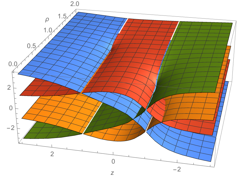
Figure 5: $U(\rho,z)$ defined by (6.10) for $\sigma_{1}=1$, $\sigma_{2}=1.5$, $\mu_{1}=1.2$, $\mu_{2}=0.5$, $z_{1}=-z_{2}=1$, and for $\rho\in[0,2]$, $z\in[-4,4]$. The four different branch sheets (different colours online) correspond to values of $U$ in four different spacetime regions.

As a result, expanding the function in (6.19) at small $\rho$ yields

$$X_{a}+iY_{a}=s(a)\left(z_{a}^{\pm}+\frac{\rho^{2}}{2z_{a}^{\pm}}+{\cal O}(\rho^{4})\right)$$ (6.21)

where $z^{\pm}_{a}$ is defined in (6.6) and $s(a)$ is given by (6.18). Using this to compute $U$ in (6.10) gives, if $s(1)=s(2)=\pm 1$,

$$U(\rho=0,z)=\pm\left\{\sigma_{1}\arctan\left(\frac{z-z_{1}}{\mu_{1}}\right)+\sigma_{2}\arctan\left(\frac{z-z_{2}}{\mu_{2}}\right)\right\},$$ (6.22)

and, if $s(1)=-s(2)=\pm 1$,

$$U(\rho=0,z)=\pm\left\{\sigma_{1}\arctan\left(\frac{z-z_{1}}{\mu_{1}}\right)-\sigma_{2}\arctan\left(\frac{z-z_{2}}{\mu_{2}}\right)\right\},$$ (6.23)

which are the values of $U$ on the four symmetry axes. This can be compared with Eqs.(5.21),(5.22) in the single ring case, in which case there are only two symmetry axes.

Let us now similarly compute the value of $k$ at the symmetry axes. The amplitudes $k_{a}$ in (6.12) are insensitive to signs of $X_{a}$, $Y_{a}$ hence for given $(\rho,z)$ their values are the same on all Weyl charts. The $k_{12}$ amplitude in (6.12) depends on products $(X_{1}+iY_{1})(X_{2}+iY_{2})$ and $(X_{1}+iY_{1})(X_{2}-iY_{2})$ for which there are two sign options. If one chooses in (6.21) $s(1)=s(2)$ then one will have for small $\rho$

$$(X_{1}+iY_{1})(X_{2}+iY_{2})=z_{1}^{+}z_{2}^{+}+{\cal O}(\rho^{2}),~{}~{}~{}~{}(X_{1}+iY_{1})(X_{2}-iY_{2})=z_{1}^{+}z_{2}^{-}+{\cal O}(\rho^{2}),$$

inserting which to (6.11),(6.12) gives

$$k_{1}(0,z)=k_{2}(0,z)=k_{12}(0,z)=0.$$ (6.24)

   

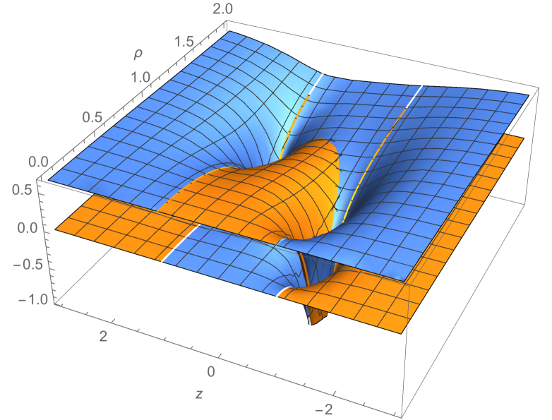
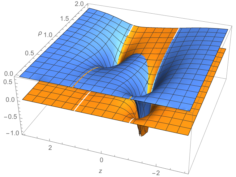
Figure 6: $k(\rho,z)$ defined by (6.10) for the same parameter values as in Fig.5 and for $\rho\in[0,2]$, $z\in[-4,4]$. It shows only two sheets made of (blue and yellow online) branches computed from $X_{a},Y_{a}$ chosen either as in (6.16) (left panel) or as in (6.19) (right panel). The resulting sheets are the same in both cases.

The other possibility is to chose in (6.21) $s(1)=-s(2)$, then one has at small $\rho$

$$(X_{1}+iY_{1})(X_{2}+iY_{2})=-\left({z}_{1}^{+}+\frac{\rho^{2}}{2z_{1}^{+}}\right)\left(z_{2}^{+}+\frac{\rho^{2}}{2z_{2}^{+}}\right)+{\cal O}(\rho^{4}),$$

$$(X_{1}+iY_{1})(X_{2}-iY_{2})=-\left({z}_{1}^{+}+\frac{\rho^{2}}{2z_{1}^{+}}\right)\left(z_{2}^{-}+\frac{\rho^{2}}{2z_{2}^{-}}\right)+{\cal O}(\rho^{4}).$$ (6.25)

Inserting this to (6.11),(6.12) gives

$$k_{1}(0,z)=k_{2}(0,z)=0,$$ (6.26)

but $k_{12}$ assumes a constant non-zero value

$$k_{12}(0,z)=\ln\left(\frac{(z_{1}-z_{2})^{2}+(\mu_{1}-\mu_{2})^{2}}{(z_{1}-z_{2})^{2}+(\mu_{1}+\mu_{2})^{2}}\right).$$ (6.27)

The conclusion is that $k(\rho,z)$ vanishes at the two symmetry axes with $s(1)=s(2)$ where $U$ is given by (6.22), hence these two axes are regular. However, $k$ assumes the constant non-zero value (6.27) everywhere at the other two axes, where $s(1)=-s(2)$ and $U$ is given by (6.22). Hence these two axes are singular and contain infinite struts (see Fig.6). Therefore, two of the four symmetry axes of the solution are regular while the other two are everywhere singular.

The two-wormhole system was first discussed in [22], where the solution for $U(\rho,z)$ was obtained (see also [53]). It took next more than 30 years to obtain also the explicit solution for $k(\rho,z)$ and not just the integral representation (3.3) [24]. The formula (6.27) was also obtained in [24], however, it was concluded there that $k(0,z)$ is discontinuous and assumes the value (6.27) either inside the interval $[z_{1},z_{2}]$ while vanishing outside, or the other way round. As one can see in Fig.6 (left panel) precisely this type of behaviour is shown separately by the two (blue and yellow online) solution branches. However, $k$ is clearly continuous on the combined surface made of both branches. Moreover, choosing regular near the axis amplitudes $X_{a},Y_{a}$ (6.19) renders $k(0,z)$ constant for each separate branch, as one can see in the right panel of Fig.6. In any case, since $U$ is everywhere finite and smooth, the field equations imply that the derivative $\partial_{z}k\sim\rho$ should vanish at the axis hence $k(0,z)$ cannot jump.

6.2 Locally flat wormholes

Summarising the above discussion, the oblate vacuum solutions obtained from the two-rod metrics describe a pair of wormholes. An analysis similar to that in Section (5.2.2) above shows that their curvature exhibits the conical and power-law singularities at the two circles $(\rho,z)=(\mu_{a},z_{a})$, which can be viewed as the positions of singular matter sources – two negative tension rings. In addition, the solutions show a conical singularity everywhere at the two of their four symmetry axes where the function $k$ assumes a constant non-zero value. Therefore, these solutions are singular even at infinity.

There is, however, a notable exception obtained by taking in (6.10) the $\sigma_{1}\to 0$ and $\sigma_{2}\to 0$ limit, which gives $U=k=0$ everywhere, hence the metric becomes locally flat. The conical singularity along the $z$-axes as well as the power-law curvature singularity at the rings then disappear. However, the topology remains non-trivial as one still needs four Weyl charts to cover the manifold, hence the conical singularities at the points $(\mu_{a},z_{a})$ of the $(\rho,z)$ plane remain (we now assume without loss of generality that $\mu_{a}>0$ since in the opposite case one should simply replace in all formulas below $\mu_{a}$ by $|\mu_{a}|$). For example, a contour around the point $(\mu_{1},z_{1})$ in the $D^{+}_{+}$ patch shown in Fig.7 does not close after the first revolution since when arriving at the lower edge of the cut it passes to the $D^{-}_{+}$ patch and only after a second revolution returns back to the $D^{+}_{+}$ patch to close.

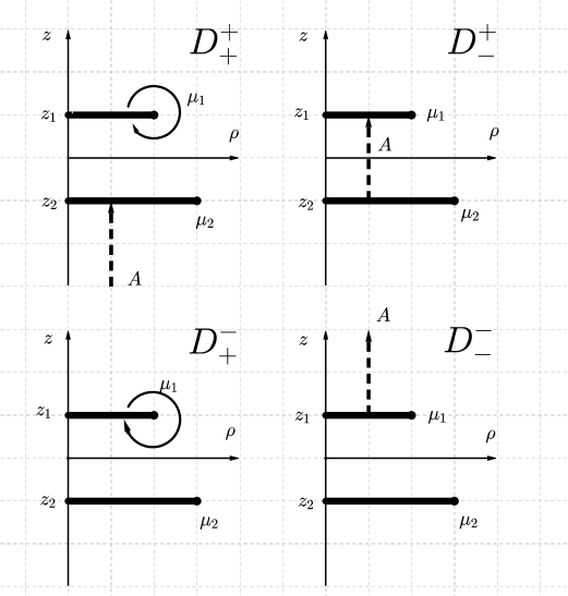
Figure 7: The two-ring wormhole is covered by four Weyl charts, each having two branch cuts. The upper cuts on $D^{+}_{\pm}$ and $D^{-}_{\pm}$ are glued to each other such that the upper edge of the one is identified with the lower edge of the other and vice-versa; similarly for the lower cuts on $D^{\pm}_{+}$ and $D^{\pm}_{-}$. As a result, the geodesic $A$ crosses several charts.

Therefore, the total angle increment is $4\pi$ hence there is an angle deficit of $-2\pi$ corresponding to a cosmic string of negative tension $T=-c^{4}/(4G)$. This string stretches in the $\varphi$-direction, hence this is a ring of radius $\mu_{1}$ placed at $z=z_{1}$. Similar argument shows that there is also a ring of the same tension and of radius $\mu_{2}$ placed at $z=z_{2}$. Therefore, the solution is sourced by a pair of negative tension rings whose positions and radii can be arbitrary.

Since the metric is locally flat, the geodesics are simply straight lines. Those initially parallel to the $z$-axis will always remain parallel to it, which helps to understand once again why there are four symmetry axes. Consider a geodesic which is close enough to the axis to thread both rings, as for example the geodesic $A$ in Fig.7 which stars at the $D^{+}_{+}$ chart at $z=-\infty$. When it threads the ring at $z=z_{2}$ it passes to the $D^{+}_{-}$ chart and continues there, until it threads the second ring at $z=z_{1}$ and passes to the $D^{-}_{-}$ chart where it stays till reaching $z=+\infty$. Therefore, this geodesic follows the pattern

$$D^{+}_{+}\to D^{+}_{-}\to D^{-}_{-}\,$$ (6.28)

which determines one of the four $z$-axes of the solution. Similarly, a geodesic which starts on $D^{-}_{-}$ and follows the $z$-axis proceeds as

$$D^{-}_{-}\to D^{-}_{+}\to D^{+}_{+}\,$$ (6.29)

which determines the second axis. The other two axes are similarly defined by

$$D^{+}_{-}\to D^{+}_{+}\to D^{-}_{+}\,,~{}~{}~{}~{}~{}~{}~{}D^{-}_{+}\to D^{-}_{-}\to D^{+}_{-}\,.$$ (6.30)

The above arguments can be straightforwardly generalized to the case of $N$ rings of arbitrary radii $\mu_{a}$ and positions $z_{a}$ and of the same tension $T=-c^{4}/(4G)$. The metric expressed in Weyl coordinates is manifestly flat but the topology is non-trivial and one needs $2^{N}$ Weyl charts

$$D_{s(1)s(2)\ldots s(N)}:\{\rho\geq 0,-\infty<z<\infty\}$$ (6.31)

to cover the whole of the manifold. Here $s(a)=\pm 1$ and each chart has $N$ cuts

$${\cal I}_{a}=\left\{\rho\in[0,\mu_{a}],z=z_{a}\right\},~{}~{}~{}~{}a=1,\ldots N.$$ (6.32)

The atlas is obtained by gluing together the $m$-th cuts on all pairs of charts with coinciding indices $s(a\neq m)$. For example, the upper edge of the first cut on $D_{+s(2)\ldots s(N)}$ should be identified with the lower edge of the first cut on $D_{-s(2)\ldots s(N)}$ and vise versa for all possible values of $s(2),\ldots s(N)$. This gives an exact solution of Einstein equations sourced by $N$ singular rings whose geometry is everywhere flat except at the ring positions.

6.3 Solutions with scalar field

Any of the discussed above vacuum Weyl metrics described by

$$(U,k,\Phi=0)$$ (6.33)

can be promoted to solutions with $\Phi\neq 0$. Applying symmetries (3.8) and (3.9) gives solutions with the conventional scalar,

$$U_{s}=\frac{1}{s}\,U,~{}~{}~{}~{}~{}k_{s}=k,~{}~{}~{}~{}\phi_{s}=\frac{\sqrt{s^{2}-1}}{s}\,U,~{}~{}~{}~{}s\geq 1,$$ (6.34)

boosted solutions with phantom field,

$$U_{s}=\frac{1}{s}\,U,~{}~{}~{}~{}~{}k_{s}=k,~{}~{}~{}~{}\psi_{s}=\frac{\sqrt{1-s^{2}}}{s}\,U,~{}~{}~{}~{}s\leq 1,$$ (6.35)

and their swapped version

$$U_{s}=\frac{1}{s}\,U,~{}~{}~{}~{}~{}k_{s}=-k,~{}~{}~{}~{}\psi_{s}=\frac{\sqrt{1+s^{2}}}{s}\,U,~{}~{}~{}~{}s\in(-\infty,\infty).$$ (6.36)

Since the original solution can exist in prolate and oblate versions, this gives six one-parameter families of solutions with scalar. In addition, twice as many solutions can be obtained by acting on (6.34)–(6.36) with the tachyon symmetry (3.13).

For example, taking the two-wormhole vacuum metric (6.10), applying the swap symmetry (6.36), and then taking the limit $s\to\infty$ gives the two-wormhole counterpart of the ultrastatic solution of Bronnikov and Ellis. This solution is no longer spherically symmetric and it contains infinite struts along two symmetry axes.

More generally, all solutions with $\Phi\neq 0$ obtained from the two-rod metrics are singular since already their prolate and oblate vacuum versions have struts. The only solutions without struts are the vacuum rings with $U=k=0$, but symmetries (6.34)–(6.36) act trivially in this case and give $\Phi=0$.

7 Solutions from point masses – Appell wormhole

Let us finally discuss solutions obtained from the Chazy-Curzon metric (4.14),(4.3). This metric does not admit the “prolate” and “oblate” generalizations since the scale symmetry $(U,k)\to(\lambda U,\lambda^{2}k)$ acts trivially only redefining the parameter $m$ in (4.14). Hence, there is only one vacuum solution,

$$U=-\frac{m}{R}\,,\qquad k=-\frac{m^{2}\rho^{2}}{2R^{4}}\,,$$ (7.1)

with $R=\sqrt{\rho^{2}+z^{2}}$, inserting which to (6.34)–(6.36) gives solutions with scalar field.

More possibilities exist for the two mass solution (4.3) because it contains three free parameters, $m_{\pm}$ and $m$. Applying $(U,k)\to(\lambda U,\lambda^{2}k)$ again results in a trivial rescaling of $m_{\pm}$, but this time there is a non-trivial possibility to complexify via

$$m\to i\mu,~{}~{}~{}~{}~{}~{}m_{\pm}\to-\frac{M}{2}\,e^{\pm i\eta}\,,$$ (7.2)

with constant and real $\mu,M,\eta$. This gives

$$R_{\pm}=\sqrt{\rho^{2}+(z\pm m)^{2}} \to \sqrt{\rho^{2}+(z\pm i\mu)^{2}}=X\pm iY=x\pm i\mu\cos\vartheta\equiv{\cal R}e^{\pm i{\cal S}}~{}~{}$$ (7.3)

with ${\cal R}=\sqrt{X^{2}+Y^{2}}$ and $\tan({\cal S})={Y}/{X}$ where $X,Y$ in terms of $\rho,z$ are given by (5.10). Applying this to (4.3) gives the real-valued solution,

$$U=\frac{M}{\cal R}\,\cos({\cal S}-\eta),~{}~{}~{}~{}k=-\frac{M^{2}\rho^{2}}{4{\cal R}^{4}}\,\cos(4{\cal S}-2\eta)-\frac{M^{2}}{8\mu^{2}}\left(\frac{\rho^{2}+z^{2}+\mu^{2}}{{\cal R}^{2}}-1\right).$$ (7.4)

This is regular at the symmetry axis, $k(0,z)=0,$ and describes the so called Appell ring whose Newtonian potential $U$ [59] is produced by a disk of negative mass density whose rim has positive mass density [62, 63, 64]. Since the phase ${\cal S}$ is double-valued around the branching point $(\rho,z)=(\mu,0)$, the solution has the same double-sheeted topology as the considered above wormholes. Hence this is again a wormhole. However, since ${\cal R}$ vanishes at the ring, the Newtonian potential diverges [64].

Taking as the pair $(U,k)$ either the original Chazy-Curzon solution (4.3) or the Appell ring (7.4) and injecting to (6.34)–(6.36) gives solutions with scalar field. In particular, applying to (7.4) the boost (6.35) and then taking the infinite boost limit $s\to 0$ while keeping constant the ratio ${M}/{s}\equiv A$ yields $k=0$ and

$$U=\psi=A\,\frac{\cos({\cal S}-\eta)}{\cal R}=A\cos\eta\,\frac{x}{x^{2}+\mu^{2}\cos^{2}\vartheta}+A\mu\sin\eta\,\frac{\cos\vartheta}{x^{2}+\mu^{2}\cos^{2}\vartheta}.$$ (7.5)

For $\eta=\pi/2$ this reduces to the ring solution of [60, 61] discussed around Eq.(5.51).

8 Conclusions

To recapitulate, we applied above the duality rotations to the vacuum Weyl metrics to produce new solutions with scalar field. We were mainly interested in the wormhole solutions with several asymptotically flat regions. Such solutions are best known in systems with exotic matter, but it is little known that they exist also in vacuum GR, being sourced by thin negative tension rings. The one-ring solutions show a conical singularity and a power-law curvature singularity at the ring, but the Newtonian potential is finite everywhere. In this respect, the ring wormholes differ from other known solutions with rings/strings which show infinite red or blue shifts or pathologies like closed timelike curves. These are, for example, the Kerr black hole containing inside the horizon a ring singularity which can also be viewed as a wormhole [65], or the Appell ring considered above (see [64] for other singular rings), or the NUT wormholes containing inside a singular Misner string [66, 67].

The vacuum ring wormholes could be viewed as “primary” while solutions with scalar field are obtainable from them via duality rotations. This gives rings “dressed with scalar”, conventional or phantom. In particular, the spherically symmetric BE wormhole can be obtained by dressing the ring with the phantom field. As we have seen, one can construct large families of such “dressed up” solutions.

The most interesting property of our ring wormholes is that, unlike other known rings, they admit a remarkable limit where their geometry becomes locally flat – when the tension of all rings attains the value $T=-c^{4}/(4G)$. The topology then remains non-trivial and shows several interconnected asymptotic regions. Solutions then become regular everywhere apart from the rings where they show a mild conical singularity, which could presumably be smoothened by replacing the thin rings by regular toroidal sources of finite thickness. Such rings literally cut holes in flat space.

In some parts of our discussion we summarised and generalised little known facts scattered in the literature, whereas other parts are original, as for example the description of the “scalar-dressed” solutions obtained via duality transformations and of the ring and multi-ring solutions with locally flat geometry. The main message we were trying to convey is that traversable wormholes could be less exotic objects than is usually thought, since they exist already in vacuum GR and not necessarily only in systems with exotic matter.

Appendix A Isometric embeddings of the BE wormhole

Introducing $(X_{1},X_{2},X_{3})=\sqrt{x^{2}+\mu^{2}}\,(\sin\vartheta\cos\varphi,\sin\vartheta\sin\varphi,\cos\vartheta)$ and also $Z$,

$$dZ=\frac{\mu}{\sqrt{x^{2}+\mu^{2}}}\,dx~{}~{}~{}~{}~{}\Rightarrow~{}~{}~{}~{}~{}x=\sinh\left(\frac{Z}{\mu}\right),$$ (A.1)

the ultrastatic BE solution (2.16) can be represented as the geometry induced on a hypersurface in five dimensional Minkowski space,

$$ds^{2}=-dt^{2}+dx^{2}+(x^{2}+\mu^{2})d\Omega^{2}=-dt^{2}+dX_{1}^{2}+dX_{2}^{2}+dX_{3}^{2}+dZ^{2}\,,$$ (A.2)

where

$$X_{1}^{2}+X_{2}^{2}+X_{3}^{2}=\mu^{2}\cosh^{2}\left(\frac{Z}{\mu}\right).$$ (A.3)

 

Figure 8: Embedding of the equatorial section of the BE wormhole to the 3-dimensional Euclidean space spanned by $X_{1},X_{2},Z$ defined by (A.4),(A.5).

It follows that the spatial 2-geometry of the equatorial plane $X_{3}=0$ is a catenoid (see Fig.8) – a surface of revolution in three-dimensional Euclidean space with the line element

$$dX_{1}^{2}+dX_{2}^{2}+dZ^{2}=dr^{2}+r^{2}d\varphi^{2}+dZ^{2}$$ (A.4)

whose meridional curve is the catenary,

$$r=\mu\cosh\left(\frac{Z}{\mu}\right).$$ (A.5)

One can also construct the embedding of the non-ultrastatic BE geometry (2.1.3),

$$ds^{2}=-A^{2}(x)dt^{2}+\frac{dx^{2}}{B^{2}(x)}+r^{2}(x)(d\vartheta^{2}+\sin^{2}\vartheta d\varphi^{2})$$ (A.6)

with

$$A(x)=B(x)=e^{\Psi/s},~{}~{}~{}~{}~{}~{}~{}r(x)=\frac{\sqrt{x^{2}+\mu^{2}}}{B(x)},~{}~{}~{}~{}~{}~{}\Psi=\arctan\left(\frac{x}{\mu}\right),$$ (A.7)

following the procedure of [68, 69]. This geometry can be embedded into the 7-dimensional Minkowski space with the metric

$$ds^{2}=-dX_{0}^{2}+dX_{1}^{2}+dX_{2}^{2}+dX_{3}^{2}+dX_{4}^{2}+dX_{5}^{2}-dX_{6}^{2}$$ (A.8)

by the following explicit formulas for $X_{k}=X_{k}(t,x,\vartheta,\varphi)$:

$$X_{0} = A(x)\sinh(t),~{}~{}~{}~{}~{}~{}X_{1}=A(x)\cosh(t),~{}~{}~{}~{}~{}~{}~{}$$

$$X_{2} = r(x)\sin\vartheta\cos\varphi,~{}~{}~{}X_{3}=r(x)\sin\vartheta\sin\varphi,~{}~{}~{}X_{4}=r(x)\cos\vartheta,~{}~{}~{}~{}$$

$$X_{5} = \int\frac{dx}{B(x)},~{}~{}~{}~{}~{}~{}X_{6}=\int\sqrt{A^{\prime 2}(x)+r^{\prime 2}(x)}\,dx\,,$$ (A.9)

where the prime denotes the derivative with respect to $x$.

Appendix B Flamm embedding versus Einstein-Rosen bridge

It is instructive to discuss the relation between the work of Flamm [2] of 1916 and analysis of Einstein and Rosen [1] of 1935 presenting the first ever example of wormholes.

Flamm (see [3],[4] for the English translation) was the first to consider isometric embeddings of the Schwarzschild solution. Specifically, the spatial part of the vacuum Schwarzschild metric in the $r>2M$ region can be represented as

$$dl^{2}=\frac{dr^{2}}{1-2M/r}+r^{2}d\Omega^{2}=dr^{2}+r^{2}d\Omega^{2}+dZ^{2}$$ (B.1)

where

$$dZ^{2}=\frac{dr^{2}}{{r/(2M)-1}}~{}~{}~{}~{}~{}\Rightarrow~{}~{}~{}~{}~{}r=r(Z)\equiv 2M+\frac{Z^{2}}{8M}.$$ (B.2)

   

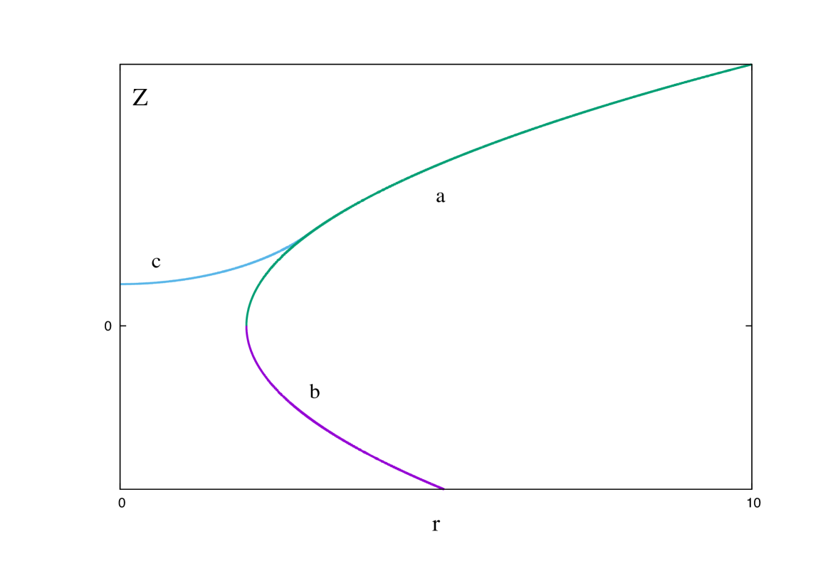
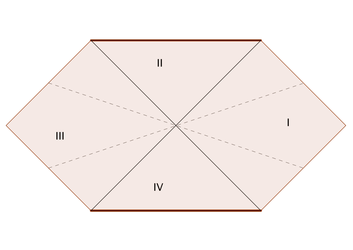
Figure 9: Left: the Flamm embedding – the surface obtained by rotating the curve $c$ (interior region) and the smoothly joining it part of the curve $a$ (exterior region) around the $Z$-axis. Right: the Einstein-Rosen coordinates $t,Z$ covering the $I+III$ regions of the Kruskal manifold. $Z$ varies from $-\infty$ to $+\infty$ along the dashed lines of constant $t$. The bridge is at the central $Z=0$ point joining the two regions.

Therefore, the geometry is the same as that induced on the paraboloid of revolution obtained by rotating the parabola $r=r(Z)$ around the Z-axis of the four-dimensional Euclidean space. The parabola consists of two parts denoted by $a$ and $b$ in Fig.9 which belong, respectively, to the $Z>0$ and $Z<0$ regions. Since the $a$-part is enough to cover the $r>2M$ region, Flamm retains only this curve. It smoothly matches at a point $r=r_{0}>2M$ the curve $c$ describing the embedding of the interior solution with a matter source in the $r<r_{0}$ region (see Fig.9). Therefore, the surface obtained by rotating the curves $a+c$ in Fig.9 around the Z-axis has the same 3-geometry as that for the combined exterior+interior Schwarzschild solution. The curve $b$ in Fig.9 can be disregarded in this case.

Einstein and Rosen (ER) [1] did not refer to Flamm but their construction can be easily understood using Flamm’s analysis. Specifically, they retain the curve $b$ but disregard the $r<2M$ region by setting in the line element $r=r(Z)$ with $Z\in(-\infty,+\infty)$ becoming the radial coordinate (they actually use the variable $u=Z/\sqrt{8M}$). Rotating the full parabola $a+b$ around the $Z$-axis then gives a surface similar to the wormhole shown in Fig.8. Using the modern formulation in terms of the Kruskal extension, the ER coordinates cover the $I$ and $III$ regions of the conformal diagram shown in Fig.9. These two exterior parts are connected by the bridge (wormhole thorat) – the surface of minimal radius $r(0)=2M$ corresponding to the central point of the diagram (the Boyer axis). The bridge cannot be traversed by ordinary matter because intervals between points in region $I$ and those in region $III$ are spacelike.

One should stress that, although the 3-metric is regular, the full 4-metric

$$ds^{2}=-\frac{Z^{2}}{16M^{2}+Z^{2}}\,dt^{2}+\left(1+\frac{Z^{2}}{16M^{2}}\right)dZ^{2}+4M^{2}\left(1+\frac{Z^{2}}{16M^{2}}\right)^{2}d\Omega^{2}$$ (B.3)

degenerates at $Z=0$ hence the ER coordinates are not global. At the same time, replacing $Z^{2}\to Z^{2}+\alpha^{2}$ with a small constant $\alpha$ in the numerator of $g_{00}$ would produce a globally static solution with a thin shell of matter around $Z=0$ resembling a thin shell wormhole in modern language. This is similar to some ideas expressed in the ER paper.

Contrary to what one often sees in the literature, the Flamm-ER 3-surface does not become flat for $r\to\infty$ since its meridional parabola does not have a linear asymptote.

References

- [1] A. Einstein and N. Rosen, The particle problem in the General Theory of Relativity, Phys.Rev. 48 (1935) 73–77.
- [2] L. Flamm, Beitraege zur Einsteinschen Gravitationstheorie, Zeit.Phys. XVII (1916) 448–454.
- [3] L. Flamm, Contributions to Einstein’s theory of gravitation, Gen.Rel.Grav. 47 (2015) 72.
- [4] G. W. Gibbons, Editorial note to: Ludwig Flamm, Contributions to Einstein’s theory of gravitation, Gen.Rel.Grav. 47 (2015) 71.
- [5] A. Einstein, B. Podolsky and N. Rosen, Can quantum mechanical description of physical reality be considered complete?, Phys.Rev. 47 (1935) 777–780.
- [6] J. Maldacena and L. Susskind, Cool horizons for entangled black holes, Fortsch.Phys. 61 (2013) 781–811, [1306.0533].
- [7] C. W. Misner and J. A. Wheeler, Classical physics as geometry: Gravitation, electromagnetism, unquantized charge, and mass as properties of curved empty space, Annals Phys. 2 (1957) 525–603.
- [8] C. W. Misner, Wormhole Initial Conditions, Phys.Rev. 118 (1960) 1110–1111.
- [9] M. Cvetic, G. W. Gibbons and C. N. Pope, Super-Geometrodynamics, JHEP 03 (2015) 029, [1411.1084].
- [10] Virgo, LIGO Scientific collaboration, B. P. Abbott et al., Observation of Gravitational Waves from a Binary Black Hole Merger, Phys.Rev.Lett. 116 (2016) 061102, [1602.03837].
- [11] M. Morris, K. Thorne and U. Yurtsever, Wormholes, time machines, and the weak energy condition, Phys.Rev.Lett. 61 (1988) 1446–1449.
- [12] M. Visser, Lorentzian wormholes: From Einstein to Hawking. AIP, 1996.
- [13] S. W. Hawking and G. F. R. Ellis, The Large Scale Structure of Space-Time. Cambridge Monographs on Mathematical Physics. Cambridge University Press, 2011, 10.1017/CBO9780511524646.
- [14] J. L. Friedman, K. Schleich and D. M. Witt, Topological censorship, Phys.Rev.Lett. 71 (1993) 1486–1489, [gr-qc/9305017].
- [15] D. Hochberg and M. Visser, The null energy condition in dynamic wormholes, Phys.Rev.Lett. 81 (1998) 746–749, [gr-qc/9802048].
- [16] K. Bronnikov, Scalar-tensor theory and scalar charge, Acta Phys.Polon. B4 (1973) 251–266.
- [17] H. G. Ellis, Ether flow through a drainhole - a particle model in general relativity, J.Math.Phys. 14 (1973) 104–118.
- [18] P. Kanti, B. Kleihaus and J. Kunz, Wormholes in Dilatonic Einstein-Gauss-Bonnet Theory, Phys.Rev.Lett. 107 (2011) 271101, [1108.3003].
- [19] K. Bronnikov and S.-W. Kim, Possible wormholes in a brane world, Phys.Rev. D67 (2003) 064027, [gr-qc/0212112].
- [20] S. V. Sushkov and R. Korolev, Scalar wormholes with nonminimal derivative coupling, Class.Quant.Grav. 29 (2012) 085008, [1111.3415].
- [21] S. V. Sushkov and M. S. Volkov, Giant wormholes in ghost-free bigravity theory, JCAP 1506 (2015) 017, [1502.03712].
- [22] G. Clement, Axisymmetric regular multiwormhole solutions in five-dimensional General Relativity, Gen.Rel.Grav. 16 (1984) 477.
- [23] H. Weyl, The theory of gravitation, Annalen Phys. 54 (1917) 117–145.
- [24] G. Cl ment, Axisymmetric multiwormholes revisited, Gen.Rel.Grav. 48 (2016) 76, [1511.06249].
- [25] G. Clement, Regular multiparticle solutions of Einstein-Maxwell scalar field theories, Class.Quant.Grav. 1 (1984) 275.
- [26] G. Clement, A class of stationary axisymmetric solutions of Einstein-Maxwell scalar field theories, Class.Quant.Grav. 1 (1984) 283.
- [27] G. Clement, A class of wormhole solutions to higher dimensional General Relativity, Gen.Rel.Grav. 16 (1984) 131.
- [28] A. Chodos and S. L. Detweiler, Spherically symmetric solutions in five-dimensional General Relativity, Gen.Rel.Grav. 14 (1982) 879.
- [29] D. Zipoy, Topology of some spheroidal metrics, J.Math.Phys. 7 (1966) 1137–1143.
- [30] K. A. Bronnikov and J. C. Fabris, Weyl space-times and wormholes in D-dimensional Einstein and dilaton gravity, Class.Quant.Grav. 14 (1997) 831–842.
- [31] G. Clement, Selfgravitating cosmic rings, Phys.Lett. B449 (1999) 12–16, [gr-qc/9808082].
- [32] G. Clement, Spinning ring wormholes: a classical model for elementary particles?, in Proceedings, 4th Alexander Friedmann International Seminar on Gravitation and Cosmology: St. Petersburg, Russia, June 17 - 25, 1998, 1998. gr-qc/9810075.
- [33] G. W. Gibbons and M. S. Volkov, Ring wormholes via duality rotations, Phys.Lett. B760 (2016) 324–328, [1606.04879].
- [34] T. Tahamtan and O. Svitek, Properties of Robinson–Trautman solution with scalar hair, Phys.Rev. D94 (2016) 064031, [1603.07281].
- [35] I. Z. Fisher, Scalar mesostatic field with regard for gravitational effects, Zh.Eksp.Teor.Fiz. 18 (1948) 636–640, [gr-qc/9911008].
- [36] A. I. Janis, E. T. Newman and J. Winicour, Reality of the Schwarzschild Singularity, Phys.Rev.Lett. 20 (1968) 878–880.
- [37] S. Abdolrahimi and A. A. Shoom, Analysis of the Fisher solution, Phys. Rev. D81 (2010) 024035, [0911.5380].
- [38] G. W. Gibbons, Phantom matter and the cosmological constant, hep-th/0302199.
- [39] A. Peres, Gravitational field of a tachyon, Phys.Lett. A7 (1970) 361–362.
- [40] L. S. Schulman, Gravitational shock waves from tachyons, Nuov.Cim. B2 (1971) 38–44.
- [41] J. R. Gott, Tachyon singularity - a spacelike counterpart of the Schwarzschild black hole, Nuov.Cim. B22 (1974) 49–69.
- [42] G. W. Gibbons and D. A. Rasheed, Dyson pairs and zero mass black holes, Nucl. Phys. B476 (1996) 515–547, [hep-th/9604177].
- [43] W. Israel and K. Khan, Collinear particles and Bondi dipoles in General Relativity, Nuov.Cim. XXXIII (1964) 331–344.
- [44] J. Chazy, Sur le champ de gravitation de deux masses fixées dans la théorie de la relativité, Bull.Soc.Math.France 52 (1924) 17–38.
- [45] H. Curzon, Cylindrical solutions of Einstein’s gravitational equations, Proc.Math.Soc. London 25 (1924) 477–480.
- [46] L. Silberstein, Two-Centers Solution of the Gravitational Field Equations, and the Need for a Reformed Theory of Matter, Phys.Rev. 49 (1936) 268–270.
- [47] N. Schleifer, Condition of elementary flatness and the two-particle Curzon solution, Phys.Let. A112 (1985) 204–207.
- [48] A. Papapetrou, A static solution of the equations of the gravitational fields for an arbitrary charge distribution, Proc.Roy.Irish.Acad. A51 (1947) 191.
- [49] S. D. Majumdar, A class of exact solutions of Einstein’s field equations, Phys.Rev. 72 (1947) 390–398.
- [50] B. H. Voorhees, Static axially symmetric gravitational fields, Phys.Rev. D2 (1970) 2119–2122.
- [51] H. Kodama and W. Hikida, Global structure of the Zipoy-Voorhees-Weyl spacetime and the delta=2 Tomimatsu-Sato spacetime, Class.Quant.Grav. 20 (2003) 5121–5140, [gr-qc/0304064].
- [52] G. Lukes-Gerakopoulos, The non-integrability of the Zipoy-Voorhees metric, Phys.Rev. D86 (2012) 044013, [1206.0660].
- [53] A. I. Egorov, P. E. Kashargin and S. V. Sushkov, Scalar multi-wormholes, Class.Quant.Grav. 33 (2016) 175011, [1603.09552].
- [54] C. Schiller, Simple derivation of minimum length, minimum dipole moment and lack of space-time continuity, Int. J. Theor. Phys. 45 (2006) 221–235.
- [55] G. W. Gibbons, The Maximum tension principle in general relativity, Found. Phys. 32 (2002) 1891–1901, [hep-th/0210109].
- [56] S. Krasnikov, The Quantum inequalities do not forbid space-time shortcuts, Phys. Rev. D67 (2003) 104013, [gr-qc/0207057].
- [57] M. Visser, Traversable wormholes: Some simple examples, Phys. Rev. D39 (1989) 3182–3184, [0809.0907].
- [58] T. Matos, Class of Einstein-Maxwell phantom fields: rotating and magnetised wormholes, Gen. Rel. Grav. 42 (2010) 1969–1990, [0902.4439].
- [59] P. Appell, Quelques remarques sur la théorie des potentiels multiformes, Math.Ann.Lpz. 30 (1887) 155–156.
- [60] G. Miranda, T. Matos and N. M. Garcia, Kerr-Like Phantom Wormhole, Gen. Rel. Grav. 46 (2014) 1613, [1303.2410].
- [61] T. Matos, L. A. Urena-Lopez and G. Miranda, Wormhole cosmic censorship, Gen. Rel. Grav. 48 (2016) 61, [1203.4801].
- [62] R. Gleiser and J. Pullin, Appell rings in general relativity, Class.Quant.Grav. 6 (1989) 977–985.
- [63] P. S. Letelier and S. R. Oliveira, Superposition of Weyl solutions: the equilibrium forces, Class. Quant. Grav. 15 (1998) 421–433, [gr-qc/9710122].
- [64] O. Semerák, Static axisymmetric rings in general relativity: how diverse they are, Phys.Rev. D94 (2016) 104021, [1611.03299].
- [65] B. Carter, Global structure of the Kerr family of gravitational fields, Phys.Rev. 174 (1968) 1559–1571.
- [66] G. Clément, D. Gal’tsov and M. Guenouche, NUT wormholes, Phys.Rev. D93 (2016) 024048, [1509.07854].
- [67] E. Ayon-Beato, F. Canfora and J. Zanelli, Analytic self-gravitating Skyrmions, cosmological bounces and AdS wormholes, Phys. Lett. B752 (2016) 201–205, [1509.02659].
- [68] C. Fronsdal, Completion and embedding of the Schwarzschild solution, Phys.Rev. 116 (1959) 778–781.
- [69] M. Ferraris and M. Francaviglia, An algebraic isometric embedding of Kruskal space-time, Gen.Rel.Grav. 10 (1979) 283–296.