Capacity and Normalized Optimal Detection Error in Gaussian Channels

Abstract

For vector Gaussian channels, a precise differential connection between channel capacity and a quantity termed normalized optimal detection error (NODE) is presented. Then, this C–NODE relationship is extended to continuous-time Gaussian channels drawing on a waterfilling characterization recently found for the capacity of continuous-time linear time-varying channels. In the latter case, the C–NODE relationship becomes asymptotic in nature. In either case, the C–NODE relationship is compared with the I–MMSE relationship due to Guo et al. connecting mutual information in Gaussian channels with the minimum mean-square error (MMSE) of estimation theory.

I Introduction

The central result of Guo et al. in [1] is an identity connecting mutual information in Gaussian channels with the MMSE of estimation theory. This I–MMSE relationship reads in the case of a vector Gaussian channel

$$\frac{\mathrm{d}}{\mathrm{d}\,\mathrm{snr}}I(\boldsymbol{X};\sqrt{\mathrm{snr}}\boldsymbol{H}\boldsymbol{X}+\boldsymbol{N})=\frac{1}{2}\mathrm{mmse}(\mathrm{snr}),$$ (1)

where $\mathrm{snr}\geq 0$, $\boldsymbol{N}$ is a noise vector with independent standard Gaussian components, independent of the random vector $\boldsymbol{X}$, $\mathsf{E}\|\boldsymbol{X}\|^{2}<\infty$, and $\boldsymbol{H}$ is a deterministic matrix of appropriate dimension; $\mathrm{mmse}(\mathrm{snr})$ is the MMSE in estimating $\boldsymbol{H}\boldsymbol{X}$ given

$$\boldsymbol{Y}=\sqrt{\mathrm{snr}}\boldsymbol{H}\boldsymbol{X}+\boldsymbol{N}.$$ (2)

In [2], for a particular, effectively finite-dimensional vector Gaussian channel, an identity analogous to (1) has been derived. There, the probability distribution of the input vector $\boldsymbol{X}$ depends on $\mathrm{snr}$ such that the mutual information occurring in (1) achieves capacity of the vector Gaussian channel; however, the right-hand side (RHS) of that identity differs from (half) the MMSE as given in (1). In [3], the same vector Gaussian channel as in [2] arose from a particular continuous-time Gaussian channel through discretization by optimal detection [4] of the channel output signals with the use of matched filters, following the approach in [5] for linear time-invariant channels; after a certain normalization, the aforementioned RHS has been recognized as (half) the NODE (to be defined later) of the channel output signals. In this way, a first instance of the C–NODE relationship has been encountered.

The goal of the present paper is to extend this C–NODE relationship 1) to more general vector Gaussian channels, 2) to continuous-time Gaussian channels in the form of the linear time-varying (LTV) channels considered in [6], and 3) to compare the C–NODE relationship with the I–MMSE relationship in either case.

Notation

We use natural logarithms and so the unit nat for all information measures. $\mathcal{N}(0,\theta^{2})$ is the Gaussian distribution with mean 0 and variance $\theta^{2}$. $\mathscr{S}(\mathbb{R}^{2})$ is the Schwartz space of rapidly decreasing functions on $\mathbb{R}^{2}$; $\mathscr{S}_{\geq 0}(\mathbb{R}^{2})$ is the set of all non-negative real-valued functions in $\mathscr{S}(\mathbb{R}^{2})$. $x^{+}$ denotes the positive part of $x\in\mathbb{R}$, $x^{+}=\max\{0,x\}$. For any two functions $A=A(r),B=B(r):[1,\infty)\rightarrow\mathbb{R}$ the notation $A\doteq B$ means $A(r)=B(r)+o(r^{2})$ as $r\rightarrow\infty$, where $o(\cdot)$ is the standard Landau little-o symbol (cf. [6]).

II Vector Gaussian Channels

II-A Detection, Capacity, and Parameter $\mathrm{snr}$

Consider the vector Gaussian channel

$$\boldsymbol{Y}=\boldsymbol{H}\boldsymbol{X}+\boldsymbol{N},$$ (3)

where $\boldsymbol{H}$ is a determinstic real $L\times L$ matrix and the noise vector $\boldsymbol{N}=(N_{0},\ldots,N_{L-1})^{\mathsf{T}}$ has independent random components $N_{k}\sim\mathcal{N}(0,\theta^{2}),\,k=0,\ldots,L-1,$ with the noise variance $\theta^{2}>0$, $\boldsymbol{X}=(X_{0},\ldots,X_{L-1})^{\mathsf{T}}$ is the random input vector, and $\boldsymbol{Y}=(Y_{0},\ldots,Y_{L-1})^{\mathsf{T}}$ the corresponding output. If $\boldsymbol{x}=(x_{0},\ldots,x_{L-1})^{\mathsf{T}}$ and $\boldsymbol{n}=(n_{0},\ldots,n_{L-1})^{\mathsf{T}}$ are realizations of the random vectors $\boldsymbol{X}$ and $\boldsymbol{N}$, resp., then the realization $\boldsymbol{y}=(y_{0},\ldots,y_{L-1})^{\mathsf{T}}$ of $\boldsymbol{Y}$ is determined by the equation

$$\boldsymbol{y}=\boldsymbol{H}\boldsymbol{x}+\boldsymbol{n}.$$ (4)

$\boldsymbol{H}$ has the singular value decomposition (SVD) $\boldsymbol{H}=\boldsymbol{G}\boldsymbol{\Delta}\boldsymbol{F}^{\mathsf{T}}$ with orthogonal $L\times L$ matrices $\boldsymbol{F}$ and $\boldsymbol{G}$ and a diagonal matrix $\boldsymbol{\Delta}=\mathrm{diag}(\sqrt{\lambda_{0}},\ldots,\sqrt{\lambda_{L-1}})$, where $\lambda_{0}\geq\lambda_{1}\geq\ldots\geq\lambda_{L-1}\geq 0$ are the eigenvalues of $\boldsymbol{H}^{\mathsf{T}}\boldsymbol{H}$ (counting multiplicity). Occasionally, we shall use the invertible matrix $\boldsymbol{\Delta}_{\epsilon}$ obtained from $\boldsymbol{\Delta}$ by replacing zeros on the diagonal with some $\epsilon>0$. Writing $\boldsymbol{F}=(\boldsymbol{f}_{0}\ldots\boldsymbol{f}_{L-1})$, $\boldsymbol{G}=(\boldsymbol{g}_{0}\ldots\boldsymbol{g}_{L-1})$ with the column vectors $\boldsymbol{f}_{k},\,\boldsymbol{g}_{k}$, it then holds for every (column) vector $\boldsymbol{x}\in\mathbb{R}^{L}$ that

$$\boldsymbol{H}\boldsymbol{x}=\sum_{k=0}^{L-1}\sqrt{\lambda_{k}}a_{k}\,\boldsymbol{g}_{k},$$

where $a_{k}=\langle\boldsymbol{x},\boldsymbol{f}_{k}\rangle\triangleq\boldsymbol{x}^{\mathsf{T}}\boldsymbol{f}_{k}$. Since only the coefficients $a_{k}$ carry information, the linear combination $\boldsymbol{x}=\sum_{k=0}^{L-1}a_{k}\boldsymbol{f}_{k}$ would be a suitable channel input vector. At the receiver, the perturbed vector $\boldsymbol{v}=\boldsymbol{H}\boldsymbol{x}$, $\boldsymbol{y}=\boldsymbol{v}+\boldsymbol{n},$ is passed through a bank of matched filters $\langle\,\cdot\,,\boldsymbol{g}_{k}\rangle,\,k=0,\ldots,L-1$. The matched filter output signals are $\langle\boldsymbol{y},\boldsymbol{g}_{k}\rangle=b_{k}+e_{k}$, where $b_{k}=\langle\boldsymbol{v},\boldsymbol{g}_{k}\rangle=\sqrt{\lambda_{k}}a_{k}$, and the detection errors $e_{k}=\langle\boldsymbol{n},\boldsymbol{g}_{k}\rangle=g_{k0}n_{0}+\ldots+g_{k,L-1}n_{L-1}$ are realizations of independent identically distributed Gaussian random variables $E_{k}\sim\mathcal{N}(0,\theta^{2})$. From the detected values $\hat{b}_{k}=b_{k}+e_{k}$ we get the estimates $\hat{a}_{k}=\hat{b}_{k}/\sqrt{\lambda_{k}}=a_{k}+z_{k}$ of the coefficients $a_{k}$ for the input vector $\boldsymbol{x}$, where $z_{k}$ are realizations of independent Gaussian random variables $Z_{k}\sim\mathcal{N}(0,\theta^{2}/\lambda_{k})$ (put $\theta^{2}/0=\infty$). Thus, we are led to the new vector Gaussian channel

$$\boldsymbol{Y}=\boldsymbol{X}+\boldsymbol{Z},$$ (5)

where the random components $Z_{k}$ of the noise vector $\boldsymbol{Z}=(Z_{0},\ldots,Z_{L-1})^{\mathsf{T}}$ are distributed as described. The vector Gaussian channels (3) and (5) are equivalent in the sense that for any average input energy $S$ their capacity $C(S)$ is the same. Indeed, since mutual information is invariant with respect to invertible linear transformations, we have

$$I(\boldsymbol{X};\boldsymbol{X}+\boldsymbol{Z}) =\lim_{\epsilon\rightarrow 0}I(\boldsymbol{X};\boldsymbol{X}+\boldsymbol{\Delta}_{\epsilon}^{-1}\boldsymbol{N})$$

$$=\lim_{\epsilon\rightarrow 0}I(\boldsymbol{X};\boldsymbol{\Delta}_{\epsilon}\boldsymbol{X}+\boldsymbol{N})$$

$$=I(\boldsymbol{X};\boldsymbol{\Delta}\boldsymbol{X}+\boldsymbol{N})$$ (6)

$$=I(\tilde{\boldsymbol{X}};\boldsymbol{H}\tilde{\boldsymbol{X}}+\tilde{\boldsymbol{N}}),$$

where $\tilde{\boldsymbol{X}}=\boldsymbol{F}\boldsymbol{X}$ is an arbitrary vector with the property that $\|\tilde{\boldsymbol{X}}\|\triangleq\langle\tilde{\boldsymbol{X}},\tilde{\boldsymbol{X}}\rangle^{1/2}=\|\boldsymbol{X}\|$, and $\tilde{\boldsymbol{N}}=\boldsymbol{G}\boldsymbol{N}$ has independent components $\sim\mathcal{N}(0,\theta^{2})$ (as $\boldsymbol{N}$); consequently,

$$C(S)=\max_{\mathsf{E}\|\boldsymbol{X}\|^{2}\leq S}I(\boldsymbol{X};\boldsymbol{X}+\boldsymbol{Z})=\max_{\mathsf{E}\|\tilde{\boldsymbol{X}}\|^{2}\leq S}I(\tilde{\boldsymbol{X}};\boldsymbol{H}\tilde{\boldsymbol{X}}+\tilde{\boldsymbol{N}}).$$

The capacity of the vector Gaussian channel (5) is computed by waterfilling on the noise variances [5, Th. 7.5.1]. Let $\nu_{k}^{2}=\theta^{2}/\lambda_{k},\,k=0,1,\ldots,L-1,$ be the noise variance in the $(k+1)$st subchannel of the channel (5). Precluding the trivial case $S=0$, the “water level” $\sigma^{2}$ is then uniquely determined by the condition

$$S=\sum_{k=0}^{K-1}(\sigma^{2}-\nu_{k}^{2})=\sum_{k=0}^{L-1}(\sigma^{2}-\nu_{k}^{2})^{+},$$ (7)

where $K=\max\{k\in\mathbb{N};\,\nu_{k-1}^{2}<\sigma^{2},\,k\leq L\}$ is the number of active subchannels. The capacity $C(S)$ is achieved, if the input vector $\boldsymbol{X}=(X_{0},\ldots,X_{L-1})^{\mathsf{T}}$ has independent components $X_{k}\sim\mathcal{N}(0,\sigma^{2}-\nu_{k}^{2})$ for $k=0,\ldots,K-1$ and $X_{k}=0$ else; then

$$C(S)=\sum_{k=0}^{K-1}\frac{1}{2}\ln\left(1+\frac{\sigma^{2}-\nu_{k}^{2}}{\nu_{k}^{2}}\right)=\frac{1}{2}\sum_{k=0}^{K-1}\ln(\mathrm{snr}\,\lambda_{k}),$$

where $\mathrm{snr}\triangleq\sigma^{2}/\theta^{2}$ is the signal-to-noise ratio. Since always $\mathrm{snr}\,\lambda_{0}=\sigma^{2}/\nu_{0}^{2}\geq 1,$ $\lambda_{0}^{-1}$ is the smallest feasible $\mathrm{snr}$ (assumed when $S=0$).

Remark 1

Since, in the case of $\lambda_{0}=1$, only the portion $\sigma^{2}-\theta^{2}$ contributes to the signal, $\sigma^{2}/\theta^{2}$ is, then, rather a signal plus noise-to-noise ratio; we stick to the notation “snr” to conform with [1].

II-B C–NODE Relationship in Vector Gaussian Channels

Because of Eq. (6), for the channel (5) it holds that

$$I(\boldsymbol{X};\boldsymbol{Y})=I\left(\boldsymbol{X}^{\prime};\frac{\sigma}{\theta}\boldsymbol{\Delta}\boldsymbol{X}^{\prime}+\boldsymbol{N}^{\prime}\right),$$

where $\boldsymbol{X}^{\prime}=\sigma^{-1}\boldsymbol{X}$, and $\boldsymbol{N}^{\prime}=\theta^{-1}\boldsymbol{N}$ has independent standard Gaussian components, $\boldsymbol{N}$ being the noise vector in (3). Capacity is achieved, if $\boldsymbol{X}^{\prime}=(X_{0}^{\prime},\ldots,X_{L-1}^{\prime})^{\mathsf{T}}$ has independent components $X_{k}^{\prime}\sim\mathcal{N}(0,1-\mathrm{snr}^{-1}\lambda_{k}^{-1})$ for $k=0,\ldots,K-1$ and $X_{k}^{\prime}=0$ else. Putting $\boldsymbol{X}^{\prime\prime}=\boldsymbol{F}\boldsymbol{X}^{\prime}$, we obtain

$$I(\boldsymbol{X}^{\prime};\sqrt{\mathrm{snr}}\boldsymbol{\Delta}\boldsymbol{X}^{\prime}+\boldsymbol{N}^{\prime})=I(\boldsymbol{X}^{\prime\prime};\sqrt{\mathrm{snr}}\,\boldsymbol{H}\boldsymbol{X}^{\prime\prime}+\boldsymbol{N}^{\prime\prime}),$$ (8)

where $\boldsymbol{N}^{\prime\prime}=\boldsymbol{G}\boldsymbol{N}^{\prime}$ has independent standard Gaussian components, independent of $\boldsymbol{X}^{\prime\prime}$. Capacity is achieved, if $\boldsymbol{X}^{\prime\prime}=\boldsymbol{F}\boldsymbol{X}^{\prime}$ where $\boldsymbol{X}^{\prime}$ is distributed as above. Since the RHS of Eq. (8) then only depends on $\mathrm{snr}$, we may write (with slight abuse of notation)

$$C(\mathrm{snr}) =I(\boldsymbol{X}^{\prime\prime};\sqrt{\mathrm{snr}}\,\boldsymbol{H}\boldsymbol{X}^{\prime\prime}+\boldsymbol{N}^{\prime\prime})$$ (9)

$$=\frac{1}{2}\sum_{k=0}^{K-1}\ln(\mathrm{snr}\,\lambda_{k}).$$ (10)

The RHS of Eq. (9) is reminescent of the mutual information occurring in the I–MMSE relationship (1). It is therefore tempting to take the derivative of the RHS of Eq. (10) with respect to $\mathrm{snr}$. Before doing so, observe that $K$ depends on $\mathrm{snr}$ since $K=K(\mathrm{snr})=\max\{k\in\mathbb{N};\,\lambda_{k-1}>\mathrm{snr}^{-1},k\leq L\}$ (put $\max\emptyset=0$); on the other hand, $K(\mathrm{snr})$ is piecewise constant. Excluding those $\mathrm{snr}$’s where $K(\mathrm{snr})$ makes a jump, we thus obtain

$$\frac{\mathrm{d}}{\mathrm{d}\,\mathrm{snr}}C(\mathrm{snr})=\frac{1}{2}\frac{K}{\mathrm{snr}}=\frac{1}{2}\frac{K\theta^{2}}{\sigma^{2}}=\frac{1}{2}K(\theta/\sigma)^{2}.$$

Due to the application of matched filters for detection, optimal detection has been performed [4]. Therefore, $K\theta^{2}$ is the (total) optimal detection error; division by $\sigma^{2}$ may be regarded as a normalization. Likewise, after normalization $\sigma^{2}\rightarrow 1,\,\theta^{2}\rightarrow(\theta/\sigma)^{2}$ (retaining the $\mathrm{snr}$), $K(\theta/\sigma)^{2}$ would be the (total) optimal detection error. Anyway, the following definition appears appropriate:

Definition 1

For any feasible $\mathrm{snr}$, the NODE in the vector Gaussian channel (3) is given by the function

$$\mathrm{node}(\mathrm{snr})=\frac{K(\mathrm{snr})}{\mathrm{snr}}=K(\mathrm{snr})\,\theta^{\prime 2},$$

where $\theta^{\prime 2}\triangleq(\theta/\sigma)^{2}$ is called the primitive NODE. If $\mathrm{snr}$ is infeasible, we put formally $\mathrm{node}(\mathrm{snr})=0$.

Note that for any feasible $\mathrm{snr}$, $\mathrm{snr}^{-1}$ is identical to the primitive NODE $\theta^{\prime 2}$; so, no further normalization is needed when working with $\mathrm{snr}^{-1}$ (or $\mathrm{snr}$) in the feasible case.

Theorem 1

For all $\mathrm{snr}>\lambda_{0}^{-1}$ but for at most $L-1$ exceptions, the capacity $C(\mathrm{snr})$ of the vector Gaussian channel (3) is differentiable and satisfies

$$\frac{\mathrm{d}}{\mathrm{d}\,\mathrm{snr}}C(\mathrm{snr})=\frac{1}{2}\mathrm{node}(\mathrm{snr}).$$ (11)

Proof:

For growing $\mathrm{snr}$, differentiability breaks down when a new subchannel is added. This occurs as soon as $\lambda_{K}$ ($K$ being the actual number of subchannels) exceeds $\mathrm{snr}^{-1}$, which happens at most $L-1$ times. The rest of the theorem has already been proved. ∎

We observe a striking similarity between the I–MMSE relationship (1) and the C–NODE relationship (11). Note that the part of the estimation error in (1) is taken by a detection error in (11).

II-C Comparison of the NODE With the MMSE in Vector Gaussian Channels

To understand the difference between Eq. (1) and Eq. (11) in more detail, we calculate the MMSE. Following [1], given

$$\boldsymbol{Y}=\sqrt{\mathrm{snr}}\boldsymbol{H}\boldsymbol{X}^{\prime\prime}+\boldsymbol{N}^{\prime\prime},$$ (12)

the MMSE in estimating $\boldsymbol{H}\boldsymbol{X}^{\prime\prime}$ is

$$\mathrm{mmse}(\mathrm{snr}) =\mathsf{E}\left\|\boldsymbol{H}\boldsymbol{X}^{\prime\prime}-\boldsymbol{H}\widehat{\boldsymbol{X}^{\prime\prime}}\right\|^{2}$$

$$=\mathrm{tr}[\boldsymbol{H}(\boldsymbol{\Sigma}^{\prime\prime-1}+\mathrm{snr}\,\boldsymbol{H}^{\mathsf{T}}\boldsymbol{H})^{-1}\boldsymbol{H}^{\mathsf{T}}],$$

where $\widehat{\boldsymbol{X}^{\prime\prime}}$ is the minimum mean-square estimate of $\boldsymbol{X}^{\prime\prime}$, and $\boldsymbol{\Sigma}^{\prime\prime-1}$ is the inverse of the covariance matrix $\boldsymbol{\Sigma}^{\prime\prime}$ of $\boldsymbol{X}^{\prime\prime}$ which is given by

$$\boldsymbol{\Sigma}^{\prime\prime}=\mathsf{E}[\boldsymbol{X}^{\prime\prime}\boldsymbol{X}^{\prime\prime\mathsf{T}}]=\mathsf{E}[\boldsymbol{F}\boldsymbol{X}^{\prime}\boldsymbol{X}^{\prime\mathsf{T}}\boldsymbol{F}^{-1}]=\boldsymbol{F}\boldsymbol{\Sigma}^{\prime}\boldsymbol{F}^{-1},$$

where $\boldsymbol{\Sigma}^{\prime}=\mathsf{E}[\boldsymbol{X}^{\prime}\boldsymbol{X}^{\prime\mathsf{T}}]$ is the covariance matrix of $\boldsymbol{X}^{\prime}$. If $\boldsymbol{X}^{\prime}$ has independent Gaussian components $X_{k}^{\prime}\sim\mathcal{N}(0,1-\mathrm{snr}^{-1}\lambda_{k}^{-1}),\,k=0,\ldots,K-1,$ and $K=L$ (as assumed), then $\boldsymbol{\Sigma}^{\prime}=\mathrm{diag}(1-\mathrm{snr}^{-1}\lambda_{k}^{-1},\,k=0,\ldots,K-1)$. We now compute

$$\mathrm{mmse}(\mathrm{snr})= \;\mathrm{tr}[\boldsymbol{G}\boldsymbol{\Delta}\boldsymbol{F}^{-1}(\boldsymbol{F}\boldsymbol{\Sigma}^{\prime-1}\boldsymbol{F}^{-1}\!+\mathrm{snr}\,\boldsymbol{F}\boldsymbol{\Delta}^{2}\boldsymbol{F}^{-1})^{-1}$$

$$\;\cdot\,\boldsymbol{F}\boldsymbol{\Delta}\boldsymbol{G}^{-1}]$$

$$= \;\mathrm{tr}[\boldsymbol{G}\boldsymbol{\Delta}(\boldsymbol{\Sigma}^{\prime-1}+\mathrm{snr}\,\boldsymbol{\Delta}^{2})^{-1}\boldsymbol{\Delta}\boldsymbol{G}^{-1}]$$

$$= \;\mathrm{tr}\{[(\boldsymbol{\Delta}^{2}\boldsymbol{\Sigma}^{\prime})^{-1}+\mathrm{snr}\,I_{K}]^{-1}\},$$

where $I_{K}$ is the $K\times K$ identity matrix. So, we obtain

$$\mathrm{mmse}(\mathrm{snr}) =\sum_{k=0}^{K-1}\mathrm{snr}^{-1}(1-\mathrm{snr}^{-1}\lambda_{k}^{-1})$$ (13)

$$=\frac{K}{\mathrm{snr}}-\mathrm{snr}^{-1}\sum_{k=0}^{K-1}\mathrm{snr}^{-1}\lambda_{k}^{-1},$$

or, equivalently,

$$\mathrm{node}(\mathrm{snr}) =\mathrm{mmse}(\mathrm{snr})+\left\{\sum_{k=0}^{K-1}\mathrm{snr}^{-1}\lambda_{k}^{-1}\right\}\mathrm{snr}^{-1}$$ (14)

$$>\mathrm{mmse}(\mathrm{snr}).$$ (15)

Remark 2

Similarly to [1, Sec. II-D.2], it can be shown that the expression in curly brackets $\{\ldots\}$ in Eq. (14) is the trace of a Fisher information matrix.

Now, the strict inequality (15) prompts the following observation: The increase of capacity with growing $\mathrm{snr}$ as given by Eq. (11) is always larger than anticipated by the I–MMSE relationship (1). The resolution of this seeming contradiction is the implicit assumption in [1, Th. 2] that the probability distribution of the channel input vector $\boldsymbol{X}$ does not depend on $\mathrm{snr}$. Refer to [7] concerning possible extensions of the I–MMSE relationship to the $\mathrm{snr}$-dependent case.

III Continuous-Time Gaussian Channels

III-A Channel Model and Discretization

Figure 1: Model of the continuous-time Gaussian channel.

Consider as in [6] for any spreading factor $r\geq 1$ held constant the LTV channel

$$\tilde{g}(t)=(\boldsymbol{P}_{r}f)(t)+n(t),\,-\infty<t<\infty,$$ (16)

where $\boldsymbol{P}_{r}:L^{2}(\mathbb{R})\rightarrow L^{2}(\mathbb{R})$ is the LTV filter (operator) with the spread Weyl symbol $p_{r}(t,\omega)\triangleq p(t/r,\omega/r),\,p\in\mathscr{S}(\mathbb{R}^{2})$; the kernel $h(t,t^{\prime})$ of operator $\boldsymbol{P}=\boldsymbol{P}_{1}$ is assumed to be real-valued. The real-valued filter input signals $f(t)$ are of finite energy and the noise signals $n(t)$ at the filter output are realizations of white Gaussian noise with two-sided power spectral density (PSD) $N_{0}/2=\theta^{2}>0$. This channel is depicted in Fig. 1. As in [6], it may be assumed that the operator $\boldsymbol{P}_{r}\!\!^{*}\boldsymbol{P}_{r}$ has infinitely many eigenvalues $\lambda_{0}^{(r)}\geq\lambda_{1}^{(r)}\geq\ldots\geq 0$ (counting multiplicity) and that $\lambda_{k}^{(r)}\rightarrow 0$ as $k\rightarrow\infty$. As shown in [6, Sec. III], optimal detection by means of matched filters then leads to the infinite-dimensional vector Gaussian channel

$$Y_{k}=X_{k}+Z_{k},\,Z_{k}\sim\mathcal{N}(0,\theta^{2}/\lambda_{k}^{(r)}),\,k=0,1,\ldots,$$ (17)

where the noise $Z_{k}$ is independent from subchannel to subchannel.

III-B C–NODE Relationship in Continuous-Time Gaussian Channels

From the waterfilling theorem [6, Th. 2] we know that under a quadratic growth condition imposed on the average input energy $S=S(r)$, the capacity of the LTV channel (16) is given with the use of the “cup” function

$$N_{r}(t,\omega)=\frac{\theta^{2}}{2\pi}|p_{r}(t,\omega)|^{-2}$$

by the equation

$$C\doteq\frac{1}{2\pi}\iint_{\mathbb{R}^{2}}\frac{1}{2}\ln\left(1+\frac{(\nu-N_{r}(t,\omega))^{+}}{N_{r}(t,\omega)}\right)\,\mathrm{d}t\,\mathrm{d}\omega,$$ (18)

where the “water level” $\nu$ is chosen so that

$$S\doteq\iint_{\mathbb{R}^{2}}(\nu-N_{r}(t,\omega))^{+}\,\mathrm{d}t\,\mathrm{d}\omega.$$ (19)

Eq. (19) has been derived in [6] from the original waterfilling condition

$$S(r)=\sum_{k=0}^{K-1}(\sigma^{2}-\nu_{k}^{2}(r))=\sum_{k=0}^{\infty}(\sigma^{2}-\nu_{k}^{2}(r))^{+},$$

where $\nu_{k}^{2}(r)=\theta^{2}/\lambda_{k}^{(r)},k=0,1,\ldots,$ are the noise variances and $\sigma^{2}=2\pi\nu$. In the present context, $\sigma^{2}=\mathrm{snr}\,\theta^{2}$ so that $\sigma^{2}$ does not depend on $r$ (and the quadratic growth condition imposed on $S$ is automatically fulfilled); the number $K$ of active subchannels depends on $r$ and $\mathrm{snr}$ since

$$K=K(r,\mathrm{snr})=\max\{k\in\mathbb{N};\lambda_{k-1}^{(r)}>\mathrm{snr}^{-1}\},$$

again putting $\max\emptyset=0$.

Theorem 2

For any fixed $\mathrm{snr}>0$ it holds that

$$K(r,\mathrm{snr})\doteq\check{K}(r,\mathrm{snr})\triangleq\frac{1}{2\pi}\,\iint\limits_{|p_{r}(t,\omega)|^{2}\geq\mathrm{snr}^{-1}}1\,\mathrm{d}t\,\mathrm{d}\omega.$$ (20)

Proof:

With the use of the (modified) Heaviside function

$$H(x)=\left\{\!\!\begin{array}[]{ll}0,&\mbox{if }x\leq 0,\\ 1,&\mbox{if }x>0\end{array}\right.$$

we can write

$$K(r,\mathrm{snr})=\sum_{k=0}^{\infty}H\left(1-\frac{\nu_{k}^{2}(r)}{\sigma^{2}}\right).$$

For $\delta\in(0,1)$, replace $H(x)$ with the continuous function

$$H_{\delta}(x)=\left\{\!\!\begin{array}[]{ll}0,&\mbox{if }x\leq 0,\\ \delta^{-1}x,&\mbox{if }0<x<\delta,\\ 1,&\mbox{if }x\geq\delta\end{array}\right.$$

and define $H_{-\delta}(x)=H_{\delta}(x+\delta),\,x\in\mathbb{R}$. Putting

$$K_{\pm\delta}(r,\mathrm{snr})=\sum_{k=0}^{\infty}H_{\pm\delta}\left(1-\frac{\nu_{k}^{2}(r)}{\sigma^{2}}\right),$$

we then obtain

$$K_{\delta}(r,\mathrm{snr})\leq K(r,\mathrm{snr})\leq K_{-\delta}(r,\mathrm{snr}).$$ (21)

Since

$$K_{\delta}(r,\mathrm{snr}) =\sum_{k=0}^{\infty}H_{\delta}\left(1-\frac{1}{\mathrm{snr}\,\lambda_{k}^{(r)}}\right)$$

$$=\sum_{k=0}^{\infty}a(r)g(b(r)\lambda_{k}^{(r)}),$$

where $a(r)=1,\,b(r)=\mathrm{snr}$ and

$$g(x)=\left\{\!\!\begin{array}[]{ll}H_{\delta}\left(1-\frac{1}{x}\right),&\mbox{if }x>0,\\ 0,&\mbox{if }x=0,\end{array}\right.$$

the Szegő theorem [6, Th. 1] applies and yields

$$K_{\delta}(r,\mathrm{snr}) \doteq\frac{1}{2\pi}\iint H_{\delta}\left(1-\frac{1}{\mathrm{snr}\,|p_{r}(t,\omega)|^{2}}\right)\,\mathrm{d}t\,\mathrm{d}\omega$$

$$=\check{K}(r,\mathrm{snr})-I_{\delta}(r,\mathrm{snr}),$$

that is,

$$K_{\delta}(r,\mathrm{snr})/r^{2}=(\check{K}(r,\mathrm{snr})-I_{\delta}(r,\mathrm{snr}))/r^{2}+\epsilon_{1},$$

where $\epsilon_{1}\rightarrow 0$ as $r\rightarrow\infty$. For $I_{\delta}(r,\mathrm{snr})$ it is readily seen that

$$0\leq I_{\delta}(r,\mathrm{snr})\leq\frac{r^{2}}{2\pi}\,\iint\limits_{\frac{1}{\mathrm{snr}}<|p(t,\omega)|^{2}<\frac{1}{(1-\delta)\mathrm{snr}}}1\,\,\mathrm{d}t\,\mathrm{d}\omega=\epsilon_{2}r^{2},$$

where $\epsilon_{2}\rightarrow 0$ as $\delta\rightarrow 0$. Therefore, $K_{\delta}(r,\mathrm{snr})/r^{2}=\check{K}(r,\mathrm{snr})/r^{2}+\epsilon$, where $\epsilon\rightarrow 0$ if $\delta$ becomes arbitrarily small and, then, $r\rightarrow\infty$; a similar result is obtained for $K_{-\delta}(r,\mathrm{snr})$. In combination with Ineq. (21), this proves the theorem. ∎

The RHS of Eq. (18) reduces to the double integral

$$\check{C}(r,\mathrm{snr})\triangleq\frac{1}{4\pi}\iint\limits_{|p_{r}(t,\omega)|^{2}\geq\mathrm{snr}^{-1}}\ln(\mathrm{snr}\,|p_{r}(t,\omega)|^{2})\,\mathrm{d}t\,\mathrm{d}\omega.$$ (22)

We say that a function $u\in\mathscr{S}_{\geq 0}(\mathbb{R}^{2})$ is non-flat, if for every constant $c>0$ the Lebesgue measure (or area) of the level curve $\{(x,y);u(x,y)=c\}$ is zero (no assumption is made about the area of the set $\{(x,y);u(x,y)=0\}$).

Lemma 1

Let $u\in\mathscr{S}_{\geq 0}(\mathbb{R}^{2})$ be non-flat. Define for all $s>0$ the function

$$J(s)=\iint\limits_{u(x,y)\geq s^{-1}}\ln(su(x,y))\,\mathrm{d}x\,\mathrm{d}y.$$

Then for all $s>0$ it holds that

$$J^{\prime}(s)=\frac{1}{s}\iint\limits_{u(x,y)\geq s^{-1}}1\,\mathrm{d}x\,\mathrm{d}y.$$ (23)

Proof:

We consider only the region $\Omega_{s}$ (see Fig. 2) in the first quadrant enclosed by the coordinate axes and the boundary line $B_{s}=\{(x,y);\,u(x,y)=s^{-1},\,0\leq x\leq x_{0},\,y\geq 0\}$. Additionally, we assume that $B_{s}$ has the representation $y=y(s,x),\,0\leq x\leq x_{0}$.

Figure 2: Sketch for the proof of Lemma 1. The region within the closed line is the set of all points $(x,y)\in\mathbb{R}^{2}$ with the property that $u(x,y)\geq s^{-1}$.

For the integral

$$J_{1}(s) =\iint_{\Omega_{s}}\ln(su(x,y))\,\mathrm{d}x\,\mathrm{d}y$$

$$=\int_{0}^{x_{0}}\int_{0}^{y(s,x)}\ln(su(x,y))\,\mathrm{d}y\,\mathrm{d}x$$

we get by differentiation that

$$J_{1}^{\prime}(s)= \int_{0}^{x_{0}}\int_{0}^{y(s,x)}\partial\ln(su(x,y))/\partial s\,\mathrm{d}y\,\mathrm{d}x$$

$$+\int_{0}^{x_{0}}\frac{\partial y}{\partial s}(s,x)\ln(su(x,y(s,x)))\,\mathrm{d}x$$

$$= \frac{1}{s}\iint_{\Omega_{s}}1\,\mathrm{d}x\,\mathrm{d}y+0.$$

A generalization to the other quadrants and other boundary geometries should now be obvious. Addition of the separate double integrals yields Eq. (23) and completes the proof. ∎

For ease of presentation, we assume from now on that the squared absolute value of the Weyl symbol $p$ of $\boldsymbol{P}$ is non-flat.

Theorem 3

For any fixed $\mathrm{snr}>0$, the approximate capacity (22) satisfies

$$\frac{\mathrm{d}}{\mathrm{d}\,\mathrm{snr}}\check{C}(r,\mathrm{snr})\doteq\frac{1}{2}\mathrm{node}(r,\mathrm{snr}),$$ (24)

where the NODE is given by

$$\mathrm{node}(r,\mathrm{snr})\doteq\frac{\mathrm{snr}^{-1}}{2\pi}\,\iint\limits_{|p_{r}(t,\omega)|^{2}\geq\mathrm{snr}^{-1}}1\,\mathrm{d}t\,\mathrm{d}\omega.$$ (25)

Proof:

By means of Lemma 1 and Theorem 2 we get in combination with Definition 1 [generalized to the $r$-dependent, effectively finite-dimensional vector Gaussian channel (17)] that

$$\frac{\mathrm{d}}{\mathrm{d}\,\mathrm{snr}}\check{C}(r,\mathrm{snr}) =\frac{1}{2}\cdot\frac{1}{\mathrm{snr}}\check{K}(r,\mathrm{snr})$$

$$\doteq\frac{1}{2}\cdot\frac{1}{\mathrm{snr}}\cdot K(r,\mathrm{snr})$$

$$=\frac{1}{2}\mathrm{node}(r,\mathrm{snr}),$$

which proves both Eq. (24) and Eq. (25). ∎

III-C Comparison of the NODE With the MMSE in Continuous-Time Gaussian Channels

If $r\geq 1$ and $\mathrm{snr}\geq 0$ are held constant, then $K=K(r,\mathrm{snr})$ is finite so that Eq. (13) for the MMSE carries over to the infinite-dimensional setting (17) without changes and yields

$$\mathrm{mmse}(r,\mathrm{snr}) =\sum_{k=0}^{K-1}\frac{1}{\mathrm{snr}}\left(1-\frac{1}{\mathrm{snr}\,\lambda_{k}^{(r)}}\right)$$

$$=\sum_{k=0}^{\infty}\frac{1}{\mathrm{snr}}\left(1-\frac{1}{\mathrm{snr}\,\lambda_{k}^{(r)}}\right)^{+}.$$

Recalling that $p\in\mathscr{S}(\mathbb{R}^{2})$, the Szegő theorem [6, Th. 1] may be applied to the last expression; so we continue

$$\mathrm{mmse}(r,\mathrm{snr})$$

$$\doteq\frac{1}{2\pi}\iint\frac{1}{\mathrm{snr}}\left(1-\frac{1}{\mathrm{snr}\,|p_{r}(t,\omega)|^{2}}\right)^{+}\,\mathrm{d}t\,\mathrm{d}\omega$$ (26)

$$=\frac{\mathrm{snr}^{-1}}{2\pi}\iint\limits_{|p_{r}(t,\omega)|^{2}\geq\mathrm{snr}^{-1}}\!\!\!\!\left(1-\frac{1}{\mathrm{snr}\,|p_{r}(t,\omega)|^{2}}\right)\,\mathrm{d}t\,\mathrm{d}\omega$$

$$<\frac{\mathrm{snr}^{-1}}{2\pi}\iint\limits_{|p_{r}(t,\omega)|^{2}\geq\mathrm{snr}^{-1}}1\,\mathrm{d}t\,\mathrm{d}\omega$$

$$\doteq\mathrm{node}(r,\mathrm{snr}).$$

In order to get rid of the error term $o(r^{2})$ involved in the dotted equations (25) and (26), we average with respect to $r^{2}$ and obtain

$$\overline{\mathrm{node}}(\mathrm{snr}) \triangleq\lim_{r\rightarrow\infty}\frac{\mathrm{node}(r,\mathrm{snr})}{r^{2}}=\frac{\mathrm{snr}^{-1}}{2\pi}\iint\limits_{|p(t,\omega)|^{2}\geq\frac{1}{\mathrm{snr}}}1\,\mathrm{d}t\,\mathrm{d}\omega,$$

$$\overline{\mathrm{mmse}}(\mathrm{snr}) \triangleq\lim_{r\rightarrow\infty}\frac{\mathrm{mmse}(r,\mathrm{snr})}{r^{2}}$$

$$=\frac{\mathrm{snr}^{-1}}{2\pi}\iint\limits_{|p(t,\omega)|^{2}\geq\frac{1}{\mathrm{snr}}}\!\!\!\!\left(1-\frac{1}{\mathrm{snr}\,|p(t,\omega)|^{2}}\right)\,\mathrm{d}t\,\mathrm{d}\omega.$$

Thus, for all $\mathrm{snr}>M^{-1},\,M=\max_{t,\omega}|p(t,\omega)|^{2},$ it holds the strict inequality

$$\overline{\mathrm{node}}(\mathrm{snr})>\overline{\mathrm{mmse}}(\mathrm{snr}),$$

which is similar to Ineq. (15) for $\mathrm{node}(\mathrm{snr})$ and $\mathrm{mmse}(\mathrm{snr})$ in finite-dimensional vector Gaussian channels. In the case of $0\leq\mathrm{snr}<M^{-1}$ it holds, of course, that

$$\overline{\mathrm{node}}(\mathrm{snr})=0=\overline{\mathrm{mmse}}(\mathrm{snr}).$$

Example 1

Consider the operator $\boldsymbol{P}_{r}:L^{2}(\mathbb{R})\rightarrow L^{2}(\mathbb{R})$, $r\geq 1$, with the bivariate Gaussian function

$$p_{r}(t,\omega)=\mathrm{e}^{-\frac{1}{2r^{2}}(\gamma^{-2}t^{2}+\gamma^{2}\omega^{2})},$$

$\gamma>0$ fixed, as the (spread) Weyl symbol. Here we have $M=\max_{t,\omega}|p_{1}(t,\omega)|^{2}=1$. Computation of the RHS of Eq. (25) yields for any $\mathrm{snr}\geq M^{-1}=1$ held constant the equation

$$\mathrm{node}(r,\mathrm{snr})\doteq\frac{r^{2}}{2}\frac{\ln\mathrm{snr}}{\mathrm{snr}}.$$

In virtue of the C–NODE relationship (24) we obtain from the foregoing NODE by integration the capacity

$$C(r,\mathrm{snr})\doteq\frac{r^{2}}{8}(\ln\mathrm{snr})^{2},$$

which indeed coincides with the capacity directly obtained from Eq. (18) (expressed as a function of $r$ and $\mathrm{snr}$).

Further, computation of the RHS of Eq. (26) gives

$$\mathrm{mmse}(r,\mathrm{snr})\doteq\frac{r^{2}}{2}\left\{\frac{\ln\mathrm{snr}}{\mathrm{snr}}-\frac{1}{\mathrm{snr}}\left(1-\frac{1}{\mathrm{snr}}\right)\right\}.$$

Averaging with respect to $r^{2}$ as $r\rightarrow\infty$ finally yields

$$\overline{\mathrm{node}}(\mathrm{snr})=\frac{1}{2}\frac{\ln\mathrm{snr}}{\mathrm{snr}},$$

$$\overline{\mathrm{mmse}}(\mathrm{snr})=\overline{\mathrm{node}}(\mathrm{snr})-\frac{1}{2\,\mathrm{snr}}\left(1-\frac{1}{\mathrm{snr}}\right).$$

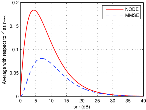
Figure 3: Comparison of the NODE with the MMSE in the continuous-time Gaussian channel of Example 1.

In Fig. 3, $\overline{\mathrm{node}}(\mathrm{snr})$ and $\overline{\mathrm{mmse}}(\mathrm{snr})$ are plotted against $10\log_{10}\mathrm{snr}$ for $\mathrm{snr}\geq 1$. Observe the difference in size.

References

- [1] D. Guo, S. Shamai (Shitz), and S. Verdú, “Mutual information and minimum mean-square error in Gaussian channels,” IEEE Trans. Inf. Theory, vol. 51, pp. 1261–1282, 2005.
- [2] E. Hammerich, “On the heat channel and its capacity,” in Proc. IEEE Int. Symp. Inf. Theory, Seoul, South Korea, 2009, pp. 1809–1813.
- [3] E. Hammerich, “On the capacity of the heat channel, waterfilling in the time-frequency plane, and a C-NODE relationship,” 2014 [Online]. Available: arXiv:1101.0287
- [4] D. O. North, Analysis of the factors which determine signal/noise discrimination in pulsed-carrier systems. Rept. PTR-6C, RCA Labs., Princeton, NJ, USA, 1943.
- [5] R. G. Gallager, Information Theory and Reliable Communication. New York, NY: Wiley, 1968.
- [6] E. Hammerich, “Waterfilling theorems for linear time-varying channels and related nonstationary sources,” IEEE Trans. Inf. Theory, vol. 62, pp. 6904–6916, 2016.
- [7] R. Bustin, M. Payaro, D. P. Palomar, and S. Shamai (Shitz), “On MMSE crossing properties and implications in parallel vector Gaussian channels,” IEEE Trans. Inf. Theory, vol. 59, pp. 818–844, 2013.
- [8] E. Hammerich, “Capacity and normalized optimal detection error in Gaussian channels,” 2017 [Online]. Available: arXiv:1701.05523