Abstract

This article provides a weighted model confidence set, whenever underling model has been misspecified and some part of support of random variable $X$ conveys some important information about underling true model. Application of such weighted model confidence set for local and mixture model confidence sets have been given. Two simulation studies have been conducted to show practical application of our findings.

Keywords: Inference Under Constraints; Kullback–Leibler Divergence; Model Confidence Set; Local Goodness of Fitness; Mixture Models.
2010 Mathematics Subject Classification: 62G07, 62F25, 62E17, 62F30, 62F03

1 Introduction

Approximating an unknown density function $h(\cdot)$ is an interesting problem which has a wide range of applications in statistical inference and data analysis. To find out an appropriate approximation, in first step, one has to collect a collection of family of distributions, say models, which can be appropriate (in some sense) competing for $h(\cdot).$ Then, in the second step, unknown parameters of such selected models have to be estimated using an appropriated (in some sense) estimation method. Such collection of appropriate competing models either belong to a family of distributions (say a class of nested models) or a collection $k(\geq 2)$ families of distributions (say a class of non-nested models). In the most statistical approaches using visual (such as qq–plots) or nonparametric (e.g. Kolmogorov–Smirnov test) tools, a nested models has been selected. Then, using an appropriate estimation method (such maximum likelihood, Bayesian, etc) unknown density $h(\cdot)$ has been approximated. But for the non-nested approach, selecting an appropriate non-nested models is a difficult task.

A considerable body of literature has been devoted to inference under a class of non-nested models. For instance: using the generalized likelihood ratio (${\cal LR}$) test, Cox (1961, 1962) developed a statistic test to compare two non-nested models. Atkinson (1970) considered a combined models as an appropriated competing for an unknown model. Then, he derived a statistical testing procedure to: (1) study departure from one model in the direction of another and (2) test the hypothesis that all fitted models are equivalent. Pesaran (1974) employed the Cox’s test (developed for comparing separate families of hypotheses) to study the choice between two non-nested linear single-equation econometric models. Pesaran & Deaton (1978) extended Pesaran (1974)’s findings to cover multivariate nonlinear models whenever full information maximum likelihood estimation is available. Davidson & MaKinnson (1981, 2002) considered several popular procedures which test an econometric model and they established those procedures are closely related, but not identical, to the non-nested hypothesis tests which was proposed by Pesaran & Deaton (1978). Pesaran (1987) emphasized the distinction between a “local null” and a “local alternative”. Then, under local alternatives, they derived the asymptotic distribution of the Cox’s test statistic. Fisher & McAleer (1981) derived two modified ${\cal LR}$ tests that are asymptotically equivalent to the Cox’s test. Dastoor (1983) studied different between Cox’s and Atkinson’s statistics. In 1989, using concept of the Kullback–Leibler divergence, Vuong extended Cox’s test. The Vuong’s test compares two competing density functions based upon the expectation of their ${\cal LR}$ statistic. Based upon minimization of expectation of the Akaike Information Criteria (AIC), Shimodaira (1998) constructed a confidence set. Lo, et al. (2001) showed that under Vuong’s assumptions the ${\cal LR}$ statistic based upon the Kullback–Leibler divergence and random sample $X_{1},X_{2},\cdots,X_{n}$ for hypothesis test

${\cal H}_{0}:X_{i}\sim$ $k_{0}$-component normal mixture   v.s.  ${\cal H}_{1}:X_{i}\sim$ $k_{1}$-component normal mixture

is asymptotically distributed as a weighted sum of independent chi-squared random variables with one degree of freedom. Hansen, et al. (2003), via a simulation study, showed that the model confidence set captures the superior models across a range of significance levels. Lu, et al. (2008) compared the Wald’s and Cox’s statistics based upon a simulation study. They showed that the small sample behavior of both statistics is closed to their asymptotic distributions. Hansen, et al. (2011) employed confidence set approach to study density of inflation in a given data set and the best Taylor rule regression for an empirical problem. Sayyareh (2012) constructed a tracking interval for the problem of selecting an appropriate estimation of unknown density $h(\cdot)$ among a class of non-nested families of distributions whenever data arrived from a Type II right censored phenomena. Li, et al. (2012) provided a Bayesian approach to the problem of nonparametric estimation of unknown density $h(\cdot).$

Using the Kullback–Leibler (${\cal KL}$) divergence along with Vuong’s test, this article constructs a set of appropriate weighted models, say weighted model confidence set, for unknown true density $h(\cdot)$ which is a subset of a class of non-nested models. A weighted confidence set is a set of models that is constructed such that it will contain the best model with a given level of confidence. All models which take to the weighted model confidence set are equivalent in terms of closeness to true density $h(\cdot).$ Applications of such weighted model confidence set has been given for local and mixture goodness of fitness. Practical implementation of the results has been confirmed through two simulation studies.

The rest of this article developed as follows. Section 2 collects some pertinent concepts of the Kullback–Leibler divergence, likelihood ratio tests and some mathematical background for the problem. Main results have been explored in Section 3. Two simulation studies have been conducted in Section 4.

2 Preliminaries

The Kullback–Leibler divergence, say ${\cal KL},$ is widely employed statistic to select an appropriate model among a class of competing models. Suppose $\log\frac{h(X)}{f(X;\theta)}$ stands for the log–likelihood ratio for density function $f(\cdot)$ and unknown true density $h(\cdot)$, for an observation $X.$ The expectation of this ratio, with respect to true density $h(\cdot),$ is ${\cal KL}$ divergence between $f(\cdot)$ and $h(\cdot)$. In other words,

$${\cal KL}(h||f) = E_{h}\left\{\log\left(\frac{h(X)}{f(X;\theta)}\right)\right\}$$

$$= E_{h}\{\log h(X)\}-E_{h}\left\{\log f(X;\theta)\right\},$$

where $E_{h}\{\log h(X)\}$ and $E_{h}\left\{\log f(X;\theta)\right\}$ present irrelevant and relevant parts of ${\cal KL}$ divergence, respectively. The expectation $E_{h}\{\log f(X;\theta)\}$ plays a vital role in this article. The ${\cal KL}$ divergence is a nonnegative value which cannot be consider as a distance. But from its definition, one may conclude that ${\cal KL}(h||f)=0$ implies that $h(\cdot)=f(\cdot;\theta),$ for all $\theta\in\Theta.$ To select an appropriate set of models among a class of non-nested competing models, it suffices to consider just relevant part of the ${\cal KL}$ divergence.

The Hellinger and $L^{2}$ distances between two density functions $f$ and $g$ have been defined by

$$H(f;g) = \sqrt{\int_{\mathbb{R}}\left(\sqrt{f(x)}-\sqrt{g(x)}\right)^{2}dx};$$

$$L^{2}(f;g) = \sqrt{\int_{\mathbb{R}}(f(x)-g(x))^{2}dx}.$$ (1)

The Hellinger and $L^{2}$ are two symmetric and non-negative distances that satisfies the triangle inequality. Moreover, convergence in Kullback–Leibler divergence implies convergence of the Hellinger and $L^{2}$ distances, see Van Erven & Harremos (2014) for more details. On other hand, the Kullback–Leibler divergence has a probabilistic/statistical meaning while Hellinger and $L^{2}$ distances do not. Therefore, in model selection literature the Kullback–Leibler divergence is a well-known distance which measures information lost whenever $f$ is used to approximate $g,$ see Lv & Liu (2014) for more details.

Suppose $X_{1},X_{2},\cdots,X_{n}$ is a sequence of i.i.d. random variables with common and unknown density function $h(\cdot)$. Moreover, suppose that two competing classes of models

$${\cal F}_{\Theta} = \left\{f(\cdot;\theta):~{}\theta\in\Theta\subseteq{\mathbb{R}}^{p}\right\}$$

$${\cal G}_{\Gamma} = \left\{g(\cdot;\gamma):~{}\gamma\in\Gamma\subseteq{\mathbb{R}}^{q}\right\}$$

can be viewed as two appropriate approximations for $h(\cdot),$ where $\Theta$ and $\Gamma,$ respectively, represent two different parameter spaces with dimensions $p$ and $q$. Two classes of models ${\cal F}_{\Theta}$ and ${\cal G}_{\Gamma}$ are called two non-nested classes if and only if ${\cal F}_{\Theta}\cap{\cal G}_{\Gamma}=\emptyset.$ Note that, the model ${\cal G}_{\Gamma}$ is nested in ${\cal F}_{\Theta}$ if and only if ${\cal G}_{\Gamma}\subset{\cal F}_{\Theta}.$ The following represents formal definition of non-nested models which employs in model selection literature. The model ${\cal F}_{\Theta}$ with respect to $h(\cdot)$ is called well-specified if and only if there exists $\theta\in\Theta$ such that $h(\cdot)\equiv f(\cdot;\theta),$ Otherwise, model ${\cal F}_{\Theta}$ with respect to $h(\cdot)$ is misspecified.

The most popular criteria in model selection has been coined and developed by Fisher (1921, 1922). In his seminal work, he employed concept of the maximum likelihood estimation method to develop a selection method criteria, well-known as a maximum likelihood method. This article utilizes a more advanced version of the maximum likelihood method, well-known as a quasi maximum likelihood estimator, say QMLE, that will be used in the rest of this article. The following represents definition of the QMLE.

Definition 1.

Suppose $X_{1},X_{2},\cdots,X_{n}$ is a random sample with unknown density $h(\cdot).$ Moreover, suppose that weighted density function $f(x;\theta)$ is an appropriate (in some sense) approximation for $h(\cdot).$ An estimator

$${\widehat{\theta}}^{n}=\arg\sup_{{\theta}\in\Theta}\,\sum_{i=1}^{n}\log f(X_{i};\theta)$$

which is maximized log–likelihood of ${\cal L}^{f}_{n}(\theta)=\sum_{i=1}^{n}\log f(X_{i};\theta)\}$ is well-known as the QMLE for parameter $\theta.$ Moreover, an estimator

$$\theta^{\star}=\arg\,\max_{\theta\in\Theta}E_{h}\left\{\frac{1}{n}\,\,{\cal L}^{f}_{n}(\theta)\right\}.$$

which minimizes the $\cal KL$ divergence is called pseudo estimator for $\theta.$

It is well-known that the usual MLE coincides with the QMLE whenever the family ${\cal F}_{\Theta}$ is well-specified with respect to the $h(\cdot)$, see White (1982b) for more details. Huber (1976) showed that the QML estimator, ${\widehat{\theta}}^{n}$, is a consistent estimator for pseudo estimator $\theta^{\star}$ whenever ${\cal F}_{\Theta}$ is misspecified with respect to $h(\cdot)$.

Since $E_{h}\{\log h(X)\}$ is free of $\theta,$ therefore based upon random sample $X_{1},\cdots,X_{n},$ two approximations $f_{\theta}(\cdot)$ and $g_{\gamma}(\cdot)$ for $h(\cdot)$ can be compared through their relevant parts of $\cal KL$ divergence.

Now, we collect some useful lemmas relating to the empirical distributions and likelihood ratio statistics which are useful in representing the main results of this article. The following from Barmalzan & Payandeh Najafabadi (2012) provides an ML estimator for unknown density function $h(\cdot).$

Lemma 1.

(Barmalzan & Payandeh Najafabadi, 2012) Suppose $X_{1},\cdots,X_{n}$ is a sequence of i.i.d. random variables with common and unknown density function $h(\cdot).$ Moreover, suppose that for given constant $t$ random variable $Y_{i}(t)$ has been defined by $Y_{i}(t)=I(X_{i}\leq t)$ for $i=1,\cdots,n$. Then, $Y_{1}(t),\cdots,Y_{n}(t)$ are i.i.d. random variables with common Bernoulli distribution with unknown parameter $H(t)=P(X_{1}\leq t).$ Therefore,

i)

The ML estimator for $H(t)$ is

$$\widehat{H}(t)=\frac{1}{n}\sum_{i=1}^{n}Y_{i}(t)=\frac{1}{n}\sum_{i=1}^{n}I(X_{i}\leq t);$$

ii)

The ML estimator for $h(t),$ based upon sample $x_{1},\cdots,x_{n},$ is $\widehat{h}(x_{i})=1/n,$ for $i=1,\cdots,n;$

iii)

The ML estimator for $E_{h}\{\log w(X;\theta_{0})\,f(X;\theta_{1})\},$ based upon sample $x_{1},\cdots,x_{n},$ is

$$E_{\widehat{h}}\{\log f(X;{\widehat{\theta}^{n})}\} = \frac{1}{n}\sum_{i=1}^{n}\log f(x_{i};{\widehat{\theta}^{n}});$$

iv)

An estimator $E_{\widehat{h}}\{\log f(X;{\widehat{\theta}^{n}})$ is converged, in probability, to $E_{h}\{\log f(X;\theta)\}.$

Based upon a random sample $X_{1},\cdots,X_{n}$ from unknown true density $h(\cdot),$ the likelihood ratio statistic, ${\cal LR}$, for ${\cal F}_{\Theta}$ against ${\cal G}_{\Gamma}$ is denoted by ${\cal LR}_{n}({\widehat{\theta}}^{n},\,{\widehat{\gamma}}^{n})$ and defined by subtracting log–likelihood of two family of weighted models (3), i.e.,

$${\cal LR}_{n}({\widehat{\theta}}^{n},\,{\widehat{\gamma}}_{n}) = {\cal L}^{f}_{n}({\widehat{\theta}}^{n})-{\cal L}^{g}_{n}({\widehat{\gamma}}^{n}),$$

where $f\in{\cal F}_{\Theta}$ and $g\in{\cal G}_{\Gamma}.$

The following recalls some useful properties of ${\cal LR}_{n}({\widehat{\theta}}^{n},\,{\widehat{\gamma}}^{n}),$ proof may be found in White (1982a) and Vuong (1989).

Lemma 2.

Suppose $X_{1},\cdots,X_{n}$ be a random sample with common and unknown true density $h(\cdot).$ Then, the likelihood ratio statistic ${\cal LR}_{n}({\widehat{\theta}}^{n},\,{\widehat{\gamma}}^{n})$ has the following properties:

(i)

Under some mild conditions (White, 1982a) ${\cal LR}_{n}^{w}\,({\widehat{\theta}}^{n},\,{\widehat{\gamma}}^{n})/n$ converges, almost surly, to

$${E_{h}\left\{\log\,\frac{f(X;{{\theta}^{\star}})}{g(X;{{\gamma}^{\star}})}\right\}};$$

(ii)

If $f(\cdot;{\theta^{\star}})\neq g(\cdot;{\gamma^{\star}})$, then $n^{-\,1/2}\,{\cal LR}_{n}\,({\widehat{\theta}}^{n},\,{\widehat{\gamma}}^{n})-n^{\,1/2}B_{\star}$ converges, in law, to normal distribution $N(0,\,A^{2}_{\star}),$

where

$$A^{2}_{\star}=Var_{h}\left\{\log\,\frac{f(X;{{\theta}^{\star}})}{g(X;{{\gamma}^{\star}})}\right\},~{}~{}~{}\&~{}~{}B_{\star}=E_{h}\left\{\log\,\frac{f(X;{{\theta}^{\star}})}{g(X;{{\gamma}^{\star}})}\right\}$$

and its estimator is

$$\widehat{A}^{2}_{n}=\frac{1}{n}\,\sum_{i=1}^{n}\left\{\log\,\frac{f(X_{i};{{\widehat{\theta}}^{n}})}{g(X_{i};{{\widehat{\gamma}}^{n}})}\right\}^{2}-\left\{\frac{1}{n}\sum_{i=1}^{n}\log\,\frac{f(X_{i};{{\widehat{\theta}}^{n}})}{g(X_{i};{{\widehat{\gamma}}^{n}})}\right\}^{2}.$$

The following section provides a model confidence set for true density function based upon a collection of weighted non-nested models, say weighted model confidence set. Application of such weighted model confidence set for local and mixture confidence sets have been given in two subsections.

3 Weighted Model Confidence Set

In traditional model-fitting strategy whole of observations received equal weight. Inference based on naive use of whole of information may be erroneous, since information conveyed by some of the observations is less important (in some sense) than the information conveyed by others. On the other hand, in many applications, only some parts of the space of variables are of interest, so that it makes sense to focus our attention in those regions. Weighted distribution are ideally suited model for these phenomenons. The weight function can be determined (or selected) to either reflecting such facts or taking into account some related information.

Suppose $\delta(x;\theta_{0})$ is a nonnegative function with finite expectation. Then, weighted density function $f^{w}(x;\theta_{0},\theta),$ based on realization $x$ of random variable $X$ under density function $f(x;\theta_{1}),$ has been defined by

$$f^{w}(x;\theta_{0},\theta) = \frac{\delta(x;\theta_{0})}{E_{f}(\delta(X;\theta_{0}))}f(x,\theta)$$

$$= w(x;\theta_{0})f(x,\theta)$$

where $x\in{\mathbb{R}}.$ Since increasing number of unknown parameters contradict with the parsimony’s principle (Posada & Buckley, 2004) and artificially impact on the Kullback–Leibler divergence (Barmalzan & Sayyareh, 2010). Hereafter now, we just consider a situation that either $\theta_{0}$ is a given constant or $\theta_{0}=\theta.$ Therefore, we just have $f^{w}(x;\theta),$ where $\theta\in\Theta$ and $x\in{\mathbb{R}}.$

Fisher (1934) developed concept of weighted distribution. Rao (1965) pointed out that: in many situations the recorded observations cannot be considered as a random sample from the original distribution due to non-observability of some events, damage caused to original observations, etc. The length biased distribution (weighted distribution with $w(x;\theta_{0})=x/E_{h}(X)$) has been found various applications in biomedical areas such as early detection of a disease. breast cancer (Zelen & Feinleib, 1969), human families and wild-life population studies (Rao, 1965), cardiology study involving two phases (Cnaan, 1985).

Weighted model selection has not received much attention in the model selection literature. The most of existence researches have been done regarding to bayes factor (Larose & Dey, 1996, 1998), nested model selection (Cheung, 2005, Ingrassia, et al., 2014), weighted model selection criteria, such as weighted least-squares support vector machines (Cawley, 2006), some information criterion, such as BIC and ICL, for mixture models as a weighted model (Dang, et al., 2014).

Now, Suppose that there is a collection of $k$ competing weighted non-nested models which could be used to describe random sample $X=(X_{1},\cdots,X_{n})$ obtained under common and unknown density $h(\cdot).$

$${\cal F}^{w}_{\Theta(i)} = \left\{f^{w}(\cdot;\theta(i)):~{}\theta_{i}\in\Theta(i)\subseteq{\mathbb{R}}^{p(i)}\right\}$$ (3)

where $\Theta(i)$ is parameter space with dimensions $p(i)$ and $w(\cdot)$ is a nonnegative and given weight function. Moreover, suppose that $\cal U$ denotes a collection of $k(\geq 2)$ weighted non-nested family of models ${\cal F}^{w}_{\Theta(i)},$ for $i\in{\cal M}=\{1,2,\cdots,k\},$ i.e., ${\cal U}^{w}=\bigcup_{i\in{\cal M}}{\cal F}^{w}_{\Theta(i)}.$

In the traditional model selection, the Kullback–Leibler divergence, ${\cal KL},$ is equally penalized all support of random variable $X.$ Weighted version of the Kullback–Leibler divergence can be defined as

$${\cal KL}\,\{h(X)||f^{w}(X;\theta)\} = E_{h}\{\log h(X)\}-E_{h}\left\{\log f^{w}(X;\theta)\right\}.$$

Now using the relevant expectation $E_{h}(\log f^{w}(X;\theta))$ one may conclude that: The class of models ${\cal F}^{w}_{\Theta(i)}$ can be considered as an appropriate approximation for unknown density $h(\cdot)$ if and only if the null hypothesis ${\cal H}_{0i}$ in the following hypothesis test

$$\left\{{\begin{array}[]{*{20}c}{{\cal H}_{0i}:E_{h}\{\log f^{w}(X;{\theta^{\star}(i)})\}\geq max_{j\,\in{\cal M}\backslash\{i\}}\,E_{h}\{\log f^{w}(X;{\theta^{\star}(j)})\},}&{}\hfil&{}\hfil\\ {}\hfil&{}\hfil&{}\hfil\\ {{\cal H}_{1i}:E_{h}\{\log f^{w}(X;{\theta^{\star}(i)})\}<\ max_{j\,\in{\cal M}\backslash\{i\}}\,E_{h}\{\log f^{w}(X;{\theta^{\star}(j)})\},}&{}\hfil&{}\hfil\\ \end{array}}\right.$$ (7)

has been accepted at significance level $\alpha,$ where $\theta^{\star}(i)=\arg\,\max_{\theta\in\Theta(i)}E_{h}\{\frac{1}{n}\,\,{\cal L}^{f^{w}}_{n}(\theta(i))\}.$

The null hypothesis ${\cal H}_{0i}$, for $i\in{\cal M}=\{1,\cdots,n\}$ in hypothesis test (7), at significance level $\alpha,$ will be rejected in favor of ${\cal H}_{1i}$ if and only if

$$\left\{\min_{{j\,\in{\cal M}}\backslash\{i\}}\,T_{ij}<-z_{\frac{\alpha}{k-1}}\right\},$$

where

$$T_{ij}:=\frac{n^{-\,1/2}\left\{{\cal L}_{n}^{f^{w}}(\widehat{\theta}^{\star}(i))-{\cal L}_{n}^{f^{w}}(\widehat{\theta}^{\star}(j))-(\dim(\theta(i))-\dim(\theta(j)))\right\}}{{{\widehat{A}}_{n}}},$$

$\dim(\cdot)$ denotes dimension and $z_{p}$ is the $p^{\hbox{th}}$ quantile of standard normal distribution, and ${\cal L}^{f^{w}}$ stands for the log–likelihood based upon random sample $X_{1},\cdots,X_{n},$ i.e., ${\cal L}^{f^{w}}_{n}(\theta)=\sum_{i=1}^{n}\log\{w(X_{i};\theta)\,f(X_{i};\theta)\}.$ For more details about this hypothesis test in the non-nested models and its applications, interested readers may refer to Barmalzan & Payandeh Najafabadi (2012), among others.

To simplify the idea which behind of our weighted confidence set, consider a situation that we have only two competing weighted non-nested family of models ${\cal F}^{w}_{\Theta(1)}$ and ${\cal F}^{w}_{\Theta(2)}.$ One may setup following two hypothesis tests

$${\cal H}_{0}^{(1)}:E_{h}\{\log f^{w}(X;{\theta_{\star}(1)})\}\geq E_{h}\{\log f^{w}(X;{\theta_{\star}(2)})\} v.s. {\cal H}_{1}^{(1)}:E_{h}\{\log f^{w}(X;{\theta_{\star}(1)})\}<E_{h}\{\log f^{w}(X;{\theta_{\star}(2)})\};$$

$$and$$

$${\cal H}_{0}^{(2)}:E_{h}\{\log f^{w}(X;{\theta_{\star}(2)})\}\geq E_{h}\{\log f^{w}(X;{\theta_{\star}(1)})\} v.s. {\cal H}_{1}^{(2)}:E_{h}\{\log f^{w}(X;{\theta_{\star}(2)})\}<E_{h}\{\log f^{w}(X;{\theta_{\star}(1)})\}.$$

Suppose that ${\bf\tau}$ denotes a $100(1-\alpha)\%$ weighted model confidence set for $h(\cdot).$ Using the above two hypothesis tests, one may include ${\cal F}^{w}_{\Theta(1)}$ in ${\bf\tau}$ whenever ${\cal H}_{0}^{(1)}$ has been accepted at significance level $\alpha/(2-1)=\alpha.$ Similarly, one may include ${\cal F}^{w}_{\Theta(2)}$ or both ${\cal F}^{w}_{\Theta(1)},{\cal F}^{w}_{\Theta(2)}$ in ${\bf\tau}$ whenever ${\cal H}_{0}^{(2)}$ and ${\cal H}_{0}^{(1)}$, ${\cal H}_{0}^{(2)}$ has been accepted at significance level $\alpha,$ respectively. Therefore, the $100(1-\alpha)\%$ weighted model confidence set is one of these three sets ${\bf\tau}=\{{\cal F}^{w}_{\Theta(1)}\},$ ${\bf\tau}=\{{\cal F}^{w}_{\Theta(2)}\},$ or ${\bf\tau}=\{{\cal F}^{w}_{\Theta(1)};{\cal F}^{w}_{\Theta(2)}\}.$

The following theorem formalizes the above idea. Its proof is similar to Barmalzan & Payandeh Najafabadi (2012, Theorem 1).

Theorem 1.

Suppose $X_{1},X_{2},\cdots,X_{n}$ is a random sample with common and unknown density $h(\cdot).$ Moreover, suppose that $\cal U$ is a collection of $k(\geq 2)$ weighted non-nested family of models ${\cal F}^{w}_{\Theta(i)},$ for $i\in{\cal M}:=\{1,2,\cdots,k\}.$ Then, the $100(1-\alpha)\%$ weighted model confidence set for $h(\cdot)$ is given by

$$\tau^{w} = \displaystyle\cup_{i\in{\cal M}}\left\{{\cal F}^{w}_{\Theta(i)}:~{}{\cal F}^{w}_{\Theta(i)}\in{\cal U}^{w}~{}\&~{}\min_{{j\,\in{\cal M}}\backslash\{i\}}\,T_{ij}>c\right\},$$

where $c:=z_{\alpha/(k-1)}.$

Note that the above weighted model confidence set is not empty because it at least contains the maximum $E_{h}\{\log w(X;\theta)f(X;\theta)\}$ model with an error smaller than significance level $\alpha.$

Remark 1.

Suppose $X_{1},X_{2},\cdots,X_{n}$ is a random sample with common unknown true density $h(\cdot).$ Moreover, suppose $\cal U^{\omega}$ is a collection of $k(\geq 2)$ weighted non-nested models

$${\cal F}_{\Theta(i)}^{\omega} = \left\{f^{w}(\cdot;{\theta(i)}):=\frac{\delta(\cdot;\theta(i))}{E_{h}(\delta(X;\theta(i)))}f_{\theta(i)}(\cdot):~{}\theta(i)\in\Theta(i)\subseteq{\mathbb{R}}^{p(i)}\right\},~{}~{}i\in{\cal M}=\{1,2,\cdots,k\}.$$

Then, the $100(1-\alpha)\%$ weighted model confidence set for unknown true density $h(\cdot)$ is given by

$$\tau^{w} = \displaystyle\cup_{i\in{\cal M}}\left\{{\cal F}^{w}_{\Theta(i)}:~{}{\cal F}_{\Theta(i)}^{\omega}\in{\cal U}^{w}~{}\&~{}\min_{{j\,\in{\cal M}}\backslash\{i\}}\,T_{ij}^{\omega}>z_{\frac{\alpha}{k-1}}\right\},$$

where

$$T_{ij}^{\omega}:=\frac{n^{-\,1/2}\left\{{\cal L}_{n}^{f_{i}^{\omega}}(\widehat{\theta}^{\star}(i))-{\cal L}_{n}^{f_{j}^{\omega}}(\widehat{\theta}^{\star}(j))-(\dim(\theta(i))-\dim(\theta(j)))\right\}}{{{\widehat{A}}_{n}^{\omega}}}.$$

The weight function $w(\cdot;\theta)$ selects based upon nature of problem in the hand or local goodness of fitness. The above idea may also develop to mixture model selection.

3.1 Application to local Model Confidence Set

In practical situations, sometimes different parts of the data (or support of random variable $X$) may be weighted differently. This local consideration is perfectly reasonable, because it provides lower variance for observations and consequently more information, see Hand & Vinciotti (2003) for more details. On the other hand, in many practical problems all parts of the distributions are not conveyed of equal information about under study phenomenon. In the situation where the true model is properly specified, this fact is not a big issue since under these circumstances a good fit in some region will not lead a poor fit in another region. However, the problem arrives whenever model is misspecified that a good fit in some region may well reduce from quality of fit in another region. Improving the fit of a misspecified model in some specified part of the space by forcing a close fit between the model and the underlying distributions in that region may be achieved through differential weighting. Note, however, that the choice of weights ignores the fact that different points may be of differing degree of importance in the context of the problem.

Using result of Theorem 1, the following provides a local model confidence set.

Remark 2.

Suppose $X_{1},X_{2},\cdots,X_{n}$ is a random sample with common and unknown true density $h(\cdot).$ Moreover, suppose that $A$ is a subset of support $X$ where conveys some important information. Then, the $100(1-\alpha)\%$ model confidence set in subset $A,$ say local model confidence set, is given by:

$$\displaystyle\tau^{w} = \displaystyle\bigcup_{i\in{\cal M}}\left\{{\cal F}_{\Theta(i)}^{w}:~{}{\cal F}_{\Theta(i)}^{w}\in{\cal U}^{w}~{}\&~{}\min_{{j\,\in{\cal M}}\backslash\{i\}}\,T_{ij}^{w}>z_{\frac{\alpha}{k-1}}\right\}.$$

where ${\cal U}^{w}$ is a collections of $k(\geq 2)$ weighted non-nested models, $w(x)=I_{A}(x)/P_{h}(X\in A),$ and $I_{A}(\cdot)$ stands for the indicator function.

It is worthwhile mentioning that the above set $\tau^{w}$ provides a $100(1-\alpha)\%$ confidence set for true density $h(\cdot)$ just on subset $A\subset{\mathbb{R}}$ not for whole of support $X.$

3.2 Application to Mixture Model Confidence Set

Using weighted model confidence set, one may go beyond of regular and classical model confidence set and consider mixture model confidence set. Such $100(1-\alpha)\%$ mixture confidence set can be obtained by the following three steps:

Step 1:

Partition whole of support of random variable $X$ into $m$ partitions;

Step 2:

Construct a $100(1-\beta)\%,$ where $0<\beta\leq 1-(1-\alpha)^{1/m},$ local confidence set for each partition;

Step 3:

Estimate an optimal mixture weight using a different criteria.

Step 3 provides an optimal $100(1-\alpha)\%$ mixture confidence set from another optimal criteria.

The following theorem illustrates the above three steps whenever support of random variable $X$ partitions into two disjoint sets $A$ and $A^{\prime},$ i.e., $A\cup{A^{\prime}}={\mathbb{R}}$ and $A\cap{A^{\prime}}=\varnothing.$

Theorem 2.

Suppose $X_{1},X_{2},\cdots,X_{n}$ is a random sample with common and unknown true density $h(\cdot)$ and ${\cal U}^{w_{1}}$ and ${\cal W}^{w_{2}}$ are two collections of $k_{1}(\geq 2)$ and $k_{2}(\geq 2)$ non-nested models, respectively, which locally appropriated for $h(\cdot).$ Moreover, suppose that

$$\displaystyle\tau^{w_{1}} = \displaystyle\bigcup_{i\in{\cal M}_{1}}\left\{{\cal F}_{\Theta(i)}^{w_{1}}:~{}{\cal F}_{\Theta(i)}^{w_{1}}\in{\cal U}^{w_{1}}~{}\&~{}\min_{{j\,\in{\cal M}_{1}}\backslash\{i\}}\,T_{ij}^{w_{1}}>z_{\frac{\beta}{k_{1}-1}}\right\};\qquad{\cal{M}}_{1}\in\{1,2,\cdots,k_{1}\}$$

$$\displaystyle\tau^{\omega_{2}} = \displaystyle\bigcup_{i\in{\cal M}_{1}}\left\{{\cal G}_{\Gamma(i)}^{w_{2}}:~{}{\cal G}_{\Gamma(i)}^{w_{2}}\in{\cal W}^{w_{2}}~{}\&~{}\min_{{j\,\in{\cal M}_{2}}\backslash\{i\}}\,T_{ij}^{w_{2}}>z_{\frac{\beta}{k_{2}-1}}\right\};\qquad{\cal{M}}_{2}\in\{1,2,\cdots,k_{2}\}$$

are two $100(1-\beta)\%$ local model confidence set for unknown density $h(\cdot)$ where $0<\beta<1-\sqrt{1-\alpha}.$ Then, an optimal $100(1-\alpha)\%$ global model confidence set for unknown density $h(\cdot)$ which minimized ${\cal KL}$ distance between convex combination of elements of $\tau^{w_{1}}$ and $\tau^{w_{2}}$ and $h(\cdot)$ is given by

$$\tau = \displaystyle\bigcup_{(i,j)\in{\cal M}_{1}\times{\cal M}_{2}}\left\{\alpha^{opt}_{ij}{f}^{w_{1}}(x;{{\hat{\theta}}(i)})+(1-\alpha^{opt}_{ij}){g}^{w_{2}}(x;{{\hat{\gamma}}(j)}):~{}~{}{f}^{w_{1}}(x;{{\hat{\theta}}(i)})\in\tau^{w_{1}}~{}\&~{}{g}^{w_{2}}(x;{{\hat{\gamma}}(j)})\in\tau^{w_{2}}\right\},$$

where $w_{1}(x)=I_{A}(x)/P_{h}(X\in A)$ and $w_{2}(x)=I_{A^{\prime}}(x)/P_{h}(X\in{A^{\prime}})$ are two given weight functions in two partitions $A$ and ${A^{\prime}}$ (where $A\cup{A^{\prime}}={\mathbb{R}}$ and $A\cap{A^{\prime}}=\varnothing$),

$$\displaystyle\alpha^{opt}_{ij} = \min\{1,~{}\max\{0,~{}argmax\{{\hat{\Psi}}(\alpha_{ij})\}\}\},$$ (8)

and ${\hat{\Psi}}(\alpha_{ij})=\sum_{l=1}^{n}\left(\log(\alpha_{ij}{f}^{w_{1}}(x_{l};{{\hat{\theta}}(i)})+(1-\alpha_{ij}){g}^{w_{2}}(x_{l};{{\hat{\gamma}}(j)}))\right)/n.$

Proof. Suppose $f(\cdot):=\alpha_{ij}{f}^{w_{1}}(\cdot;{{\hat{\theta}}(i)})+(1-\alpha_{ij}){g}^{w_{2}}(\cdot;{{\hat{\gamma}}(j)})$ is a member of $\tau.$ Therefore,

$$P(f\in\tau) = P\left(\alpha_{ij}{f}^{w_{1}}(x;{{\hat{\theta}}(i)})+(1-\alpha_{ij}){g}^{w_{2}}(x;{{\hat{\gamma}}(j)})\in\tau\right)$$

$$= P\left({f}^{w_{1}}(x;{{\hat{\theta}}(i)})\in\tau^{w_{1}}\,and\,{g}^{w_{2}}(x;{{\hat{\gamma}}(j)})\in\tau^{w_{2}}\right)$$

$$= P\left({f}^{w_{1}}(x;{{\hat{\theta}}(i)})\in\tau^{w_{1}}\right)\,P\left({g}^{w_{2}}(x;{{\hat{\gamma}}(j)})\in\tau^{w_{2}}\right)$$

$$= P\left(\min_{{j\,\in{\cal M}_{1}}\backslash\{i\}}\,T_{ij}^{w_{1}}>z_{\frac{\beta}{k_{1}-1}}\right)\,P\left(\min_{{j\,\in{\cal M}_{2}}\backslash\{i\}}\,T_{ij}^{w_{2}}>z_{\frac{\beta}{k_{2}-1}}\right)$$

$$\geq (1-\beta)\,(1-\beta)$$

$$\geq 1-\alpha.$$

On the other hand, $f(\cdot)$ is a convex combination of elements of $\tau^{w_{1}}$ and $\tau^{w_{2}}.$ Now observe that the ${\cal KL}$ distance between $f(\cdot)$ and $h(\cdot)$ minimized if and only if

$$\Psi(\alpha_{ij}) = E_{h}\left(\log(\alpha_{ij}{f}^{w_{1}}(X;{{\hat{\theta}}(i)})+(1-\alpha_{ij}){g}^{w_{2}}(X;_{{\hat{\gamma}}(j)}))\right)$$

has been maximized in $\alpha_{ij}.$ The desired proof arrived from the fact that $\partial^{2}\Psi(\alpha_{ij})/\partial\alpha_{ij}^{2}\geq 0$ and ${\hat{\Psi}}(\cdot)$ is an estimator for $\Psi(\cdot).$ $\square$

4 Simulation Study

This section through two simulation studies shows that how one may employ the above findings in practical applications.

Example 1.

Suppose random sample $x_{1},x_{2},\cdots,x_{n}$ (for $n=50,200,300$) have been generated from a length biased (i.e., $w(x)=x/x/E_{h}(X)$) Lognormal model with parameters $\theta=(\mu=2,\sigma^{2}=0.5)$. For this simulation, we consider the following three length biased non-nested models.

$${\cal F}_{\Theta(1)} = \left\{f(x;{\theta(1)})=\frac{x}{exp\{\mu+\frac{1}{2}\sigma^{2}\}}.\,\frac{1}{x\,\sqrt{2\pi\sigma^{2}}}\,\exp\left\{-\frac{\left(\log x-\mu\right)^{2}}{2\sigma^{2}}\right\};\quad\theta(1)=(\mu,\sigma^{2})\right\};$$

$${\cal F}_{\Theta(2)} = \left\{f(x;{\theta(2)})=\frac{x}{\alpha\,\lambda}.\,\frac{1}{\lambda^{\alpha}\,\Gamma(\alpha)}\,x^{\alpha-1}\,\exp\left\{-\frac{x}{\lambda}\right\};\quad\theta(2)=(\alpha,\,\lambda)\right\};~{}\hbox{and}$$

$${\cal F}_{\Theta(3)} = \left\{f(x;{\theta(3)})=\frac{x}{\gamma\,\Gamma(1+\frac{1}{\beta})}.\,\frac{\beta}{\gamma}\,\left(\frac{x}{\gamma}\right)^{\beta-1}\,\exp\left\{-\left(\frac{x}{\gamma}\right)^{\beta}\right\};\quad\theta(3)=(\beta,\,\gamma)\right\}.$$

as a possible competing models to determine the underling density $h(\cdot).$

To obtain a $95\%$ confidence set for the true density function Lognormal $(2,0.5),$ using the Monte-Carlo method with the R software, we generate, 1000 times, three sample size with length $n=50,200,300$ from underling Lognormal model. Using such generated data along with the above three non-nested models, to build up a $95\%$ confidence set for true model $h(\cdot),$ one has to conduct the following hypothesis test at significance level $\alpha=0.05.$

$${\cal H}_{01}:E_{h}\{\log f(X;{\hat{\theta}(1)})\} \geq \max_{j\in\{2,\,3\}}\,E_{h}\{\log f(X;{\hat{\theta}(j)})\}~{}\hbox{v.s.}~{}{\cal H}_{11}:Reject~{}{\cal H}_{01};$$

$${\cal H}_{02}:E_{h}\{\log f(X;{\hat{\theta}(2)})\} \geq \max_{j\in\{1,\,3\}}\,E_{h}\{\log f(X;{\hat{\theta}(j)})\}~{}\hbox{v.s.}~{}{\cal H}_{12}::Reject~{}{\cal H}_{02};$$ (9)

$${\cal H}_{03}:E_{h}\{\log f(X;{\hat{\theta}(3)})\} \geq \max_{j\in\{1,\,2\}}\,E_{h}\{\log f(X;{\hat{\theta}(j)})\}~{}\hbox{v.s.}~{}{\cal H}_{13}::Reject~{}{\cal H}_{03}.$$

Table 1 shows decision of the above hypothesis tests at significance level $\alpha=0.05$ for sample size $n=50,200,300.$

Table 1: Results of the above hypothesis tests at level $\alpha=0.05.$ Hypothesis Test ${\cal H}_{01}$ v.s. ${\cal H}_{11}$ ${\cal H}_{02}$ v.s. ${\cal H}_{12}$ ${\cal H}_{03}$ v.s. ${\cal H}_{13}$ Sample Size Test Statistic Conclusion Test Statistic Conclusion Test Statistic Conclusion $n=50$ 0.98 ${\cal H}_{01}$ is accepted - 1.12 ${\cal H}_{02}$ is accepted - 1.48 ${\cal H}_{03}$ accepted $n=200$ 1.87 ${\cal H}_{01}$ is accepted - 1.88 ${\cal H}_{02}$ is accepted - 2.37 ${\cal H}_{03}$ is rejected $n=300$ 2.24 ${\cal H}_{01}$ is accepted - 2.24 ${\cal H}_{02}$ is rejected - 2.80 ${\cal H}_{03}$ is rejected

Using results of Table 1, the following $95\%$ confidence set for the true density function Lognormal $(2,0.5)$ has been given in Table 2.

Table 2: A $95\%$ confidence set for different sample size
Sample size A $95\%$ confidence set $n=50$ $\tau=\left\{{\cal F}_{\Theta(1)};\,{\cal F}_{\Theta(2)};\,{\cal F}_{\Theta(3)}\right\}$ $n=200$ $\tau=\left\{{\cal F}_{\Theta(1)};\,{\cal F}_{\Theta(2)}\right\}$ $n=300$ $\tau=\left\{{\cal F}_{\Theta(1)}\right\}$

The $95\%$ confidence set, given by Table 2, shows that the method works properly and the true model (Lognormal) falls in confidence set. For the interpretation of equivalence of the above confidence sets, see Sayyareh, et al. (2011).

The following example explores a situation where one single confidence set cannot consider as an appropriate model confidence set for true density function.

Example 2.

Suppose random sample $x_{1},x_{2},\cdots,x_{1000}$ have been generated from a following density function.

$$h(x)=\frac{1}{3}\,\frac{1}{0.5}\,e^{-|x+4|/0.5}+\frac{2}{3}\,\frac{e^{-(x-6)}}{(1+e^{-(x-6)})^{2}},\qquad x\in{\mathbb{R}}.$$ (10)

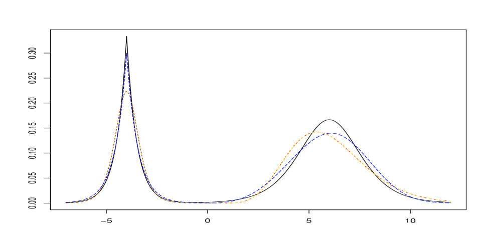
A histogram and true density function have been illustrated in part (a) of Figure 1.

From illustrated histogram, one may readily conclude that the underling distribution $h(\cdot)$ is a continuous distribution with two different modes. Thus, we cannot apply only one single density on the support $X$. In this case, in the first step, we divide whole of support into two partitions $A=(-\infty,0]$ and $A^{\prime}=(0,+\infty)$. Based upon graphical investigation, for the first part, we consider the non-nested competing models: {normal, cauchy, Logistic and Laplace} models and for the second part we propose three non-nested competing models: {gamma, Weibull and lognormal} models. Now in the following three steps, we develop a $95\%$ mixture confidence set for such generated observation.

Step 2-1: Local Confidence Set for A.

In this partition, we consider the following four non-nested models.

$${\cal F}^{w_{1}}_{\Theta(1)} = \left\{f^{w_{1}}(x;{\theta(1)})=w_{1}(x)\frac{1}{\sqrt{2\pi\sigma^{2}}}\,\exp\left\{-\frac{\left(x-\mu\right)^{2}}{2\sigma^{2}}\right\};\quad\theta(1)=(\mu,\sigma^{2}),\,x\in{\mathbb{R}}\right\};$$

$${\cal F}^{w_{1}}_{\Theta(2)} = \left\{f^{w_{1}}(x;{\theta(2)})=w_{1}(x)\frac{1}{\nu\pi\{1+(\frac{x-\theta}{\nu})^{2}\}};\quad\theta(2)=(\theta,\nu),\,x\in{\mathbb{R}}\right\};$$

$${\cal F}^{w_{1}}_{\Theta(3)} = \left\{f^{w_{1}}(x;{\theta(3)})=w_{1}(x)\frac{\frac{1}{\beta}\,e^{-(x-\gamma)/\beta}}{(1+e^{-(x-\gamma)/\beta})^{2}};\quad\theta(3)=(\gamma,\beta),\,x\in{\mathbb{R}}\right\};$$

$${\cal F}^{w_{1}}_{\Theta(4)} = \left\{f^{w_{1}}(x;{\theta(4)})=w_{1}(x)\frac{1}{b}\,e^{-|x-\lambda|/b};\quad\theta(4)=(\lambda,b),\,x\in{\mathbb{R}}\right\},$$

where $w_{1}(x)=I_{A}(x)/P_{h}(X\in A).$ To build up a $975\%$ confidence set for first part, one has to conduct the following hypothesis test at significance level $\beta=0.025.$

$${\cal H}^{f^{w_{1}}}_{01}:E_{h}\{\log f^{w_{1}}(X;{\hat{\theta}(1)})\} \geq \max_{j\in\{2,\,3,\,4\}}\,E_{h}\{\log f^{w_{1}}(X;{\hat{\theta}(j)})\}\quad~{}\hbox{v.s.}~{}\quad{\cal H}^{f^{w_{1}}}_{11}:Reject~{}{\cal H}^{f^{w_{1}}}_{01};$$

$${\cal H}^{f^{w_{1}}}_{02}:E_{h}\{\log f^{w_{1}}(X;{\hat{\theta}(2)})\} \geq \max_{j\in\{1,\,3,\,4\}}\,E_{h}\{\log f^{w_{1}}(X;{\hat{\theta}(j)})\}\quad~{}\hbox{v.s.}~{}\quad{\cal H}^{f^{w_{1}}}_{12}:Reject~{}{\cal H}^{f^{w_{1}}}_{02};$$

$${\cal H}^{f^{w_{1}}}_{03}:E_{h}\{\log f^{w_{1}}(X;{\hat{\theta}(3)})\} \geq \max_{j\in\{1,\,2,\,4\}}\,E_{h}\{\log f^{w_{1}}(X;{\hat{\theta}(j)})\}\quad~{}\hbox{v.s.}~{}\quad{\cal H}^{f^{w_{1}}}_{13}:Reject~{}{\cal H}^{f^{w_{1}}}_{03};$$

$${\cal H}^{f^{w_{1}}}_{04}:E_{h}\{\log f^{w_{1}}(X;{\hat{\theta}(4)})\} \geq \max_{j\in\{1,\,2,\,3\}}\,E_{h}\{\log f^{w_{1}}(X;{\hat{\theta}(j)})\}\quad~{}\hbox{v.s.}~{}\quad{\cal H}^{f^{w_{1}}}_{14}:Reject~{}{\cal H}^{f^{w_{1}}}_{04}.$$

Table 3 shows decision of the above hypothesis tests at significance level $\beta=0.025$ after 1000 irritations.

Table 3: Hypothesis tests at significant level $\beta=0.025$ for $A=(-\infty,0]$
Hypothesis Test Test Statistics Conclusion ${\cal H}^{f^{w_{1}}}_{01}$ v.s. ${\cal H}^{f^{w_{1}}}_{11}$ $-2.609$ ${\cal H}^{f^{w_{1}}}_{01}$ is rejected ${\cal H}^{f^{w_{1}}}_{02}$ v.s. ${\cal H}^{f^{w_{1}}}_{12}$ $-4.099$ ${\cal H}^{f^{w_{1}}}_{02}$ is rejected ${\cal H}^{f^{w_{1}}}_{03}$ v.s. ${\cal H}^{f^{w_{1}}}_{13}$ $-1.210$ ${\cal H}^{f^{w_{1}}}_{03}$ is accepted ${\cal H}^{f^{w_{1}}}_{04}$ v.s. ${\cal H}^{f^{w_{1}}}_{14}$ $0.0490$ ${\cal H}^{f^{w_{1}}}_{04}$ is accepted

Therefore, the desired a $975\%$ local confidence set for the first part is

$$\tau_{1}^{w_{1}}=\left\{{\cal F}^{w_{1}}_{\Theta(3)};{\cal F}^{w_{1}}_{\Theta(4)}\right\}.$$

Step 2-2: Local Confidence Set for $A^{\prime}$.

For the second part, we consider the following three non-nested competing models

$${\cal G}^{w_{2}}_{\Gamma(1)} = \left\{g^{w_{2}}(x;{\gamma(1)})=w_{2}(x)\frac{1}{\lambda^{\alpha}\,\Gamma(\alpha)}\,x^{\alpha-1}\,\exp\left\{-\frac{x}{\lambda}\right\};\quad\gamma(1)=(\alpha,\,\lambda),\,x\in{\mathbb{R}}^{+}\right\};$$

$${\cal G}^{w_{2}}_{\Gamma(2)} = \left\{g^{w_{2}}(x;{\gamma(2)})=w_{2}(x)\frac{\beta}{\gamma}\,\left(\frac{x}{\gamma}\right)^{\beta-1}\,\exp\left\{-\left(\frac{x}{\gamma}\right)^{\beta}\right\};\quad\gamma(2)=(\beta,\,\gamma),\,x\in{\mathbb{R}}^{+}\right\}$$

$${\cal G}^{w_{2}}_{\Gamma(3)} = \left\{g^{w_{2}}(x;{\gamma(3)})=w_{2}(x)\frac{1}{x\,\sqrt{2\pi\sigma^{2}}}\,\exp\left\{-\frac{\left(\log x-\mu\right)^{2}}{2\sigma^{2}}\right\};\quad\gamma(3)=(\mu,\sigma^{2}),\,x\in{\mathbb{R}}^{+}\right\},$$

where $w_{2}(x)=I_{A^{\prime}}(x)/P_{h}(X\in A^{\prime}).$ Using the above three competing models along with the following three hypothesis tests,

$${\cal H}^{g^{w_{2}}}_{01}:E_{h}\{\log g^{w_{2}}(X;{\hat{\gamma}(1)})\}\geq\max_{j\in\{2,\,3\}}\,E_{h}\{\log g^{w_{2}}(X;{\hat{\gamma}(j)})\}~{}\hbox{v.s.}~{}{\cal H}^{g^{w_{2}}}_{11}:Reject~{}{\cal H}^{g^{w_{2}}}_{01};$$

$${\cal H}^{g^{w_{2}}}_{02}:E_{h}\{\log g^{w_{2}}(X;{\hat{\gamma}(2)})\}\geq\max_{j\in\{1,\,3\}}\,E_{h}\{\log g^{w_{2}}(X;{\hat{\gamma}(j)})\}~{}\hbox{v.s.}~{}{\cal H}^{g^{w_{2}}}_{12}:Reject~{}{\cal H}^{g^{w_{2}}}_{02};$$

$${\cal H}^{g^{w_{2}}}_{03}:E_{h}\{\log g^{w_{2}}(X;{\hat{\gamma}(3)})\}\geq\max_{j\in\{1,\,2\}}\,E_{h}\{\log g^{w_{2}}(X;{\hat{\gamma}(j)})\}~{}\hbox{v.s.}~{}{\cal H}^{g^{w_{2}}}_{13}:Reject~{}{\cal H}^{g^{w_{2}}}_{03}.$$

Now, one may build up a $975\%$ model confidence set for the second part. Table 4 shows decision of the above hypothesis tests at significance level $\beta=0.025$ after 1000 irritations.

Table 4: Hypothesis tests at significant level $\beta=0.025$ for $A=(0,\infty)$
Hypothesis Test Test Statistics Conclusion ${\cal H}^{g^{w_{2}}}_{01}$ v.s. ${\cal H}^{g^{w_{2}}}_{11}$ $-1.540$ ${\cal H}^{g^{w_{2}}}_{01}$ is accepted ${\cal H}^{g^{w_{2}}}_{02}$ v.s. ${\cal H}^{g^{w_{2}}}_{12}$ $-1.520$ ${\cal H}^{g^{w_{2}}}_{02}$ is accepted ${\cal H}^{g^{w_{2}}}_{03}$ v.s. ${\cal H}^{g^{w_{2}}}_{13}$ $-3.360$ ${\cal H}^{g^{w_{2}}}_{03}$ is rejected

Therefore, the desired $975\%$ local confidence set for the second part is

$$\tau^{w_{2}}_{2}=\left\{{\cal G}^{w_{2}}_{\Gamma(1)};{\cal G}^{w_{2}}_{\Gamma(2)}\right\}.$$

Step 3: Mixture confidence set.

Now to construct a mixture $95\%$ model confidence set for unknown density function $h(\cdot),$ we minimized ${\cal KL}$ distance between convex combination of elements of $\tau^{w_{1}}_{1}$ and $\tau^{w_{2}}_{2}$ and $h(\cdot).$ Such convex combination is given by

$$\tau = \displaystyle\bigcup_{(i,j)\in\{3,4\}\times\{1,2\}}\left\{\alpha^{opt}_{ij}{f^{w_{1}}}(x;{{\hat{\theta}}(i)})+(1-\alpha^{opt}_{ij}){g^{w_{2}}}(x;{{\hat{\gamma}}(j)}):~{}~{}{f^{w_{1}}}(x;{{\hat{\theta}}(i)})\in\tau^{w_{1}}_{1}~{}\&~{}{g^{w_{2}}}(x;{{\hat{\gamma}}(j)})\in\tau^{w_{2}}_{2}\right\}.$$

Using result of Theorem (2), we estimate optimal mixture weight as $\alpha^{opt}_{31}=0.336$, $\alpha^{opt}_{32}=0.335$, $\alpha^{opt}_{41}=0.337$ and $\alpha^{opt}_{42}=0.335$. Table 5 represents the Hellinger and the $L^{2}$ distances for the $95\%$ mixture model confidence set.

Table 5: The values of Hellinger and $L^{2}$ distances for the $95\%$ mixture model confidence set
Combining Models Hellinger Distance $L^{2}$ Distance $\alpha^{opt}_{31}{f^{w_{1}}}(x;{{\hat{\theta}}(3)})+(1-\alpha^{opt}_{31}){g^{w_{2}}}(x;{{\hat{\gamma}}(1)})$ $0.0095$ $0.0052$ $\alpha^{opt}_{32}{f^{w_{1}}}(x;{{\hat{\theta}}(3)})+(1-\alpha^{opt}_{32}){g^{w_{2}}}(x;{{\hat{\gamma}}(2)})$ $0.0056$ $0.0035$ $\alpha^{opt}_{41}{f^{w_{1}}}(x;{{\hat{\theta}}(4)})+(1-\alpha^{opt}_{41}){g^{w_{2}}}(x;{{\hat{\gamma}}(1)})$ $0.0080$ $0.0037$ $\alpha^{opt}_{42}{f^{w_{1}}}(x;{{\hat{\theta}}(4)})+(1-\alpha^{opt}_{42}){g^{w_{2}}}(x;{{\hat{\gamma}}(2)})$ $0.0043$ $0.0022$

As Table 5 shows that all elements of the $95\%$ mixture model confidence set are appropriate choice for underling density function $h(\cdot),$ given by Equation (10).

Part (b) of Figure 1 illustrates element of the above $95\%$ mixture model confidence set and true density function. From this figure and Table 5, one may conclude that the above $95\%$ mixture model confidence set provides an appropriate approximation for true density function (10).

Figure 1: Part (a): Graphical illustration 1000 generated samples from true density function (10). Part (b): Graphical illustration of elements of the above $95\%$ mixture model confidence set and true density function.

5 Conclusion and Suggestions

This article considers the problem of constructing an appropriate model confidence set, whenever underling model has been misspecified and some part of support of random variable $X$ conveys some important information above misspecified density function $h(\cdot).$ Using weighted density functions, this article constructs a weighted model confidence set for true density function $h(\cdot).$ Applications for such weighted model confidence set for local and mixture model confidence sets have been given. Through a simulation study, we have been seen that the weighted model confidence set offers a convenient model confidence set for complex data. Our findings cannot practically employ whenever non-nested competing model contain a large number models. Therefore, we suggest to develop an one single procedure to built up such confidence model set.

References

- [1] Atkinson, A. C. (1970). A method for discriminating between models. Journal of the Royal Statistical Society, 32, 323–344.
- [2] Barmalzan, G. & Payandeh Najafabadi (2012). Model Confidence Set Based on Kullback-Leibler Divergence Distance. J. Statist. Res. Iran, 9, 115–129.
- [3] Barmalzan, G. & Sayyareh, A. (2010). The Choice of an Admissible Set of k Non-nested Models. Journal of Statistical Sciences, 4(2), 149–165.
- [4] Cawley, G. C. (2006). Leave-one-out cross-validation based model selection criteria for weighted LS-SVMs. IEEE, International Joint Conference on In Neural Networks. 1661–1668.
- [5] Cheung, Y. M. (2005). Maximum weighted likelihood via rival penalized EM for density mixture clustering with automatic model selection. IEEE Transactions on Knowledge and Data Engineering, 17(6), 750–761.
- [6] Cnaan, A. (1985). Survival models with two phases and length biased sampling. Communications in Statistics-Theory and Methods, 14(4), 861–886.
- [7] Cox, D. R. (1961). Tests of separate families of hyphotesis. Proceedings of the Fourth Berkeley Symposium on Mathematical Statistics and Probability, 1, 105–123.
- [8] Cox, D. R. (1962). Further results on tests of separate families of hyphotesis. Journal of the Royal Statistical Society, 24, 406–424.
- [9] Dang, U. J., Punzo, A., McNicholas, P. D., Ingrassia, S., & Browne, R. P. (2014). Multivariate response and parsimony for Gaussian cluster-weighted models. arXiv preprint arXiv:1411.0560.
- [10] Dastoor, N, K. (1983). Some aspects of testing non-nested hyopthesis. Journal of Econometrica, 21, 213-228.
- [11] Davidson, R. & MacKinnon, J. G. (1981). Several tests for model specification in the presence of alternative hypotheses. Journal of Econometrica, 29, 213–228.
- [12] Davidson, R. & MacKinnon, J. G. (2002). Bootstrap J tests of non-nested linear regression models. Journal of Econometrics, 109, 167–193.
- [13] Fisher, R. A. (1921). On the “Probable Error” of a Coefficient of Correlation Deduced from a Small Sample. Metron, 1, 3–32.
- [14] Fisher, R. A. (1922). The goodness of fit of regression formulae, and the distribution of regression coefficients. Journal of the Royal Statistical Society, 85 597–612.
- [15] Fisher, R. A. (1934). The effect of methods of ascertainment upon the estimation of frequencies. Annals of eugenics, 6(1), 13–25.
- [16] Fisher, G. R & McAleer, M. (1981). Alternative procedures and associated tests of significance for non-nested hypotheses. Journal of Econometrics, 16, 103–119.
- [17] Hand, D. J., & Vinciotti, V. (2003). Local versus global models for classification problems: fitting models where it matters. The American Statistician, 57(2), 124–131.
- [18] Hansen, P. R., Lunde, A., & Nason, J. M. (2003). Choosing the Best Volatility Models: The Model Confidence Set Approach. Oxford Bulletin of Economics and Statistics, 65, 839–861.
- [19] Hansen, P. R., Lunde, A. & Nason, J. M. (2011). The Model Confidence Set. Econometrica, 79, 453–497.
- [20] Huber, P. J. , The behavior of maximum likelihood estimate under nonstandard conditions. Proc. Fifth Berkeley Symposium in Mathematical Statistics and Probability. Berkeley, University of California Press, pp. 221-223.
- [21] Ingrassia, S., Minotti, S. C., & Punzo, A. (2014). Model-based clustering via linear cluster-weighted models. Computational Statistics & Data Analysis, 71, 159–182.
- [22] Larose, D. T., & Dey, D. K. (1996). Weighted distributions viewed in the context of model selection: a Bayesian perspective. Test, 5(1), 227–246.
- [23] Larose, D. T., & Dey, D. K. (1998). Modeling publication bias using weighted distributions in a Bayesian framework. Computational statistics & data analysis, 26(3), 279–302.
- [24] Li, S., Silvapulle, M. J., Silvapulle, P. & Zhang. X. (2012). Bayesian Approaches to Nonparametric Estimation of Densities on the Unit Interval. Technical report, Department of Econometrics and Business Statistics, Monash University, Australia.
- [25] Lo, Y., Mendell, N. R., & Rubin, D. B. (2001). Testing the number of components in a normal mixture. Biometrika,, 88, 767–778.
- [26] Lu, M., Mizon, G. E., & Monfardini, C. (2008). Simulation Encompassing: Testing Non-nested Hypotheses. Oxford Bulletin of Economics and Statistics, 70, 781–806.
- [27] Lv, J., & Liu, J. S. (2014). Model selection principles in misspecified models. Journal of the Royal Statistical Society: Series B (Statistical Methodology), 76(1), 141–167.
- [28] Pesaran, M. H. (1974). On the general problem of model selection. The Review of Economic Studies, 41, 153–171.
- [29] Pesaran, M. H. (1987). Global and partial non-nested hypotheses and asymptotic local power. Econometric Theory, 3, 69–97.
- [30] Pesaran, M. H., & Deaton, A. S. (1978). Testing non-nested nonlinear regression models. Econometrica: Journal of the Econometric Society, 46, 677–694.
- [31] Posada, D., & Buckley, T. R. (2004). Model selection and model averaging in phylogenetics: advantages of Akaike information criterion and Bayesian approaches over likelihood ratio tests. Systematic biology, 53(5), 793–808.
- [32] Rao, C. R. (1965). On discrete distributions arising out of methods of ascertainment. Sankhy: The Indian Journal of Statistics, Series A, 27(2-4), 311–324
- [33] Sayyareh, A. (2012). Tracking interval for selecting between non-nested models: An investigation for Type II right censored data. Journal of Statistical Planning and Inference, 142, 3201–3208.
- [34] Sayyareh, A., Obeidi, R., & Bar-hen, A. (2011). Empirical comparison between some model selection criteria. Communications in Statistics-Simulation and Computation, 89, 72–86.
- [35] Shimodaira, H. (1988). An application of multiple comparison techniques to model selection. Annals of Institute of Statistical Mathematics, 50, 1–13.
- [36] Van Erven, T., & Harremos, P. (2014). Rényi divergence and Kullback–Leibler divergence. IEEE Transactions on Information Theory, 60(7), 3797–3820.
- [37] Vuong, Q. H. (1989). Likelihood ratio test for model selection and non-nested hypotheses. Econometrica, 57, 307–333.
- [38] White, H. (1982a). Regularity conditions for Cox’s test of non-nested hypotheses. Journal of Econometrics, 19, 301–318.
- [39] White, H. (1982b). Maximum likelihood estimation of mis-spesified models. Econometrica, 50, 1–26.
- [40] Zelen, M., & Feinleib, M. (1969). On the theory of screening for chronic diseases. Biometrika, 56(3), 601–614.