Floquet-Mode Solutions of
Space-Time Modulated Huygens’ Metasurfaces

Abstract

A rigorous Floquet mode analysis is proposed for a zero thickness space-time modulated Huygens’ metasurface to model and determine the strengths of the new harmonic components of the scattered fields. The proposed method is based on Generalized Sheet Transition Conditions (GSTCs) treating a metasurface as a spatial discontinuity. The metasurface is described in terms of Lorentzian electric and magnetic surface susceptibilities, $\chi_{\text{ee}}$ and $\chi_{\text{mm}}$, respectively, and its resonant frequencies are periodically modulated in both space and time. The unknown scattered fields are then expressed in terms of Floquet modes, which when used with the GSTCs, lead to a system of field matrix equations. The resulting set of linear equations are then solved numerically to determine the total scattered fields. Using a finite-difference time domain (FDTD) solver, the proposed method is validated and confirmed for several examples of modulation depths ($\Delta_{p}$) and frequencies ($\omega_{p}$). Finally, the computed steady-state scattered fields are Fourier propagated analytically, for visualization of refracted harmonics. The proposed method is simple and versatile and able to determine the steady-state response of a space-time modulated Huygen’s metasurface, for arbitrary modulation frequencies and depths.

I Introduction

Recently, there has been a strong growing interest in Huygen’s metasurfaces due to their impedance matching capabilities with free-space and their versatile applications in wavefront shaping [Elliptical_DMS][GeneralizedRefraction][meta3]. They are constructed using a 2-D array of electrically small Huygen’s sources, exhibiting perfect cancellation of backscattered fields, due to optimal interactions of their electric and magnetic dipolar moments [Kerker_Scattering]. Some efficient implementations of Huygens’ metasurfaces are based on all-dielectric resonators [Kivshar_Alldielectric][Elliptical_DMS][AllDieelctricMTMS] and orthogonally collocated small electric and magnetic dipoles [Grbic_Metasurfaces][HuygenBook_Eleftheriades].

While the majority of the work on metasurfaces has been focussed on static (linear time invariant) metasurfaces, there is also a growing interest in dynamic metasurfaces, where the constitutive parameters of the metasurface unit cells are controlled in real-time. An important class of such dynamic electromagnetic structures is space-time modulated metasurfaces, where their constitutive parameters are periodically modulated in both space and time, at comparable frequency scales to the input excitations. This leads to a complex interaction of the incident wavefronts with the metasurfaces resulting in exotic effects such as generation of new harmonic components and Lorentz non-reciprocity [STGradMetasurface][ShaltoutSTMetasurface]. Space-time modulated metasurfaces fall within the general framework of space-time modulated mediums [TamirST][OlinerST], which have found important applications in acousto-optical systems for spectrum analysis, parametric oscillators and amplifiers, for instance [Goodman_Fourier_Optics][Saleh_Teich_FP][TamirAcoustoDiffraction].

Consequently, a combination of the wave-shaping capabilities of Huygens’ metasurfaces with space-time modulation principles, is an interesting avenue to explore for advanced electromagnetic wave control, in both space and time. To investigate into the properties of space-time modulated Huygens’ metasurfaces, a finite-difference time-domain (FDTD) technique has recently been proposed to analyze a zero thickness model of Huygens’ metasurfaces [Smy_Metasurface_Linear][Stewart_Metasurface_STM], based on Generalized Sheet Transition Conditions (GSTCs) [KuesterGSTC]. In contrast to the other existing techniques for analyzing static metasurfaces in frequency domain [CalozFDTD][Caloz_MetaModelling], the FDTD analysis is naturally applicable to the problem of space-time modulated metasurfaces, considered herein.

While such numerical methods are useful to determine the time-evolution of scattered waves from space-time modulated metasurfaces for a given input wave, efficient determination of steady-state response of the metasurface is an equally important problem to solve. This issue is addressed in this work, whereby exploiting the periodic nature of the spatio-temporal perturbation on the metasurface, the scattered fields are expressed in terms of Floquet modes. The Huygens’ metasurface is modelled using surface susceptibilities following a physically motivated Lorentzian profile, whose resonant frequencies are parametrized to emulate a space-time modulation of the metasurface. Combined with GSTCs, the Floquet mode amplitudes are computed by solving a set of linear equations. The proposed method thus efficiently computes the steady-state response of a zero-thickness space-time modulated Huygens’ metasurface, consistent with the FDTD field solutions. Furthermore, integrating the proposed method with analytical Fourier methods [Goodman_Fourier_Optics], the propagation of scattered fields are conveniently visualized in free-space.

The paper is structured as follows. Section II describes the problem statement of this work, and develops the fields equations governing the scattering fields from a space-time modulated metasurface based on GSTCs and Lorentz surface susceptibilities. Section III presents the proposed method based on Floquet mode expansions, forming the set of linear equations to be solved numerically. Several results are then presented for both time-only and space-time modulated metasurfaces. Conclusions are provided in Sec. IV, and a brief summary of the FDTD method is provided in Appendix V, for the sake of self-consistency and completeness of the paper.

II Space-Time Modulated Metasurfaces

II-A Problem Statement

Metasurfaces are zero thickness electromagnetic structures that act as discontinuities in space. The exact zero thickness nature of electromagnetic structures was developed by Idemen in terms of Generalized Sheet Transition Conditions (GSTCs) [IdemenDiscont], which were later applied to metasurfaces [KuesterGSTC]. Consider a Huygens’ metasurface illustrated in Fig. 1, where the metasurface lies in the $x-y$ plane at $z=0$, with a wave incidence on the left, normal to the surface. The wave interacts with the metasurface and produces a transmitted and a reflected wave, along the forward and backward direction, respectively. This interaction of the metasurface with the electromagnetic waves is described by the GSTCs, using the transverse components of electric and magnetic surface polarizabilities $\mathbf{P}$ and $\mathbf{M}$, as [Metasurface_Synthesis_Caloz]

$$\hat{\mathbf{z}}\times\Delta\mathbf{H}(x,t)=\frac{d\mathbf{P}_{||}(x,t)}{dt}$$ (1a)

$$\Delta\mathbf{E}(x,t)\times\hat{\mathbf{z}}=\mu_{0}\frac{d\mathbf{M}_{||}(x,t)}{dt},$$ (1b)

where

$$\Delta\mathbf{E}=(\mathbf{E}_{t}-\mathbf{E}_{0}-\mathbf{E}_{r}),\quad\Delta\mathbf{H}=(\mathbf{H}_{t}-\mathbf{H}_{0}-\mathbf{H}_{r}).$$

The surface polarizabilities on the Huygens’ metasurface are related to the average fields around the metasurface and can be described in terms of scalar electric and magnetic surface susceptibilities $\chi_{\text{ee}}$ and $\chi_{\text{mm}}$, respectively, as.

$$\mathbf{\tilde{Q}}_{||}(\omega)=\tilde{\chi}_{\text{ee}}\mathbf{\tilde{E}}_{\text{av}}(\omega),$$ (2a)

$$\mathbf{\tilde{M}}_{||}(\omega)=\tilde{\chi}_{\text{mm}}\mathbf{\tilde{H}}_{\text{av}}(\omega),$$ (2b)

$$\text{where}~{}\mathbf{\tilde{E}}_{\text{av}}=\left[\frac{\mathbf{\tilde{E}}_{0}+\mathbf{\tilde{E}}_{t}+\mathbf{\tilde{E}}_{r}}{2}\right],~{}\mathbf{\tilde{H}}_{\text{av}}=\left[\frac{\mathbf{\tilde{H}}_{0}+\mathbf{\tilde{H}}_{t}+\mathbf{\tilde{H}}_{r}}{2}\right]$$

and $\mathbf{Q}=\mathbf{P}/\epsilon_{0}$ is the normalized electric polarizability.

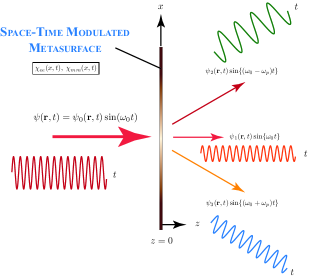
Figure 1: A general Illustration of a space-time modulated Huygens’ metasurface under normally incident CW plane-wave resulting in generation of several frequency harmonics, refracted along different angles. $\omega_{p}$ is the pumping frequency.

Next, consider a space-time modulated metasurface, whose electric and magnetic susceptibilities are both a function of space and time, i.e. $\chi_{\text{ee}}(x,t)$ and $\chi_{\text{mm}}(x,t)$. Let us restrict here to a periodic modulation only, with a pumping frequency $\omega_{p}$ and the spatial frequency $\beta_{p}$. Due to this periodic spatio-temporal perturbation on the metasurface, assumed to be infinite in size, the scattered transmission (and reflection) fields can be expressed in terms of Floquet series as

$$E_{t}(x,z=0_{+},t)=\sum_{n=0}^{\infty}q_{n}e^{j\omega_{n}t}e^{j\beta_{n}x},$$ (3)

where $\omega_{n}=\omega_{0}+n\omega_{p}$, and $\beta_{n}=\beta_{x0}+n\beta_{p}$ with $\beta_{x0}=0$ due to assumed normal input incidence. Each harmonic term of this expansion with a temporal frequency $\omega_{n}$, represents an oblique forward propagating plane-wave in the $+z$ direction, and making an angle $\theta_{n}$ measured from the normal of the metasurface, as illustrated in Fig. 1. These refraction angles are given by

$$\theta(\omega_{n})=\sin^{-1}\left[\frac{n}{(1+n\omega_{p}/\omega_{0})}\frac{\beta_{p}}{k_{0}}\right],$$ (4)

where $k_{0}$ is the free-space wavenumber of the fundamental frequency. Based on this simple physical argument, the angle of refraction of these newly generated frequency components from a space-time modulated metasurface, can be determined. However, the strengths of these harmonics (weights $q_{n}$) are still unknown and must be determined taking the exact electromagnetic interaction of the waves with the metasurface into account using the GSTCs of (1).

II-B Field Equations

The space-time modulated problem considered here is naturally treated in the time domain. Consequently, the surface susceptibilities must be defined in time domain as well. The most common, and causal, description of the susceptibilities is in terms of Lorentz dispersion, which is also typical of the Huygens’ sources used to construct the metasurfaces [Kivshar_Alldielectric][PDM_Gupta][Huygen_Microwave_Achouri]. Consequently, the electric and magnetic susceptiblities can be expressed as

$$\tilde{\chi}_{\text{ee}}(\omega)=\frac{\omega_{ep}^{2}}{(\omega_{e0}^{2}-\omega^{2})+i\alpha_{e}\omega}$$ (5a)

$$\tilde{\chi}_{\text{mm}}(\omega)=\frac{\omega_{mp}^{2}}{(\omega_{m0}^{2}-\omega^{2})+i\alpha_{m}\omega},$$ (5b)

where $(\omega_{e0}$, $\omega_{m0}),\;(\omega_{ep}$, $\omega_{mp}),\;(\alpha_{e},\alpha_{m})$ are the electric and magnetic resonant frequencies, plasma frequencies and loss coefficients, respectively.

The space-time modulation can now be introduced into the metasurface, by sinusoidally modulating, for instance, the resonant frequencies of the two Lorentzian susceptibilities, as [Stewart_Metasurface_STM]

$$\omega_{e0}(x,t)=\omega_{e0}\{1+\Delta_{e}\cos(\omega_{p}t+\beta_{p}x)\}$$ (6a)

$$\omega_{m0}(x,t)=\omega_{m0}\{1+\Delta_{m}\cos(\omega_{p}t+\beta_{p}x)\},$$ (6b)

where $\Delta_{e}$ and $\Delta_{m}$ are the modulation depths and the spatial frequencies of the perturbation, for electric and magnetic resonances, respectively. They can now be inserted into the GSTCs of (1), for a prescribed input fields, to determine the total scattered fields.

To illustrate the procedure, let us assume a normally incident plane-wave ($|\mathbf{E_{0}}|=\text{const.}$) where the corresponding transmitted and reflected fields, given by

$$\mathbf{E}_{0}(z,t)=E_{0}e^{j(\omega_{0}t-k_{0}z)}~{}\mathbf{\hat{y}},~{}\mathbf{H}_{0}(z,t)=\frac{\mathbf{\hat{z}}\times\mathbf{E}_{0}(z,t)}{\eta_{0}}$$ (7)

$$\mathbf{E}_{t}(z,t)=E_{t}(x,t)e^{-jk_{0}z}~{}\mathbf{\hat{y}},~{}\mathbf{H}_{t}(z,t)=\frac{\mathbf{\hat{z}}\times\mathbf{E}_{t}(z,t)}{\eta_{0}}$$

$$\mathbf{E}_{r}(z,t)=E_{r}(x,t)e^{+jk_{0}z}~{}\mathbf{\hat{y}},~{}\mathbf{H}_{r}(z,t)=\frac{\mathbf{E}_{r}(z,t)\times\mathbf{\hat{z}}}{\eta_{0}}.$$

Each of these field components are related to their respective polarizabilities on the metasurface (at $z=0$) through the Lorentz susceptibilities of (5) with (6), which can then be expressed in the time domain as [Smy_Metasurface_Linear]

$$\frac{d^{2}Q_{i}}{dt^{2}}+\omega_{e0}^{2}\{1+\Delta_{e}\cos(\omega_{p}t+\beta_{p}x)\}^{2}Q_{i}=\omega_{ep}^{2}E_{i}(t)$$ (8a)

$$\frac{d^{2}M_{i}}{dt^{2}}+\omega_{m0}^{2}\{1+\Delta_{m}\cos(\omega_{p}t+\beta_{p}x)\}^{2}M_{i}=\frac{\omega_{ep}^{2}}{\eta_{0}}E_{i}(t),$$ (8b)

where the subscript $i=0,t,r$ for incident, transmitted and reflected fields, respectively. Finally, all the scattered fields are related to their polarizabilities following the GSTCs of (1), as

$$\frac{dQ_{0}}{dt}+\frac{dQ_{t}}{dt}+\frac{dQ_{r}}{dt}=\frac{2}{\eta_{0}\epsilon_{0}}(E_{0}-E_{r}-E_{t}),$$ (9a)

$$\frac{dM_{0}}{dt}+\frac{dM_{t}}{dt}+\frac{dM_{r}}{dt}=\frac{2}{\mu_{0}}(E_{t}-E_{r}-E_{0})$$ (9b)

Equations (8) and (9) thus represent two sets of field equations, that must be solved to determine the transmitted and reflected fields, $E_{t}(x,z,t)$ and $E_{r}(x,z,t)$, in steady state, for a given input excitation $\mathbf{E_{0}}=E_{0}e^{j\omega_{0}t}~{}\mathbf{\hat{y}}$ at the input of the metasurface at $z=0_{-}$.

$$\sum_{n}\left[\Delta_{e1}a_{n-2}+\Delta_{e2}a_{n-1}+A_{e,n}a_{n}+\Delta_{e2}a_{n+1}+\Delta_{e1}a_{n+2}\right]e^{jn\Omega t}=E_{0}~{}\quad\text{(Incident E-Fields)}$$ (10)

$$\sum_{n}\left[\Delta_{e1}b_{n-2}+\Delta_{e2}b_{n-1}+A_{e,n}b_{n}+\Delta_{e2}b_{n+1}+\Delta_{e1}b_{n+2}-q_{n}\right]e^{jn\Omega t}=0~{}\quad\text{(Transmitted E-Fields)}$$

$$\sum_{n}\left[\Delta_{e1}c_{n-2}+\Delta_{e2}c_{n-1}+A_{e,n}c_{n}+\Delta_{e2}c_{n+1}+\Delta_{e1}c_{n+2}-p_{n}\right]e^{jn\Omega t}=0~{}\quad\text{(Reflected E-Fields)}$$

$$\sum_{n}\left[\Delta_{m1}d_{n-2}+\Delta_{m2}d_{n-1}+A_{m,n}d_{n}+\Delta_{m2}d_{n+1}+\Delta_{m1}d_{n+2}\right]e^{jn\Omega t}=-\frac{E_{0}}{\eta_{0}}~{}\quad\text{(Incident H-Fields)}$$

$$\sum_{n}\left[\Delta_{m1}e_{n-2}+\Delta_{m2}e_{n-1}+A_{m,n}e_{n}+\Delta_{m2}e_{n+1}+\Delta_{m1}e_{n+2}-b_{n}\right]e^{jn\Omega t}=0~{}\quad\text{(Transmitted H-Fields)}$$

$$\sum_{n}\left[\Delta_{m1}f_{n-2}+\Delta_{m2}f_{n-1}+A_{m,n}f_{n}+\Delta_{m2}f_{n+1}+\Delta_{m1}f_{n+2}-f_{n}\right]e^{jn\Omega t}=0~{}\quad\text{(Reflected H-Fields)}$$

$$\sum_{n}\left[2cB_{n}a_{n}+2cB_{n}b_{n}+2cB_{n}c_{n}+p_{n}+q_{n}\right]e^{jn\Omega t}=E_{0}~{}\quad\text{(GSTC Equation)}$$

$$\sum_{n}\left[\frac{\mu_{0}B_{n}}{2}d_{n}+\frac{\mu_{0}B_{n}}{2}e_{n}+\frac{\mu_{0}B_{n}}{2}f_{n}+p_{n}-q_{n}\right]e^{jn\Omega t}=-E_{0}~{}\quad\text{(GSTC Equation)}$$

 

$$\overbrace{\left[\begin{array}[]{cccc cccc}\mathbf{S_{e}}&0&0&0&0&0&0&0\\ 0&\mathbf{S_{e}}&0&0&0&0&0&-\mathbf{I}\\ 0&0&\mathbf{S_{e}}&0&0&0&-\mathbf{I}&0\\ 0&0&0&\mathbf{S_{m}}&0&0&0&0\\ 0&0&0&0&\mathbf{S_{m}}&0&0&\mathbf{I}/\eta_{0}\\ 0&0&0&0&0&\mathbf{S_{m}}&-\mathbf{I}/\eta_{0}&0\\ \mathbf{S_{g}}/(2c_{0})&\mathbf{S_{g}}/(2c_{0})&\mathbf{S_{g}}/(2c_{0})&0&0&0&\mathbf{I}&\mathbf{I}\\ 0&0&0&\mathbf{S_{g}}&\mathbf{S_{g}}&\mathbf{S_{g}}&\mathbf{I}&-\mathbf{I}\end{array}\right]}^{\mathbf{C_{n}}}\overbrace{\left[\begin{array}[]{c}\mathbf{a_{n}}\\ \mathbf{b_{n}}\\ \mathbf{c_{n}}\\ \mathbf{d_{n}}\\ \mathbf{e_{n}}\\ \mathbf{f_{n}}\\ \mathbf{p_{n}}\\ \mathbf{q_{n}}\end{array}\right]}^{\mathbf{V_{n}}}=\overbrace{\left[\begin{array}[]{c}\mathbf{I_{0}}\\ 0\\ 0\\ -\mathbf{I_{0}}/\eta_{0}\\ 0\\ 0\\ \mathbf{I_{0}}\\ -\mathbf{I_{0}}\end{array}\right],\text{where}~{}\quad\mathbf{I_{0}}=\left[\begin{array}[]{c}\vdots\\ 0\\ 0\\ 1\\ 0\\ 0\\ \vdots\end{array}\right]}^{\mathbf{E_{n}}}$$ (42)

$$\mathbf{S_{e}}=\left[\begin{array}[]{cccccc}A_{e,-N}&\Delta_{e2}&\Delta_{e1}&0&\cdots&0\\ \vdots&\vdots&\vdots&\vdots&\vdots&\cdots\\ \Delta_{e2}&A_{e,-1}&\Delta_{2}&\Delta_{e1}&\cdots&0\\ \Delta_{e1}&\Delta_{e2}&A_{e,0}&\cdots&\Delta_{e2}&\Delta_{e1}\\ 0&\cdots&\Delta_{e1}&\Delta_{e2}&A_{e,+1}&\Delta_{e2}\\ &\cdots\vdots&\vdots&\vdots&\vdots&\vdots\\ 0&\cdots&0&\Delta_{e1}&\Delta_{e2}&A_{e,+N}\end{array}\right],\quad\mathbf{S_{m}}=\left[\begin{array}[]{cccccc}A_{m,-N}&\Delta_{m2}&\Delta_{m1}&0&\cdots&0\\ \vdots&\vdots&\vdots&\vdots&\vdots&\cdots\\ \Delta_{m2}&A_{m,-1}&\Delta_{2}&\Delta_{m1}&\cdots&0\\ \Delta_{m1}&\Delta_{m2}&A_{m,0}&\cdots&\Delta_{m2}&\Delta_{m1}\\ 0&\cdots&\Delta_{m1}&\Delta_{m2}&A_{m,+1}&\Delta_{m2}\\ &\cdots\vdots&\vdots&\vdots&\vdots&\vdots\\ 0&\cdots&0&\Delta_{m1}&\Delta_{m2}&A_{m,+N}\end{array}\right]$$ (57)

$$\mathbf{S_{g}}=\text{diag}\{B_{-N},B_{-N+1},\cdots,B_{-1},B_{0},B_{1},\cdots,B_{N-1},B_{N}\}.$$ (58)

 

III Proposed Floquet Mode Expansion Solutions

III-A Field Matrix Equations

Let us consider a metasurface with a periodic space-time modulation of the resonant frequencies following (6), and expand the unknown reflected and transmitted fields using Floquet expansion as

$$E_{t}(t)=\sum_{n}q_{n}e^{j\omega_{0}t}e^{jn(\omega_{p}t+\beta_{p}x)}=\sum_{n}q_{n}e^{j\omega_{0}t}e^{jn\Omega},$$ (59a)

$$E_{r}(t)=\sum_{n}p_{n}e^{j\omega_{0}t}e^{jn(\omega_{p}t+\beta_{p}x)}=\sum_{n}p_{n}e^{j\omega_{0}t}e^{jn\Omega},$$ (59b)

where a new variable $\Omega=(\omega_{p}t+\beta_{p}x)$ is introduced for compact notation. Similarly, the corresponding unknown polarizabilities, can also be expanded in Floquet series as

$$Q_{0}(t)=\sum_{n}a_{n}e^{j\omega_{0}t}e^{jn\Omega},~{}\quad M_{0}(t)=\sum_{n}d_{n}e^{j\omega_{0}t}e^{jn\Omega},$$

$$Q_{t}(t)=\sum_{n}b_{n}e^{j\omega_{0}t}e^{jn\Omega},~{}\quad M_{t}(t)=\sum_{n}e_{n}e^{j\omega_{0}t}e^{jn\Omega},$$

$$Q_{r}(t)=\sum_{n}c_{n}e^{j\omega_{0}t}e^{jn\Omega},~{}\quad M_{r}(t)=\sum_{n}f_{n}e^{j\omega_{0}t}e^{jn\Omega}.$$

Next, substituting the above expressions in (8) and (9) and re-arranging the terms, for incident, transmitted and reflected E- and H-fields, we get (10), where

$$\Delta_{e1}=\frac{\Delta_{e}^{2}\omega_{e0}^{2}}{4\omega_{ep}^{2}},\quad\Delta_{e2}=\frac{\Delta_{e}\omega_{e0}^{2}}{\omega_{ep}^{2}},$$

$$A_{e,n}=\left\{\frac{\omega_{e0}^{2}}{\omega_{ep}^{2}}-\frac{(\omega_{0}+n\omega_{p})^{2}}{\omega_{ep}^{2}}+\frac{\Delta_{e}^{2}\omega_{e0}^{2}}{2\omega_{ep}^{2}}\right\}.$$

$$\Delta_{m1}=\frac{\Delta_{m}^{2}\omega_{m0}^{2}}{4\omega_{mp}^{2}},\quad\Delta_{m2}=\frac{\Delta_{m}\omega_{m0}^{2}}{\omega_{mp}^{2}},$$

$$A_{m,n}=\left\{\frac{\omega_{m0}^{2}}{\omega_{mp}^{2}}-\frac{(\omega_{0}+n\omega_{p})^{2}}{\omega_{mp}^{2}}+\frac{\Delta_{m}^{2}\omega_{m0}^{2}}{2\omega_{mp}^{2}}\right\}$$

$$B_{n}=j(\omega_{0}+jn\omega_{p}).$$ (60)

These equations are obtained by expressing the cosine function using Euler’s form and then grouping the terms of common complex exponentials. Each of these series equations, can be truncated to $2N+1$ harmonic terms, and be written in a matrix form as shown in (42). In compact form, the matrix equation (42) can be written as

$$[\mathbf{C_{n}}][\mathbf{V_{n}}]=[\mathbf{E_{n}}],$$ (61)

which represents $8\times(2N+1)$ linear equations with same number of unknowns. The sought field solutions can now be numerically computed using this matrix equation as

$$[\mathbf{V_{n}}]=\text{inv}\{[\mathbf{C_{n}}]\}[\mathbf{E_{n}}],$$ (62)

from which the corresponding $p_{n}$’s and $q_{n}$’s can be extracted to construct the reflected and transmitted fields, respectively, following (59).

III-B Results

To validate the results of the proposed method, an FDTD solver is used, which has been recently proposed in [Smy_Metasurface_Linear][Stewart_Metasurface_STM] to directly simulate (8) and (9), for an arbitrary time-domain input. A brief summary of the method is described in the appendix for self-consistency of the paper. In the results described next, the modulation depths of the electric and magnetic resonant frequencies are assumed to be equal for simplicity, i.e. $\Delta_{e}=\Delta_{m}=\Delta_{p}$. Furthermore, the output fields from the proposed method are constructed using a Gaussian envelopes, for better conditioning of the numerical Fourier transforms and for a closer comparison with the FDTD method, given by

$$E_{t}(x,t)=\sum_{n=-N}^{+N}q_{n}\exp\left\{-\left(\frac{t}{T_{0}}\right)^{2}\right\}\cos(\omega_{n}t+\beta_{n}x),$$

$$E_{r}(x,t)=\sum_{n=-N}^{+N}p_{n}\exp\left\{-\left(\frac{t}{T_{0}}\right)^{2}\right\}\cos(\omega_{n}t+\beta_{n}x).$$ (63)

Figure 2 shows several examples of the transmission and reflection spectrum for different modulation depths and frequencies. While the modulation frequency $\omega_{p}$ only fixes the location of the newly generated harmonic components, the modulation depth $\Delta_{p}$ controls the relative strengths of the harmonics, compared to the fundamental frequency of excitation. An excellent agreement is observed with FDTD solver, for all the cases considered, validating the proposed procedure. Minor discrepancies are observed between the two, which are attributed to several factors. Firstly, the Floquet solution assumed zero losses here, while the FDTD time-domain results consider finite losses. Secondly, the Floquet solution is the steady state response of the metasurface, while the FDTD solver takes into account the dispersion based distortion of the input pulse, which is naturally not taken into account in the Floquet analysis in (III-B).

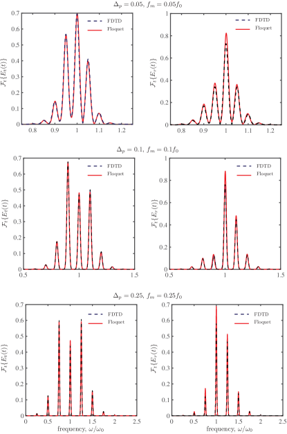
Figure 2: Spectrum of transmission and reflection fields from an infinite time-only ($\beta_{p}=0$) modulated metasurface incident with a normally incident plane-wave, for the case of a) $\Delta_{p}=0.05$, $\omega_{p}=0.05\omega_{0}$, b) $\Delta_{p}=0.1$, $\omega_{p}=0.1\omega_{0}$ and c) $\Delta_{p}=0.25$, $\omega_{p}=0.25\omega_{0}$. Total number of harmonics $2N+1=61$ and $T_{0}=100~{}$fs in (III-B). The metasurface parameters are: $\omega_{e0}=2\pi(224.63~{}\text{THz})$, $\omega_{ep}=0.36$ Trad/s, $\alpha_{e}=500\times 10^{9}$, $\omega_{m0}=2\pi(224.40~{}\text{THz})$, $\omega_{mp}=0.29$ Trad/s, $\alpha_{m}=100\times 10^{9}$, and excitation frequency $\omega_{0}=2\pi(230~{}\text{THz})$. The spectrum is normalized to the non-modulated case with $\Delta_{p}=0$.

While Fig. 2 showed results for few discrete points for $\Delta_{p}$ and $\Delta_{m}$, Fig. 3 shows a spectral map for a continuously varied modulation frequency $\omega_{p}$, for a given modulation depth $\Delta_{p}$. For simplicity, and considering the practical point of view, a perfectly matched metasurface with $\tilde{\chi}_{\text{ee}}=\tilde{\chi}_{\text{mm}}$ is assumed exhibiting zero reflections. The spectral map provides interesting and useful information about the interaction of the metasurface with the input fields. For example, at $\omega_{p}\approx 2\omega_{0}$, a substantial amplification of the fundamental frequency $\omega_{0}$ is observed, which is also the dominant spectral component in the transmitted fields. This is reminiscent of wave amplifications in diverse class of mechanical and electromagnetic parametric systems, where specific parameters of the system are modulated at twice the excitation frequency leading to wave instabilities [TamirST][OlinerST].

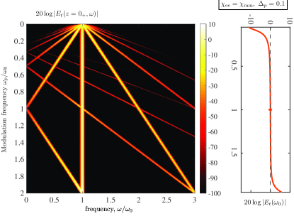
Figure 3: Transmission spectrum of a time-only modulated metasurface for a varying modulation frequency and fixed modulation depth, $\Delta_{p}$. The metasurface is assumed to be matched with $\chi_{\text{ee}}=\chi_{\text{mm}}$.

Next, an example of a space-time modulated metasurface is considered. Due to the spatial dependence of the susceptibilities following (6), the metasurface is spatially discretized and the Floquet analysis is performed at each $x$ location to determine the transmitted and reflected fields, $\tilde{E}_{t}(x,z=0_{+},\omega)$ and $\tilde{E}_{r}(x,z=0_{+},\omega)$, respectively. An example is shown in Fig. LABEL:Fig:Example, for an input Gaussian beam, showing the spectrum of the transmitted fields at the output of the metasurface at each location, with the mismatched parameters of Fig. 2. The Gaussian waveform nature is clearly observed for each spectral component. More interestingly, the phase profile across the metasurface as a function of frequency is also shown in Fig. LABEL:Fig:Example. A linear phase gradient with different spatial slopes, $d\angle E_{t}(x)/dx$, across the metasurface is clearly evident for each harmonic component, except the fundamental frequency. Therefore, each of these harmonics are expected to refract at different angles. Similar observations are also made for reflected fields (not shown here).