Changing U.S. Extreme Temperature Statistics

Abstract

The rise in global mean temperature is an incomplete description of warming. For many purposes, including agriculture and human life, temperature extremes may be more important than temperature means and changes in local extremes may be more important than mean global changes. We define a nonparametric statistic to describe extreme temperature behavior by quantifying the frequency of local daily all-time highs and lows, normalized by their frequency in the null hypothesis of no climate change. We average this metric over 1218 weather stations in the 48 contiguous United States, and find significantly fewer all-time lows than for the null hypothesis of unchanging climate. Record highs, by contrast, exhibit no significant trend. The metric is evaluated by Monte Carlo simulation for stationary and warming temperature distributions, permitting comparison of the statistics of historic temperature records with those of modeled behavior.

1 Introduction

The steady accumulation of greenhouse gases, most importantly CO₂, in the atmosphere and the warming trend it implies have been noted for more than a century and are the subject of a large literature (Hansen, 2006; Hansen et al., 2010; Intergovernmental Panel on Climate Change, 2013–2014). The extensive observational data are complemented by numerical climate simulations, in the form of General Circulation Models, whose unprecedented detail and resolution have been enabled by the revolution in high-performance computing.

On a day-to-day basis, we and our agriculture experience weather, not climate. The extremes of weather are important, independently of its mean (Katz & Brown, 1992; Karl et al., 1993; Nicholls, 1995; Easterling et al., 1997; Frich et al., 2002; Klein Tank & Können, 2003; Alexander et al., 2006; Platova, 2008; Meehl et al., 2009; Anderson & Kostinski, 2010; Rahmstorf & Coumou, 2011; Lewis et al., 2016). For example, the length of a growing season is often defined as the interval between the last vernal and first autumnal frosts. Heat stress on plants and animals, including people, is determined by peak temperatures rather than the mean temperature. Extreme temperatures can change independently of the mean temperature and its seasonal variation that we describe as climate.

All-time temperature highs and lows are particularly stressing. We define a nonparametric statistic that measures the frequency of all-time record highs or lows at a site on a specified calendar day. This statistic does not depend on a choice of a threshold, necessarily arbitrary, for a temperature excursion to be defined as extreme or stressing, but is an intrinsic and nondimensional property of the statistics of daily temperature variation.

In the null hypothesis of no climate change, the probability that the last daily maximum (or minimum) in a series of $N$ such maxima (or minima) sets an all-time record (assuming no ties) is $1/N$. By comparing the actual number of such all-time records in a database of 1218 sites in the 48 contiguous United States to the prediction of the null hypothesis, we describe changes in the frequency of the most thermally stressing events, information that is not contained in the trend of mean temperature. Averaging over these sites and over 365 calendar days permits extraction of statistically significant results from noisy data. The deviation of our metric from the value predicted by the null hypothesis is a measure of the change in frequency of extreme events. It also permits defining “equivalent warming rates” that describe trends in daily minima or maxima distinct from the mean rate of global warming. Comparison of these equivalent warming rates to the actual mean global warming rate compares (at the sites for which we have data) the rate of extreme events to that in the null hypothesis.

2 Methods

2.1 Data

The data in this study come from the United States Historical Climatology Network (CDIAC, 2015), a set of 1218 weather monitoring stations across the 48 contiguous United States, selected for quality by the National Climatic Data Center. The records include daily minimum and maximum temperatures, in whole degrees Fahrenheit, through the year 2014 and, for some sites, going back as far as 1850. We necessarily retain ^∘F ($1^{\,\circ}$C = $1.8^{\,\circ}$F) throughout the analysis because conversion to whole ^∘C would lose temperature resolution, while conversion to decimal ^∘C would produce nearly meaningless values in the tenths place.

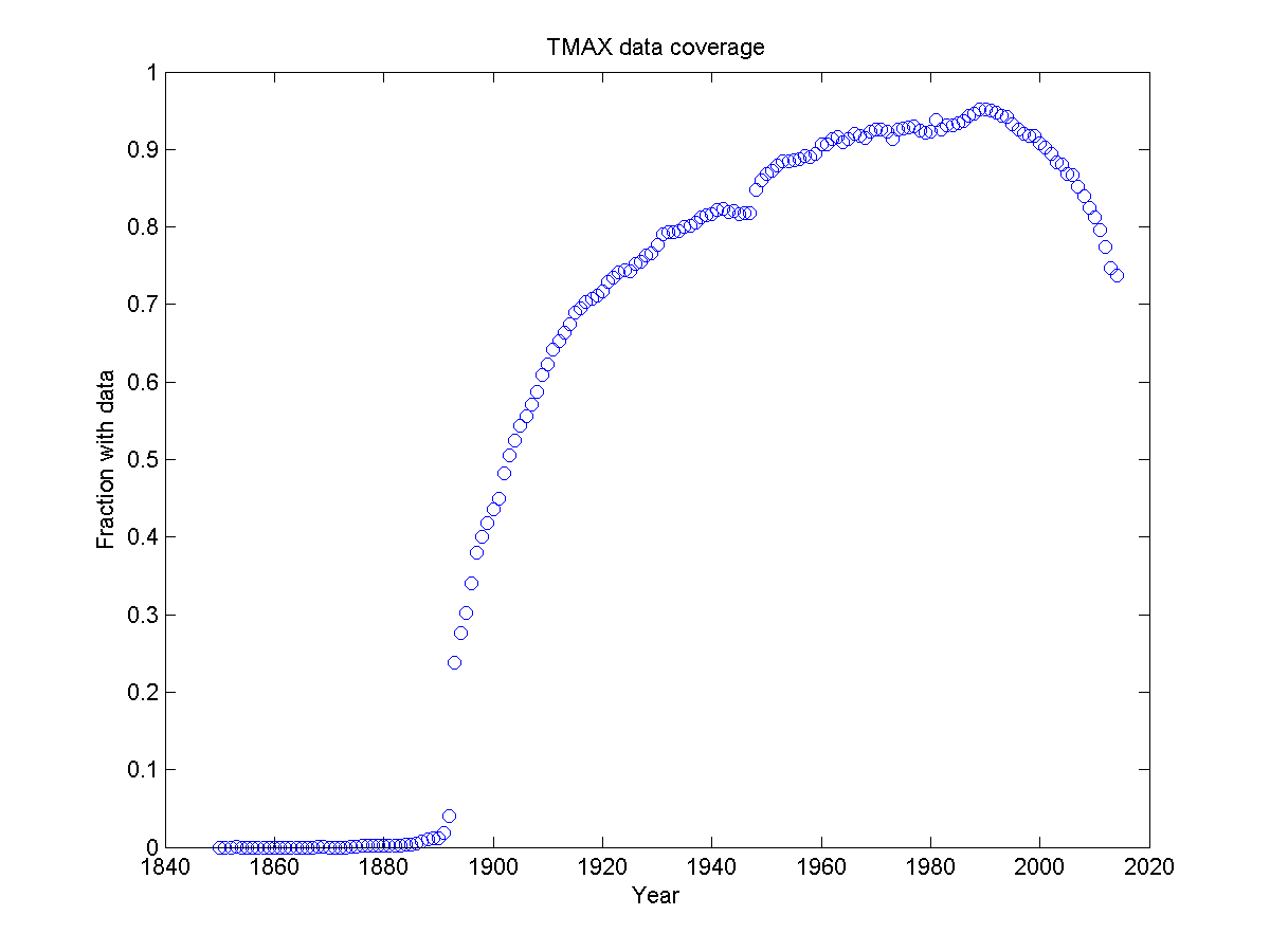
A year of full coverage would have one data point for each of 1218 stations on each of 365 days (February 29 data are ignored) for a total of 444,570 points. The actual data coverage is incomplete, especially for the early years. Approximately 40.96% of minima and 40.95% of maxima are missing. An additional 0.47% of minima and 0.43% of maxima were flagged as suspect y the NCDC for failing its consistency and homogeneity tests. As the flagged data make up a negligible portion of the dataset, we were able to use the NCDC’s strictest criteria in selecting data for quality, ignoring data with any flag whatsoever, without compromising data coverage. Because of these omissions, the overall data coverage from 1850 to 2014 is about 58%, with most of the missing data occurring in early years. Fig. 1 shows the fraction of these records actually extant each year. Annual coverage first exceeds 20% in 1893 and remains $>20\%$ thereafter. We therefore analyzed only data from 1893 onward; the overall data coverage for 1893–2014 is 79%.

Figure 1: Annual data coverage from 1850 to 2014, as a fraction of all $1218\times 365$ possible data points each year.

2.2 The Metric

Many metrics have been developed to describe the frequency and severity of extreme climate (Frich et al., 2002; Klein Tank & Können, 2003; Moberg et al., 2006). Most of these metrics involve necessarily arbitrary thresholds and definitions of extreme events, such as reference to particular percentiles in distributions of weather parameters or recurrence periods. We wish a metric that has no parameters or thresholds with arbitrary quantitative values and that produces a nonparametric statistical measure of the frequency of extreme events. This metric should permit ready comparison to the null hypothesis of a stationary climate, and its difference from its value in the null hypothesis should be interpretable as a nominal rate of warming. This nominal rate describes the change in frequency of extreme events, and is not the same as the mean warming rate; the difference in these rates is a measure of change in the severity of extreme events, distinct from the trend attributable to the mean warming itself.

The setting of a new maximum or minimum temperature record, for a given location and a given calendar day, may be defined as an extreme event. There are no arbitrary parameters in this definition, and the statistic that compare the frequency of such events to its value for the null hypothesis of a stationary climate is nonparametric. The metric is independent of the underlying temperature distribution and accommodates nonuniform data coverage.

We define two time series: $\eta(t)$ (the “high index”) and $\lambda(t)$ (the “low index”): Let $s\in\{1,2,\ldots,1218\}$ denote a weather monitoring station, $d\in\{1,2,\ldots,365\}$ denote a calendar day, and the whole number $t$ be the number of years since 1850 (the earliest year with a measurement at any station in our data set). $T(s,d,t)$ denotes the maximum temperature measured at site $s$, day $d$ and year $t$. The high index over these sites is defined as

$$\eta(t)=\frac{\sum_{s}\sum_{d}K(s,d,t)L(s,d,t)M(s,d,t)}{\sum_{s}\sum_{d}M(s,d,t)}$$ (1)

where

$$M(s,d,t)=\begin{cases}1&\text{There is a measured high temperature at }(s,d,t)\\ 0&\text{otherwise,}\end{cases}$$ (2)

$$L(s,d,t)=\sum_{t^{\prime}=0}^{t}M(s,d,t^{\prime}),$$ (3)

and

$$K(s,d,t)=\begin{cases}1&T(s,d,t)>T(s,d,t^{\prime})\ \text{for all }t^{\prime}<t\\ \frac{1}{n}&T(s,d,t)\text{ is an $n$-way tie for maximum among }t^{\prime}\leq t\\ 0&\text{otherwise.}\end{cases}$$ (4)

The “low index” $\lambda(t)$ is defined analogously, replacing $<$ with $>$ in the temperature test of Eq. 4 and letting $T$ denote the minimum temperature rather than the maximum. Even when there are gaps, our metric utilizes the information contained in all extant data because the likehood, in the null hypothesis of no climate change, that a new measurement will set a record is still $1/L(s,d,t)$, however many prior data may be missing.

These metrics measure the frequency of extreme (defined as record-setting) temperatures without making any assumptions about the distribution functions of daily maximum and minimum temperatures. In the null hypothesis of no warming, the maximum (or minimum) temperature measurement occurs at year $t$ with probability $1/L(s,d,t)$, which becomes the expected value of $K(s,d,t)$, so in Eq. 1 the numerator’s summand reduces, on average, to $M(s,d,t)$ and $\eta(t)$ and $\lambda(t)$ are, on average, unity, as desired. In an evolving climate the metrics’ differences from unity are useful nondimensional parametrizations of climate change. As the first measurement for any series is a new record by definition, $\lambda(1)\equiv\eta(1)\equiv 1$, independent of the temperature. In the following analysis of these time series, this initial unity value that carries no information is ignored to maximize sensitivity to climate trends.

$K$ is defined to account for ties for the record, which may occur because the data are discrete. If year $t$ is $n$-way tied for the record, there is a probability $1/n$ that the record (for the period 0–$t$) was indeed year $t$ rather than another of the tied years. In the null hypothesis of a stationary climate, any year (for which there are data) is equally likely to hold the record, so $K(s,d,t)$ has mean value $1/L(s,d,t)$. On average, then, $\eta(t)$ and $\lambda(t)$ would equal unity for all years $t$. Higher values indicate more frequent record-setting, while lower values indicate less frequent record-setting.

The indices can be computed for arbitrary subsets of the 1218 sites and arbitrary subsets of the calendar year, including single sites and single calendar days. Such calculations may reveal season- and region-specific trends that are otherwise obscured in the nationally averaged indicator.

2.3 Equivalent Warming Rates

If we know, or are willing to make some assumptions about, the distribution of daily minima and maxima about their (dependent on site and calendar day) means, we can describe the difference in the measured indices $\eta(t)$ and $\lambda(t)$ from unity (their values for a stationary climate) as an equivalent warming rate. To do this, we perform a Monte Carlo simulation of a uniformly warming climate for the period 1850–2014, using the observed mean warming rate of $0.010^{\,\circ}\text{F/y}=0.0055^{\,\circ}$C/y (Hansen, 2006; Hansen et al., 2010; Intergovernmental Panel on Climate Change, 2013–2014), assuming Gaussian distributions of daily minimum and maximum temperatures. The average (over sites and calendar days) standard deviations of the distributions of daily lows and highs are $8.15^{\,\circ}$F and $8.96^{\,\circ}$F respectively. The results are shown in Table 1 for several values of assumed standard deviations. To a good approximation, $1-\overline{\lambda}$ and $\overline{\eta}-1$ are inversely proportional to the assumed width of the distribution because they are the first terms in expansions in powers of the ratio of cumulative temperature change to the width.

Table 1: Indices of Lows and Highs in Simulated Warming of $0.010^{\,\circ}$F/y

Standard Deviation	$\overline{\lambda}$	$\overline{\eta}$
$5^{\,\circ}$F	$0.862\pm 0.008$	$1.153\pm 0.009$
$8.15^{\,\circ}$F	$0.913\pm 0.005$	$1.093\pm 0.005$
$8.96^{\,\circ}$F	$0.921\pm 0.005$	$1.085\pm 0.005$
$10^{\,\circ}$F	$0.930\pm 0.004$	$1.075\pm 0.004$
$15^{\,\circ}$F	$0.953\pm 0.003$	$1.048\pm 0.003$

We define “equivalent warming rates” for a measured mean index of highs $\overline{\eta}$

$$\left.{dT\over dt}\right|_{equiv,highs}\equiv{\overline{\eta}-1\over 1.085-1}\times 0.0055^{\,\circ}\text{C/y},$$ (5)

and of lows $\overline{\lambda}$

$$\left.{dT\over dt}\right|_{equiv,lows}\equiv{1-\overline{\lambda}\over 1-0.913}\times 0.0055^{\,\circ}\text{C/y}.$$ (6)

These equivalent warming rates are normalized so that they equal the actual mean warming rate if the indices equal those obtained in the Monte Carlo simulation. The ratios of equivalent warming rates to the actual mean warming rate (the fractions in Eqs. 5, 6) indicate whether extreme weather excursions, warm or cold, are becoming more or less frequent than they would be in the idealized model in which the distributions of temperature remain unchanged except for a constant rate of upward displacement.

3 Results

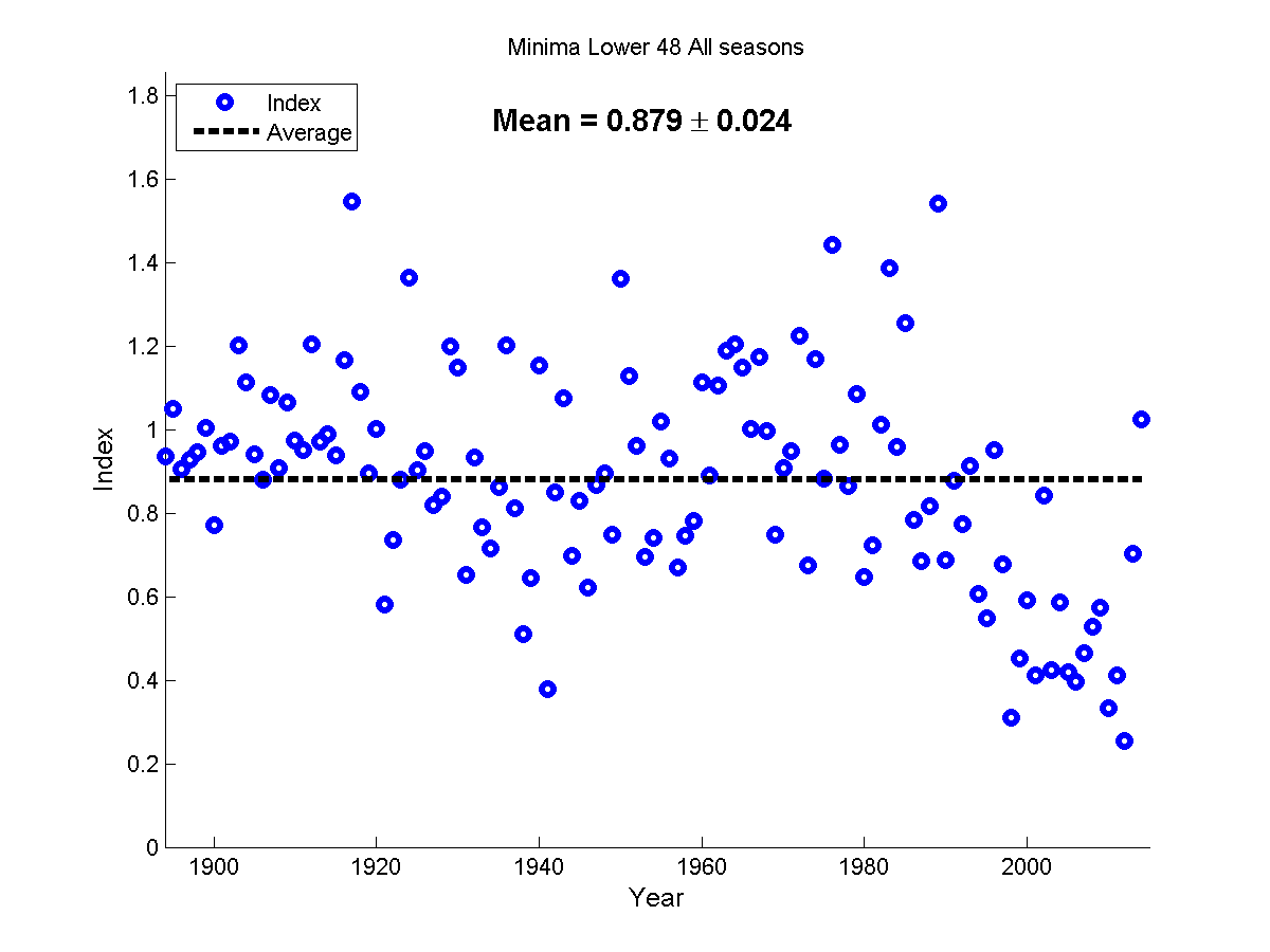
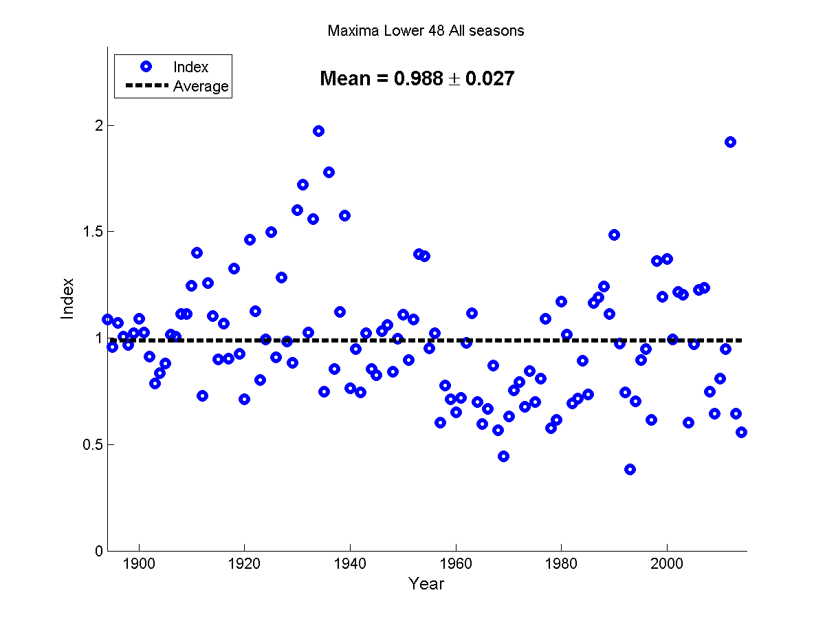
Fig. 2 shows $\lambda(t)$ and $\eta(t)$ computed over the 48 contiguous United States and the entire calendar year. The year-by-year values of $\lambda$ and $\eta$ are scattered, in part because geographical correlations among the 1218 sites and both day-to-day (weather system) and year-to-year temporal (ENSO, Decadal etc.) correlations reduce the effectiveness of averaging over the large dataset in smoothing random fluctuations; the $1218\times 365$ combinations of site and calendar day contain many fewer than $1218\times 365$ independent data. However, the means ($\overline{\lambda}$ and $\overline{\eta}$, averaged over the entire span of data excluding the first year, which is one by definition) have quite small uncertainties.

Figure 2: Indices of (a) minimum temperature records $\lambda(t)$ and (b) maximum temperature records $\eta(t)$ computed over all 1218 sites and all 365 calendar days, showing means and $\pm 1\sigma$.

A mean index greater (less) than unity occurs if temperature records are set more (less) often than expected in a stationary climate. We find that $\overline{\lambda}<1$ at the $5.0\sigma$ level. The mean maximum index $\overline{\eta}$ is consistent with unity (as in the null hypothesis of no climate change) All-time temperature minimum records are being set far less frequently than in a stationary climate, while maximum records are set at the same rate (to within statistical uncertainty) as in a stationary climate. This is consistent with the expectation that global warming tempers cold weather more than it intensifies hot weather (Karl et al., 1993; Intergovernmental Panel on Climate Change, 2013–2014).

These results can be interpreted in terms of the equivalent warming rates defined in Eqs. 5 and 6. Using the observed standard deviations of the daily lows and highs of $8.15^{\,\circ}$F and $8.96^{\,\circ}$F, respectively, the equivalent warming rates are

$$\left.{dT\over dt}\right|_{equiv,highs}=-0.0007\pm 0.0016^{\circ}\text{C/y}\quad\text{and}\quad\left.{dT\over dt}\right|_{equiv,lows}=0.0071\pm 0.0014\ ^{\circ}\text{C/y}.$$ (7)

The frequency of record lows is decreasing at about the same rate as would be expected from a simple displacement of all temperatures upward in time at the mean warming rate, but the frequency of record highs is not increasing at all, and is $3.9\sigma$ less than would be predicted by the hypothesis of uniform upward displacement of all temperatures.

The comparatively rapid warming of the last few decades is also evident in the $\lambda(t)$ data (Fig. 2a). If a period of rapid warming is followed by a period of stationary (but elevated, compared to the past) temperature, all-time record lows will continue to be unusually infrequent and all-time record highs unusually frequent during that period of stationary temperature until new records are set. The period 1990–2014 thus shows an intensification of the depressed $\lambda(t)$ found for the longer period 1893–2014. No systematic deviation of $\eta(t)$ from unity is found for either period.

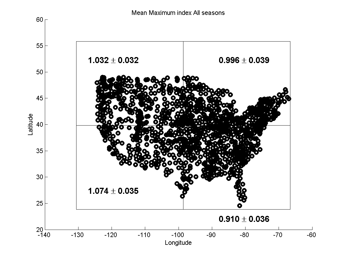
To obtain a more detailed regional picture, we split the 48 contiguous United States into four quadrants about their geographic center in Lebanon, Kansas at $39^{\circ}\ 50^{\prime}$N, $98^{\circ}\ 35^{\prime}$W, and show the locations of the sites and the results in Fig. 3. The subdivided values tell a more nuanced story than the nationally averaged values. In particular, the Southeast shows less warming than the other regions. It is the only quadrant where $\overline{\lambda}$ falls within $2\sigma$ of unity; it sets cold records at a rate that is consistent with a stationary climate, in contrast to the other regions. In the Southeast $\overline{\eta}$ is $2.5\sigma$ less than unity; hot records are set at a rate that is significantly less than that in a stationary climate. This result is consistent with the Southeastern “Warming Hole” identified by past analyses of climate data and simulations (Pan et al., 2004; Meehl et al., 2012). Even though the mean temperature in the Southeast is not decreasing, the rate of setting record temperature maxima there is suppressed compared to that suggested by its (nearly zero) mean temperature trend, a difference between equivalent and actual temperature trends like those found for the other three quadrants.

Figure 3: Mean index values and $1\sigma$ uncertainties in individual quadrants of the contiguous United States, for minima (a) and maxima (b). Each circle represents a single site. The sites are broadly distributed, with some, but not extreme, correlation with population density.

We also computed the indices for each season individually, both across the whole 48 contiguous United States and also subdivided into quadrants. The results are shown in Table 2 for $\overline{\lambda}$ and Table 3 for $\overline{\eta}$. In these tables “Winter” is defined as the first 92 days of the calendar year, and the subsequent seasons as subsequent 91 day periods. The Southeastern “Warming Hole” is evident in all seasons, with only a slight (and statistically not significantly different from zero) decrease in the rate of record minima but a $2.5\sigma$ ($3.3\sigma$ in Spring) decrease in the rate of maxima. In the other three quadrants the decreases in minima are generally very significant. In all quadrants, seasonal differences are not generally very significant; the trends (or absence of trends) are found year-round.

Table 2: Mean Minimum Index

Season	Southwest	Northwest	Southeast	Northeast	Lower 48
Winter	$0.820\pm 0.049$	$0.779\pm 0.052$	$0.925\pm 0.059$	$0.842\pm 0.056$	$0.851\pm 0.043$
Spring	$0.822\pm 0.035$	$0.838\pm 0.033$	$0.987\pm 0.043$	$0.855\pm 0.041$	$0.890\pm 0.030$
Summer	$0.804\pm 0.032$	$0.773\pm 0.030$	$0.970\pm 0.050$	$0.811\pm 0.037$	$0.853\pm 0.031$
Fall	$0.886\pm 0.040$	$0.925\pm 0.064$	$0.970\pm 0.063$	$0.880\pm 0.058$	$0.921\pm 0.045$
Whole Year	$0.833\pm 0.024$	$0.828\pm 0.029$	$0.963\pm 0.032$	$0.847\pm 0.030$	$0.879\pm 0.024$

Table 3: Mean Maximum Index

Season	Southwest	Northwest	Southeast	Northeast	Lower 48
Winter	$1.048\pm 0.063$	$1.093\pm 0.061$	$0.941\pm 0.054$	$1.173\pm 0.085$	$1.058\pm 0.047$
Spring	$1.142\pm 0.066$	$1.000\pm 0.058$	$0.833\pm 0.050$	$0.941\pm 0.056$	$0.951\pm 0.042$
Summer	$1.085\pm 0.046$	$1.068\pm 0.042$	$0.886\pm 0.074$	$0.839\pm 0.067$	$0.945\pm 0.046$
Fall	$1.023\pm 0.062$	$0.966\pm 0.056$	$0.980\pm 0.054$	$1.026\pm 0.063$	$0.997\pm 0.042$
Whole Year	$1.074\pm 0.035$	$1.032\pm 0.032$	$0.910\pm 0.036$	$0.996\pm 0.039$	$0.988\pm 0.027$

4 Discussion

We have defined a novel, robust and nonparametric measure of changes in the frequency of record high or low temperatures. This metric depends only on records of daily highs and lows. It differs from previously defined measures (Frich et al., 2002; Klein Tank & Können, 2003; Moberg et al., 2006; Shmakin & Popova, 2006; Platova, 2008) of temperature extremes by an absence of arbitrarily defined parameters and thresholds. Offsetting this advantage, it does not measure the magnitude of extremes, not differentiating a slight excursion beyond a previous all-time record from a large excursion.

Our work is most directly comparable to that of Meehl et al. (2009). They calculated the numbers of record daily highs and lows as functions of time for a world-wide, but very unevenly distributed (concentrated in the same region, the 48 contiguous United States, that we study), database covering the shorter period 1950–2006. They found fewer record lows than would be expected for a stationary climate, but about the same number of record highs, consistent with our results. They only considered the total numbers of temperature records, summed over sites and calendar days, in contrast to our treatment of data from each site and each day separately. This prevented them from extending their time base to earlier years for which only a fraction of sites have data or to sites with extensive missing data. Nor does their method permit quantitative averaging over the entire data period, although this can be approximated by “eyeball” from their figures. Such averaging smooths the scattered data, produces mean metrics with small statistical uncertainties, and permits quantitative evaluation of these uncertainties and of the significance of the results.

5 Conclusions

Applying our metrics to an extensive (1218 sites) database of daily temperature records from the 48 contiguous United States over the period 1893–2014, we find that the frequency of all-time lows decreased at a rate consistent with a uniform increase of temperatures at the rate of mean global warming. However, we find no significant change in the frequency of all-time highs, a result that differs from a modeled result for uniform warming at the rate of mean global warming by $4.9\sigma$. We also characterize changes in rates of temperature records in the well-known “Warming Hole” in the Southeastern United States, finding the same comparative suppression of record highs as found in the warming quadrants.

The result that global warming increases temperature minima more than maxima is expected (Hansen, 2006; Hansen et al., 2010; Intergovernmental Panel on Climate Change, 2013–2014), and is a natural consequence of the competing processes of energy transport. In cold weather energy is transported by radiation, and is subject to blanketing by greenhouse gases. In hot weather Solar radiation heats the Earth’s surface, producing instability and convective heat transfer that is little affected by atmospheric opacity. Although this qualitative effect is well-established, the fact that there would be no increase in temperature maxima, as measured by our metric $\eta$, was unexpected.

References

- Alexander et al. (2006) Alexander, L. V., Zhang, X., Peterson, T. C., et al. 2006, Global observed changes in daily climate extremes of temperature and precipitation, J. Geophys. Res., 111, D05109, doi:10.1029/2005JD006290
- Anderson & Kostinski (2010) Anderson, A., & Kostinski, A. 2010, Reversible record breaking and variability: temperature distributions across the globe, J. Appl. Meteor. Clim., 49, 1681
- CDIAC (2015) CDIAC. 2015, cdiac.ornl.gov/epubs/ndp/ushcn/background.html, accessed 10/10/2015; site will transition September, 2017
- Easterling et al. (1997) Easterling, D. R., Horton, B., Jones, P. D., et al. 1997, Maximum and minimum temperature trends for the globe, Science, 277, 364, doi:10.1126/science.277.5324.364
- Frich et al. (2002) Frich, P., Alexander, L. V., Della-Marta, P., et al. 2002, Observed coherent changes in climatic extremes during the second half of the twentieth century, Clim. Res., 19, 193
- Hansen et al. (2010) Hansen, J., Ruedy, R., Sato, M., & Lo, K. 2010, Global surface temperature change, Rev. Geophys., 48, RG4004, doi:10.1029/2010RG000345
- Hansen (2006) Hansen, J. et al. 2006, Global temperature change, Proc. Nat. Acad. Sci., 103, 14228
- Intergovernmental Panel on Climate Change (2013–2014) Intergovernmental Panel on Climate Change. 2013–2014, IPCC Fifth Assessment Report (IPCC), www.ipcc.ch/report/ar5/index.shtml
- Karl et al. (1993) Karl, T. R., Jones, P. D., Knight, R. W., et al. 1993, A new perspective of the recent global warming: asymmetric trends of daily maximum and minimum temperature, Bull. Am. Meteorol. Soc., 74, 1007
- Katz & Brown (1992) Katz, R. W., & Brown, B. G. 1992, Extreme events in a changing climate: variability is more important than averages, Clim. Chang., 21, 289, doi:10.1007/bf00139728
- Klein Tank & Können (2003) Klein Tank, A. M. G., & Können, G. P. 2003, Trends in indices of daily temperature and precipitation extremes in Europe, 1946–1999, J. Clim., 16, 3665
- Lewis et al. (2016) Lewis, S., King, A., & Perkins-Kirkpatrick, S. 2016, Defining a new normal for extremes in a warming world, Bull. Amer. Meteor. Soc., in press, doi:10.1175/BAMS-D-16-0183.1
- Meehl et al. (2012) Meehl, G. A., Arblaster, J. M., & Branstator, G. 2012, Mechanisms contributing to the warming hole and the consequent U. S. East-West differential of heat extremes, J. Clim., 25, 6394, doi:10.1175/JCLI-D-11-00655.1
- Meehl et al. (2009) Meehl, G. A., Tebaldi, C., Walton, G., Easterling, D., & McDaniel, L. 2009, Relative increase of record high maximum temperatures compared to record low minimum temperatures in the U.S., Geophys. Res. Lett., 36, L23701, doi:10.1029/2009GL040736
- Moberg et al. (2006) Moberg, A., Jones, P. D., Lister, D., et al. 2006, Indices for daily temperature and precipitation extremes in Europe analyzed for the period 1901–2000, J. Geophys. Res., 111, D22106, doi:10.1029/2006JD007103
- Nicholls (1995) Nicholls, N. 1995, Long-term climate monitoring and extreme events, Clim. Chang., 31, 231, doi:10.1007/bf01095148
- Pan et al. (2004) Pan, Z., Arritt, R. W., Takle, E. S., et al. 2004, Altered hydrologic feedback in a warming climate introduces a warming hole, Geophys. Res. Lett., 31, L17109, doi:10.1029/2004/GL020528
- Platova (2008) Platova, T. V. 2008, Annual air temperature extrema in the Russian federation and their climatic changes, Russ. Meteorol. Hydrol., 33, 735
- Rahmstorf & Coumou (2011) Rahmstorf, S., & Coumou, D. 2011, Increase of extreme events in a warming world, Pub. Natl. Acad. Sci., 108, 17905
- Shmakin & Popova (2006) Shmakin, A. B., & Popova, V. V. 2006, Dynamics of climate extremes in northern Eurasia in the late 20th century, Izvestija Atmos. Ocean. Phys., 42, 157