A Constructive Approach to High-dimensional Regression

Abstract

We develop a constructive approach to estimating sparse, high-dimensional linear regression models. The approach is a computational algorithm motivated from the KKT conditions for the $\ell_{0}$-penalized least squares solutions. It generates a sequence of solutions iteratively, based on support detection using primal and dual information and root finding. We refer to the algorithm as SDAR for brevity. Under a sparse Rieze condition on the design matrix and certain other conditions, we show that with high probability, the $\ell_{2}$ estimation error of the solution sequence decays exponentially to the minimax error bound in $O(\sqrt{J}\log(R))$ steps; and under a mutual coherence condition and certain other conditions, the $\ell_{\infty}$ estimation error decays to the optimal error bound in $O(\log(R))$ steps, where $J$ is the number of important predictors, $R$ is the relative magnitude of the nonzero target coefficients. Computational complexity analysis shows that the cost of SDAR is $O(np)$ per iteration. Moreover the oracle least squares estimator can be exactly recovered with high probability at the same cost if we know the sparsity level. We also consider an adaptive version of SDAR to make it more practical in applications. Numerical comparisons with Lasso, MCP and greedy methods demonstrate that SDAR is competitive with or outperforms them in accuracy and efficiency.

, , , and

1 Introduction

Consider the linear regression model

$$y=X\beta^{*}+\eta$$ (1.1)

where $y\in\mathbb{R}^{n}$ is a response vector, $X\in\mathbb{R}^{n\times p}$ is the design matrix with $\sqrt{n}$-normalized columns, $\beta^{*}=(\beta^{*}_{1},\ldots,\beta^{*}_{p})^{\prime}\in\mathbb{R}^{p}$ is the vector of underlying regression coefficients and $\eta\in\mathbb{R}^{n}$ is a vector of random errors with mean $0$ and variance $\sigma^{2}$. We focus on the case where $p\gg n$ and the model is sparse in the sense that only a relatively small number of predictors are important.

Without any constraints on $\beta^{*}$ there exist infinitely many least squares solutions for (1.1) since it is a highly undetermined linear system when $p\gg n$. These solutions usually over-fit the data. Under the assumption that $\beta^{*}$ is sparse in the sense that the number of important nonzero elements of $\beta^{*}$ is small relative to $n$, we can estimate $\beta^{*}$ by the solution of the $\ell_{0}$ minimization problem

$$\min_{\beta\in\mathbb{R}^{p}}\frac{1}{2n}\|X\beta-y\|^{2}_{2},\quad\textrm{subject to}\quad\|\beta\|_{0}\leq s,$$ (1.2)

where $s>0$ controls the sparsity level. However, (1.2) is generally NP hard [Natarajan (1995)], hence it is challenging to design a stable and fast algorithm to solve it.

In this paper we propose a constructive approach to estimating (1.1). The approach is a computational algorithm motivated from the necessary KKT conditions for the Lagrangian form of (1.2). It finds an approximate sequence of solutions to the KKT equations iteratively using a support detection and root finding method until convergence is achieved. For brevity, we refer to the proposed approach as SDAR.

1.1 Literature review

Several approaches have been proposed to approximate (1.2). Among them the Lasso [Tibshirani (1996), Chen, Donoho and Saunders (1998)], which uses the $\ell_{1}$ norm of $\beta$ in the constraint instead of the $\ell_{0}$ norm in (1.2), is a popular method. Under the irrepresentable condition on the design matrix $X$ and a sparsity assumption on $\beta^{*}$, Lasso is model selection (and sign) consistent [Meinshausen and Bühlmann (2006), Zhao and Yu (2006), Wainwright (2009)]. Lasso is a convex minimization problem. Several fast algorithms have been proposed, including LARS (Homotopy) [Osborne, Presnell and Turlachet (2000), Efron et al. (2004), Donoho and Tsaig (2008)], coordinate descent [Fu (1998), Friedman et al. (2007), Wu and Lange (2008)], and proximal gradient descent [Agarwal, Negahban and Wainwright (2012), Xiao and Zhang (2013), Nesterov (2013)].

However, Lasso tends to overshrink large coefficients, which leads to biased estimates [Fan and Li (2001), Fan and Peng (2004)]. The adaptive Lasso proposed by Zou (2006) and analyzed by Huang, Ma and Zhang (2008) in high-dimensions can achieve the oracle property under certain conditions. But its requirements on the minimum value of the nonzero coefficients are not optimal. Nonconvex penalties such as the smoothly clipped absolute deviation (SCAD) penalty [Fan and Li (2001)], the minimax concave penalty (MCP) [Zhang (2010a)], and the capped $\ell_{1}$ penalty [Zhang (2010b)] were adopted to remedy these problems. Although the global minimizers (also there exist some local minimizers) of these nonconvex regularized models can eliminate the estimation bias and enjoy the oracle properties [Zhang and Zhang (2012)], computing their global minimizers or local minimizers with the desired statistical properties is challenging since the optimization problem is nonconvex, nonsmooth and large scale in general.

There are several numerical algorithms for nonconvex regularized problems. The first kind of such methods can be considered a special case (or variant) of minimization-maximization algorithm [Lange, Hunter and Yang (2000), Hunter and Li (2005)] or of multi-stage convex relaxation [Zhang (2010b)]. Examples include local quadratic approximation (LQA) [Fan and Li (2001)], local linear approximation (LLA) [Zou and Li (2008)], decomposing the penalty into a difference of two convex terms (CCCP) [Kim, Cho and Oh (2008), Gasso, Rakotomamonjy and Canu (2009)]. The second type of methods is the coordinate descent algorithms, including coordinate descent of the Gauss-Seidel version [Breheny and Huang (2011), Mazumder et al. (2011)] and coordinate descent of the Jacobian version, i.e., the iterative thresholding method [Blumensath and Davies (2008), She (2009)]. These algorithms generate a sequence at which the objective functions are nonincreasing, but the convergence of the sequence itself is generally unknown. Moreover, if the sequence generated from multi-stage convex relaxation (starts from a Lasso solution) converges, it converges to some stationary point which may enjoy certain oracle statistical properties [Zhang (2010b), Fan, Xue and Zou (2014)] with the cost of a Lasso solver per iteration. Jiao, Jin and Lu (2013) proposed a globally convergent primal dual active set algorithm for a class of nonconvex regularized problems. Recently, there has been much effort to show that CCCP, LLA and the path following proximal-gradient method can track the local minimizers with the desired statistical properties [Wang, Kim and Li (2013), Fan, Xue and Zou (2014), Wang, Liu and Zhang (2014) and Loh and Wainwright (2015)].

Another line of research includes greedy methods such as the orthogonal match pursuit (OMP) [Mallat and Zhang (1993)] for solving (1.2) approximately. The main idea is to iteratively select one variable with the strongest correlation with the current residual at a time. Roughly speaking, the performance of OMP can be guaranteed if the small submatrices of $X$ are well conditioned like orthogonal matrices [Tropp (2004), Donoho, Elad and Temlyakov (2006), Cai and Wang (2011), Zhang (2011a)]. Fan and Lv (2008) proposed a marginal correlation learning method called sure independence screening (SIS), see also Huang, Horowitz and Ma (2008) with an equivalent formulation that uses penalized univariate regression for screening. Fan and Lv (2008) recommended an iterative SIS to improve the finite-sample performance. As they discussed the iterative SIS also uses the core idea of OMP but it can select more features at each iteration. There are several more recently developed greedy methods aimed at selecting several variables a time or removing variables adaptively, such as hard thresholding gradient descent (GraDes) [Garg and Khandekar (2009)], stagewise OMP (StOMP) [Donoho et al. (2012)], adaptive forward-backward selection (FoBa) [Zhang (2011b)].

1.2 Contributions

SDAR is a new approach for fitting sparse, high-dimensional regression models. Compared with the penalized methods, SDAR does not aim to minimize any regularized criterion, instead, it constructively generates a sequence of solutions $\{\beta^{k},k\geq 1\}$ to the KKT equations of the $\ell_{0}$ penalized criterion. SDAR can be viewed as a primal-dual active set method for solving the $\ell_{0}$ regularized least squares problem with a changing regularization parameter $\lambda$ in each iteration (this will be explained in detail in Section 2). However, the sequence generated by SDAR is not a minimizing sequence of the $\ell_{0}$ regularized least squares criterion. Compared with the greedy methods, the features selected by SDAR are based on the sum of the primal (current approximation $\mathbf{\beta}^{k}$) and the dual information (current correlation $d^{k}=X^{\prime}(y-X\mathbf{\beta}^{k})/n$), while greedy methods only use dual information. The differences between SDAR and several greedy methods will be explained in more detail in Subsection 6.

We show that SDAR achieves sharp estimation error bounds in finite iterations. Specifically, we show that: (a) under a sparse Rieze condition on $X$ and a sparsity assumption on $\beta^{*}$, $\|\beta^{k}-\mathbf{\beta}^{*}\|_{2}$ achieves the minimax error bound up to a constant factor with high probability in $O(\sqrt{J}\log(R))$ steps; (b) under a mutual coherence condition on $X$ and a sparsity assumption on $\beta^{*}$, the $\|\beta^{k}-\mathbf{\beta}^{*}\|_{\infty}$ achieves the optimal error bound $O(\sigma\sqrt{\log(p)/n})$ in $O(\log(R))$ steps, where $J$ is the number of important predictors, $R$ is the relative magnitude of the nonzero target coefficients (the exact definitions of $J$ and $R$ are given in Section 3); (c) under the conditions in (a) and (b), with high probability, $\beta^{k}$ coincides with the oracle least squares estimator in $O(\sqrt{J}\log(R))$ and $O(\log(R))$ iterations, respectively, if $J$ is available and the minimum magnitude of the nonzero elements of $\beta^{*}$ is of the order $O(\sigma\sqrt{2\log(p)/n})$, which is the optimal magnitude of detectable signal.

An interesting aspect of the result in (b) is that the number of iterations for SDAR to achieve the optimal error bound is $O(\log(R))$, which does not depend on the underlying sparsity level. This is an appealing feature for the problems with a large triple $(n,p,J)$. We also analyze the computational cost of SDAR and show that it is $O(np)$ per iteration, comparable to the existing penalized and greedy methods.

In summary, the main contributions of this paper are as follows.

• We proposed a new approach to fitting sparse, high-dimensional regression models. Unlike the existing penalized methods that approximate the $\ell_{0}$ penalty using the $\ell_{1}$ or its concave modifications, the proposed approach seeks to directly approximate the solutions to the $\ell_{0}$ penalized problem.

• We show that the sequence of solutions $\{\beta^{k},k\geq 1\}$ generated by the SDAR achieves sharp error bounds. An interesting aspect of our results is that these bounds can be achieved in $O(\sqrt{J}\log(R))$ or $O(\log(R))$ iterations.

• We also consider an adaptive version of SDAR, named ASDAR, by tuning the size of the fitted model based on a data driven procedure such as the BIC. Our simulation studies demonstrate that SDAR/ ASDAR outperforms the Lasso, MCP and several greedy methods in terms of accuracy and efficiency.

1.3 Notation

Let $\|\beta\|_{q}=(\sum_{i=1}^{p}|\beta_{i}|^{q})^{1/q},q\in[1,\infty],$ be the $q$-norm of a column vector $\beta=(\beta_{1},\ldots,\beta_{p})^{\prime}\in\mathbb{R}^{p}$. We denote the number of nonzero elements of $\beta$ by $\|\beta\|_{0}$. We denote the operator norm of $X$ induced by the vector 2-norm by $\left\|X\right\|$. We use E to denote the identity matrix. 0 denotes a column vector in $\mathbb{R}^{p}$ or a matrix with elements all 0. Let $S=\{1,2,...,p\}$. For any $A,B\subseteq S$ with length $|A|,|B|$, we denote $\beta_{A}=(\beta_{i},i\in A)\in\mathbb{R}^{|A|}$, $X_{A}=(X_{i},i\in A)\in\mathbb{R}^{n\times|A|}$. And $X_{AB}\in\mathbb{R}^{|A|\times|B|}$ denotes a submatrix of $X$ whose rows and columns are listed in $A$ and $B$, respectively. We define $\beta|_{A}\in\mathbb{R}^{p}$ with its $i$-th element $(\beta|_{A})_{i}=\beta_{i}\textbf{1}(i\in A)$, where $\textbf{1}(\cdot)$ is the indicator function. We denote the support of $\beta$ by $\textrm{supp}(\beta)$. Define $A^{*}=\textrm{supp}(\mathbf{\beta}^{*})$ and $K={\|\mathbf{\beta}^{*}\|}_{0}$. We use $\|\beta\|_{k,\infty}$ and $\left|\beta\right|_{\textrm{min}}$ to denote the $k$-th largest elements (in absolute value) of $\beta$ and the minimum absolute value of $\beta$, respectively.

1.4 Organization

In Section 2 we develop the SDAR algorithm based on the necessary conditions for the $\ell_{0}$ penalized solutions. In Section 3 we establish the nonasymptotic error bounds of the SDAR solutions. In Section 4 we describe a data driven adaptive SDAR. In Section 5 we analyze the computational complexity of SDAR and ASDAR and discuss the relationship of SDAR with several greedy methods and screening method. In Section 6 we conduct simulation studies to demonstrate the performance of SDAR/ ASDAR by comparing it with Lasso, MCP and several greedy methods. We conclude in Section 7 with some final remarks. The proofs are given in the Appendix.

2 Derivation of SDAR

In this section we describe the SDAR algorithm. Consider the Lagrangian form of the $\ell_{0}$ regularized minimization problem (1.2),

$$\min_{\mathbf{\beta}\in\mathbb{R}^{p}}\frac{1}{2n}{\|X\mathbf{\beta}-y\|}_{2}^{2}+\lambda{\|\mathbf{\beta}\|}_{0}.$$ (2.1)

Lemma 2.1.

Let $\beta^{\diamond}$ be a minimizer of (2.1). Then $\beta^{\diamond}$ satisfies:

$$\begin{cases}d^{\diamond}=X^{\prime}(y-X\beta^{\diamond})/n,\\ \beta^{\diamond}=H_{\lambda}(\beta^{\diamond}+d^{\diamond}),\end{cases}$$ (2.2)

where $H_{\lambda}(\cdot)$ is the hard thresholding operator defined by

$$(H_{\lambda}(\beta))_{i}=\begin{cases}\textrm{0},&\text{if $|\beta_{i}|<\sqrt{2\lambda}$},\\ \text{$\beta_{i}$},&\text{if $|\beta_{i}|\geq\sqrt{2\lambda}$}.\end{cases}$$ (2.3)

Conversely, if $\beta^{\diamond}$ and $d^{\diamond}$ satisfy (2.2), then $\beta^{\diamond}$ is a local minimizer of (2.1).

Remark 2.1.

Lemma 2.1 gives the KKT condition of the $\ell_{0}$ regularized minimization problem (1.2), similar results for SCAD MCP capped-$\ell_{1}$ regularized least squares models can be derived by replacing the hard thresholding operator in (2.2) with their corresponding thresholding operators, see Jiao, Jin and Lu (2013) for details.

Let $A^{\diamond}=\textrm{supp}(\beta^{\diamond})$ and $I^{\diamond}=(A^{\diamond})^{c}$. Suppose that the rank of $X_{A^{\diamond}}$ is $|A^{\diamond}|$. From the definition of $H_{\lambda}(\cdot)$ and (2.2) it follows that

$$A^{\diamond}=\Big{\{}i\in S\big{|}\left|\beta^{\diamond}_{i}+d^{\diamond}_{i}\right|\geq\sqrt{2\lambda}\Big{\}},\quad I^{\diamond}=\Big{\{}i\in S\big{|}\left|\beta^{\diamond}_{i}+d^{\diamond}_{i}\right|<\sqrt{2\lambda}\Big{\}},$$

and

$$\left\{\begin{aligned} \beta^{\diamond}_{I^{\diamond}}&=\textbf{0},\\ d^{\diamond}_{A^{\diamond}}&=\textbf{0},\\ \beta^{\diamond}_{A^{\diamond}}&=(X_{A^{\diamond}}^{\prime}X_{A^{\diamond}})^{-1}X_{A^{\diamond}}^{\prime}y,\\ d^{\diamond}_{I^{\diamond}}&=X^{\prime}_{I^{\diamond}}(y-X_{A^{\diamond}}\beta^{\diamond}_{A^{\diamond}})/n.\end{aligned}\right.$$

We solve this system of equations iteratively. Let $\{\mathbf{\beta}^{k},d^{k}\}$ be the solution at the $k$th iteration. We approximate $\{A^{\diamond},I^{\diamond}\}$ by

$$A^{k}=\Big{\{}i\in S\big{|}|\mathbf{\beta}^{k}_{i}+d^{k}_{i}|\geq\sqrt{2\lambda}\Big{\}},\quad I^{k}=(A^{k})^{c}.$$ (2.4)

Then we can obtain a new approximation pair $(\mathbf{\beta}^{k+1},d^{k+1})$ by

$$\left\{\begin{aligned} \mathbf{\beta}^{k+1}_{I^{k}}&=\textbf{0},\\ d^{k+1}_{A^{k}}&=\textbf{0},\\ \mathbf{\beta}^{k+1}_{A^{k}}&=(X_{A^{k}}^{\prime}X_{A^{k}})^{-1}X_{A^{k}}^{\prime}y,\\ d^{k+1}_{I^{k}}&=X^{\prime}_{I^{k}}(y-X_{A^{k}}\mathbf{\beta}^{k+1}_{A^{k}})/n.\end{aligned}\right.$$ (2.5)

Now suppose we want the support of the solutions to have size $T\geq 1$. We can choose

$$\sqrt{2\lambda}\triangleq\|{\mathbf{\beta}^{k}+d^{k}}\|_{T,\infty}$$ (2.6)

in (2.4). With this choice of $\lambda$, we have $|A^{k}|=T,k\geq 1.$ Then with an initial $\beta^{0}$ and using (2.4) and (2.5) with the $\lambda$ in (2.6), we obtain a sequence of solutions $\{\beta^{k},k\geq 1\}$.

There are two key aspects of SDAR. In (2.4) we detect the support of the solution based on the sum of the primal ($\mathbf{\beta}^{k}$) and dual ($d^{k}$) approximations and, in (2.5) we calculate the nonzero solution on the detected support. Therefore, SDAR can be considered an iterative method for solving the KKT equations (2.2) with an important modification: a different $\lambda$ value given in (2.6) in each step of the iteration is used. Thus we can also view SDAR as an adaptive thresholding and least-squares fitting procedure that uses both the primal and dual information. We summarize SDAR in Algorithm 1.

Remark 2.2.

If $A^{k+1}=A^{k}$ for some $k$ we stop SDAR since the sequences generated by SDAR will not change. Under certain conditions, we will show that $A^{k+1}=A^{k}=\textrm{supp}(\beta^{*})$ if $k$ is large enough, i.e., the stop condition in SDAR will be active and the output is the oracle estimator when it stops.

As an example, Figure 1 shows the solution path of SDAR with $T=1,2,\ldots,5K$, the MCP and the Lasso paths on $5K$ different $\lambda$ values for a data set generated from a model with $(n=50,p=100,K=5,\sigma=0.3,\rho=0.5,R=10)$, which will be described in Section 6. The Lasso path is computed using LARS [Efron et al. (2004)]. Note that the SDAR path is a function of the fitted model size $T=1,\ldots,L$, where $L$ is the size of the largest fitted model. In comparison, the paths of MCP and Lasso are functions of the penalty parameter $\lambda$ in prespecified interval. In this example, SDAR selects the first $T$ largest components of $\mathbf{\beta}^{*}$ correctly when $T\leq K$.

Algorithm 1 Support detection and root finding (SDAR)

0:  $\beta^{0}$, $d^{0}=X^{\prime}(y-X\beta^{0})/n$, $T$; set $k=0$.

1:  for $k=0,1,2,\cdots$ do

2:     $A^{k}=\{i\in S\big{|}|\beta^{k}_{i}+d^{k}_{i}|\geq\|\beta^{k}+d^{k}\|_{T,\infty}\},\quad I^{k}=(A^{k})^{c}$

3:     $\mathbf{\beta}^{k+1}_{I^{k}}=\textbf{0}.$

4:     $d^{k+1}_{A^{k}}=\textbf{0}.$

5:     $\mathbf{\beta}^{k+1}_{A^{k}}=(X_{A^{k}}^{\prime}X_{A^{k}})^{-1}X_{A^{k}}^{\prime}y.$

6:     $d^{k+1}_{I^{k}}=X^{\prime}_{I^{k}}(y-X_{A^{k}}\mathbf{\beta}^{k+1}_{A^{k}})/n.$

7:     if $A^{k+1}=A^{k}$, then

8:        Stop and denote the last iteration by $\beta_{\hat{A}},\beta_{\hat{I}},d_{\hat{A}},d_{\hat{I}}$;

9:     else

10:        $k=k+1$.

11:     end if

12:  end for

12:  $\hat{\beta}=(\beta_{\hat{A}}^{\prime},\beta_{\hat{I}}^{\prime})^{\prime}$as the estimates of $\beta^{*}$.

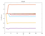
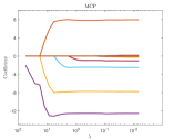
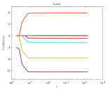
Figure 1: The solution paths of SDAR, MCP and Lasso.

3 Nonasymptotic error bounds

In this section we present the nonasymptotic $\ell_{2}$ and $\ell_{\infty}$ error bounds for the solution sequence generated by SDAR as given in Algorithm 1.

We say that $X$ satisfies the SRC [Zhang and Huang (2008), Zhang (2010a)] with order $s$ and spectrum bounds $\{c_{-}(s),c_{+}(s)\}$ if

$$0<c_{-}(s)\leq\frac{{\|X_{A}u\|}_{2}^{2}}{n{\|u\|}_{2}^{2}}\leq c_{+}(s)<\infty,\forall\,{0}\neq u\in\mathbb{R}^{\left|A\right|}\mbox{ with }A\subset S\mbox{ and }\left|A\right|\leq s.$$

We denote this condition by $X\sim\textrm{SRC}\{s,c_{-}(s),c_{+}(s)\}$. The SRC gives the range of the spectrum of the diagonal sub-matrices of the Gram matrix $G=X^{\prime}X/n$. The spectrum of the off diagonal sub-matrices of $G$ can be bounded by the sparse orthogonality constant $\theta_{a,b}$ defined as the smallest number such that

$$\theta_{a,b}\geq\frac{{\|X_{A}^{\prime}X_{B}u\|}_{2}}{n{\|u\|}_{2}},\forall\,\textrm{0}\neq u\in\mathbb{R}^{\left|B\right|}\mbox{ with }A,B\subset S,\left|A\right|\leq a,\left|B\right|\leq b,\mbox{ and }A\cap B=\emptyset.$$

Another useful quantity is the mutual coherence $\mu$ defined as $\mu=\max_{i\neq j}\left|G_{i,j}\right|$, which characterizes the minimum angle between different columns of $X/\sqrt{n}$. Some useful properties of these quantities are summarized in Lemma 9.1 in the Appendix.

In addition to the regularity conditions on the design matrix, another key condition is the sparsity of the regression parameter $\mathbf{\beta}^{*}$. The usual sparsity condition is to assume that the regression parameter $\mathbf{\beta}^{*}_{i}$ is either nonzero or zero and that the number of nonzero coefficients is relatively small. This strict sparsity condition is not realistic in many problems. Here we allow that $\mathbf{\beta}^{*}$ may not be strictly sparse but most of its elements are small. Let $A^{*}_{J}=\{i\in S:|\mathbf{\beta}^{*}_{i}|\geq\|\mathbf{\beta}^{*}\|_{J,\infty}\}$ be the set of the indices of the first $J$ largest components of $\mathbf{\beta}^{*}$. Typically, we have $J\ll n$. Let

$$R=\frac{\bar{M}}{\bar{m}},$$ (3.1)

where $\bar{m}=\min\{|\mathbf{\beta}^{*}_{i}|,i\in A^{*}_{J}\}$ and $\bar{M}=\max\{|\mathbf{\beta}^{*}_{i}|,i\in A^{*}_{J}\}$. Since $\mathbf{\beta}^{*}=\mathbf{\beta}^{*}|_{A^{*}_{J}}+\mathbf{\beta}^{*}|_{(A^{*}_{J})^{c}}$, we can transform the non-exactly sparse model (1.1) to the following exactly sparse model by including the small components of $\beta^{*}$ in the noise,

$$y=X\bar{\beta}^{*}+\bar{\eta},$$ (3.2)

where

$$\bar{\beta}^{*}=\mathbf{\beta}^{*}|_{A^{*}_{J}}\ \mbox{ and }\ \bar{\eta}=X\mathbf{\beta}^{*}|_{(A^{*}_{J})^{c}}+\eta.$$ (3.3)

Let $R_{J}={\|\mathbf{\beta}^{*}|_{(A^{*}_{J})^{c}}\|}_{2}+{\|\mathbf{\beta}^{*}|_{(A^{*}_{J})^{c}}\|}_{1}/\sqrt{J}$, which is a measure of the magnitude of the small components of $\mathbf{\beta}^{*}$ outside $A^{*}_{J}$. Of course, $R_{J}=0$ if $\mathbf{\beta}^{*}$ is exactly $K$-sparse with $K\leq J$. Without loss of generality, we let $J=K$, $m=\bar{m}$ and $M=\bar{M}$ for simplicity if $\mathbf{\beta}^{*}$ is exactly $K$-sparse.

Let $\beta^{J,o}$ be the oracle estimator defined as $\beta^{J,o}=\arg\min_{\beta}\{\frac{1}{2n}\|y-X\beta\|_{2}^{2},\beta_{j}=0,j\not\in A^{*}_{J}\}$, that is, $\beta^{J,o}_{A^{*}_{J}}=X_{A^{*}_{J}}^{{\dagger}}y$ and $\beta^{J,o}_{(A^{*}_{J})^{c}}=\textbf{0}$, where $X_{A^{*}_{J}}^{{\dagger}}$ is the generalized inverse of $X_{A^{*}_{J}}$ and equals to $(X_{A^{*}_{J}}^{\prime}X_{A^{*}_{J}})^{-1}X_{A^{*}_{J}}^{\prime}$ if $X_{A^{*}_{J}}$ is of full column rank. So $\beta^{J,o}$ is obtained by keeping the predictors corresponding to the $J$ largest components of $\mathbf{\beta}^{*}$ in the model and dropping the other predictors. Obviously, $\beta^{J,o}=\beta^{o}$ if $\mathbf{\beta}^{*}$ is exactly $K$-sparse, where $\beta^{o}_{A^{*}}=X_{A^{*}}^{{\dagger}}y,\beta^{o}_{(A^{*})^{c}}=\textbf{0}$.

3.1 $\ell_{2}$ error bounds

Let $1\leq T\leq p$ be a given integer used in Algorithm 1. We require the following basic assumptions on the design matrix $X$ and the error vector $\eta$.

(A1) The input integer $T$ used in Algorithm 1 satisfies $T\geq J$.

(A2) $X\sim\text{SRC}\{2T,c_{-}(2T),c_{+}(2T)\}$.

(A3) The random errors $\eta_{1},\ldots,\eta_{n}$ are independent and identically distributed with mean zero and sub-Gaussian tails, that is, there exists a $\sigma\geq 0$ such that $E[\exp(t\eta_{i})]\leq\exp(\sigma^{2}t^{2}/2)$ for $t\in\mathbb{R}^{1}$, $i=1,\ldots,n.$

Let

$$\gamma=\frac{2\theta_{T,T}+(1+\sqrt{2})\theta_{T,T}^{2}}{c_{-}(T)^{2}}+\frac{(1+\sqrt{2})\theta_{T,T}}{c_{-}(T)}.$$

Define $h_{2}(T)=\max_{A\subseteq S:|A|\leq T}{\|X_{A}^{\prime}\bar{\eta}\|}_{2}/n$, where $\bar{\eta}$ is defined in (3.3).

Theorem 3.1.

Let $1\leq T\leq p$ be a given integer used in Algorithm 1. Suppose $\gamma<1$.

• Assume (A1) and (A2) hold. We have

  $${\|\bar{\beta}^{*}|_{A_{J}^{*}\backslash A^{k+1}}\|}_{2} \leq\gamma^{k+1}{\|\bar{\beta}^{*}\|}_{2}+\frac{\gamma}{(1-\gamma)\theta_{T,T}}h_{2}(T),$$ (3.4)

  $${\|\mathbf{\beta}^{k+1}-\bar{\beta}^{*}\|}_{2} \leq b_{1}\gamma^{k}{\|\bar{\beta}^{*}\|}_{2}+b_{2}h_{2}(T),$$ (3.5)

  where

  $$b_{1}=1+\frac{\theta_{T,T}}{c_{-}(T)}\ \mbox{ and }\ b_{2}=\frac{\gamma}{(1-\gamma)\theta_{T,T}}b_{1}+\frac{1}{c_{-}(T)}.$$ (3.6)

• Assume (A1)-(A3) hold. Then for any $\alpha\in(0,1/2)$, with probability at least $1-2\alpha$,

  $${\|\bar{\beta}^{*}|_{A_{J}^{*}\backslash A^{k+1}}\|}_{2} \leq\gamma^{k+1}{\|\bar{\beta}^{*}\|}_{2}+\frac{\gamma}{(1-\gamma)\theta_{T,T}}\varepsilon_{1},$$ (3.7)

  $${\|\mathbf{\beta}^{k+1}-\bar{\beta}^{*}\|}_{2} \leq b_{1}\gamma^{k}{\|\bar{\beta}^{*}\|}_{2}+b_{2}\varepsilon_{1},$$ (3.8)

  where $\varepsilon_{1}=c_{+}(J)R_{J}+\sigma\sqrt{T}\sqrt{2\log(p/\alpha)/n}.$

Remark 3.1.

Assumption (A1) is necessary for SDAR to select at least $J$ nonzero features. The sparse Riesz condition in (A2) has been used in the analysis of the Lasso and MCP [Zhang and Huang (2008), Zhang (2010a)]. Let $c(T)=(1-c_{-}(2T))\vee(c_{+}(2T)-1)$, which is closely related to the the RIP (restricted isometry property) constant $\delta_{2T}$ for $X$ [Candès and Tao (2005)]. By (9.5) in the Appendix, it can be verified that a sufficient condition for $\gamma<1$ is $c(T)\leq 0.1599$, i.e., $c_{+}(2T)\leq 1.1599$, $c_{-}(2T)\geq 0.8401$. The sub-Gaussian condition (A3) is often assumed in the literature and slightly weaker than the standard normality assumption.

Remark 3.2.

Several greedy algorithms have also been studied under the assumptions related to the sparse Riesz condition. For example, Zhang (2011b) studied OMP under the condition $c_{+}(T)/c_{-}(31T)\leq 2$. Zhang (2011a) analyzed the forward-backward greedy algorithm (FoBa) under the condition $8(T+1)\leq(s-2)Tc_{-}^{2}(sT)$, where $s>0$ is a properly chosen parameter. GraDes [Garg and Khandekar (2009)] has been analyzed under the RIP condition $\delta_{2T}\leq 1/3$. These conditions and (A2) are related but do not imply each other. The order of $\ell_{2}$-norm estimation error of SDAR is at least as good as that of the above mentioned greedy methods since it achieves the minimax error bound, see, Remark 3.3 below. A high level comparison of SDAR with the greedy algorithms will be given in Section 5.2.

Corollary 3.1.

• Suppose (A1) and (A2) hold. Then

  $${\|\mathbf{\beta}^{k}-\bar{\beta}^{*}\|}_{2}\leq ch_{2}(T)\quad\textrm{if}\quad k\geq\log_{\frac{1}{\gamma}}\frac{\sqrt{J}\bar{M}}{h_{2}(T)}.$$ (3.9)

  where $c=b_{1}+b_{2}$ with $b_{1}$ and $b_{2}$ defined in (3.6).

  Further assume $\bar{m}\geq\frac{\gamma h_{2}(T)}{(1-\gamma)\theta_{T,T}\xi}$ for some $0<\xi<1$, then,

  $$A^{k}\supseteq A^{*}_{J}\quad\textrm{if}\quad k\geq\log_{\frac{1}{\gamma}}\frac{\sqrt{J}R}{1-\xi}.$$ (3.10)

• Suppose (A1)-(A3) hold. Then, for any $\alpha\in(0,1/2)$, with probability at least $1-2\alpha$, we have

  $${\|\mathbf{\beta}^{k}-\bar{\beta}^{*}\|}_{2}\leq c\varepsilon_{1}\quad\textrm{if}\quad k\geq\log_{\frac{1}{\gamma}}\frac{\sqrt{J}\bar{M}}{\varepsilon_{1}}.$$ (3.11)

  Further assume $\bar{m}\geq\frac{\varepsilon_{1}\gamma}{(1-\gamma)\theta_{T,T}\xi}$ for some $0<\xi<1$, then, with probability at least $1-2\alpha$

  $$A^{k}\supseteq A^{*}_{J}\quad\textrm{if}\quad k\geq\log_{\frac{1}{\gamma}}\frac{\sqrt{J}R}{1-\xi}.$$ (3.12)

• Suppose $\beta^{*}$ is exactly $K$-sparse. Let $T=K$ in SDAR. Suppose (A1)-(A3) hold and $m\geq\frac{\gamma}{(1-\gamma)\theta_{T,T}\xi}\sigma\sqrt{K}\sqrt{2\log(p/\alpha)/n}$ for some $0<\xi<1$, we have with probability at least $1-2\alpha$, $A^{k}=A^{k+1}=A^{*}$ if $k\geq\log_{\frac{1}{\gamma}}\frac{\sqrt{K}R}{1-\xi}$, i.e., using at most $O(\log\sqrt{K}R)$ iterations, SDAR stops and the output is the oracle estimator $\beta^{o}$.

Remark 3.3.

Suppose $\beta^{*}$ is exactly $K$-sparse. In the event ${\|\eta\|}_{2}\leq\varepsilon$, part (i) of Corollary 3.1 implies ${\|\mathbf{\beta}^{k}-\beta^{*}\|}_{2}=O(\varepsilon/\sqrt{n})$ if $k$ is sufficiently large. Under certain conditions on the RIP constant of $X$, Candès, Romberg and Tao (2006) showed that $\|\hat{\beta}-\beta^{*}\|_{2}=O(\varepsilon)$, where $\hat{\beta}$ solves

$$\min_{\beta\in\mathbb{R}^{p}}\|\beta\|_{1}\mbox{ subject to }{\|X\beta-y\|}_{2}\leq\varepsilon.$$ (3.13)

So the result here is similar to that of Candès, Romberg and Tao (2006) (There is a factor $1/\sqrt{n}$ in our result since we assume the columns of $X$ are $\sqrt{n}$-length normalized while they assumed the columns of $X$ are unit-length normalized). However, it is a nontrivial task to solve (3.13) in high-dimensional settings. In comparison, SDAR only involves simple computational steps.

Remark 3.4.

Let $\beta^{*}$ be exactly $K$-sparse. Part (ii) of Corollary 3.1 implies that SDAR achieves the minimax error bound [Raskutti, Wainwright and Yu (2011)], that is,

$${\|\mathbf{\beta}^{k}-\beta^{*}\|}_{2}\leq c\sigma\sqrt{T}\sqrt{2\log(p/\alpha)/n}$$

with high probability if $k\geq\log_{\frac{1}{\gamma}}\frac{\sqrt{K}M}{\sigma\sqrt{T}\sqrt{2\log(p/\alpha)/n}}$.

3.2 $\ell_{\infty}$ error bounds

We now consider the $\ell_{\infty}$ error bounds of SDAR. We replace condition (A2) by

(A2*) The mutual coherence $\mu$ of $X$ satisfies $T\mu\leq 1/4$.

Let $\gamma_{\mu}=\frac{(1+2T\mu)T\mu}{1-(T-1)\mu}+2T\mu$, $c_{\mu}=\frac{16}{3(1-\gamma_{\mu})}+\frac{5}{3}$ and $h_{\infty}(T)=\max_{A\subseteq S:|A|\leq T}{\|X_{A}^{\prime}\bar{\eta}\|}_{\infty}/n$, where $\bar{\eta}$ is defined in (3.3).

Theorem 3.2.

Let $1\leq T\leq p$ be a given integer used in Algorithm 1.

• Assume (A1) and (A2*) hold. We have

  $${\|\bar{\beta}^{*}|_{{A^{*}_{J}}\backslash A^{k+1}}\|}_{\infty} <\gamma_{\mu}^{k+1}{\|\bar{\beta}^{*}\|}_{\infty}+\frac{4}{1-\gamma_{\mu}}h_{\infty}(T),$$ (3.14)

  $${\|\mathbf{\beta}^{k+1}-\bar{\beta}^{*}\|}_{\infty} <\frac{4}{3}\gamma_{\mu}^{k}{\|\bar{\beta}^{*}\|}_{\infty}+\frac{4}{3}(\frac{4}{1-\gamma_{\mu}}+1)h_{\infty}(T),$$ (3.15)

• Assume (A1), (A2*) and (A3) hold. For any $\alpha\in(0,1/2)$, with probability at least $1-2\alpha$,

  $${\|\bar{\beta}^{*}|_{{A^{*}_{J}}\backslash A^{k+1}}\|}_{\infty} <\gamma_{\mu}^{k+1}{\|\bar{\beta}^{*}\|}_{\infty}+\frac{4}{1-\gamma_{\mu}}\varepsilon_{2},$$ (3.16)

  $${\|\mathbf{\beta}^{k+1}-\bar{\beta}^{*}\|}_{\infty} <\frac{4}{3}\gamma_{\mu}^{k}{\|\bar{\beta}^{*}\|}_{\infty}+\frac{4}{3}(\frac{4}{1-\gamma_{\mu}}+1)\varepsilon_{2},$$ (3.17)

  where $\varepsilon_{2}=(1+(T-1)\mu)R_{J}+\sigma\sqrt{2\log(p/\alpha)/n}.$

Corollary 3.2.

• Suppose (A1) and (A2*) hold. Then

  $${\|\mathbf{\beta}^{k}-\bar{\beta}^{*}\|}_{\infty}\leq c_{\mu}h_{\infty}(T)\quad\textrm{if}\quad k\geq\log_{\frac{1}{\gamma_{\mu}}}\frac{4\bar{M}}{h_{\infty}(T)}.$$ (3.18)

  Further assume $\bar{m}\geq\frac{4h_{\infty}(T)}{(1-\gamma_{\mu})\xi}$ with $\xi<1$, then,

  $$A^{k}\supseteq A^{*}_{J}\quad\textrm{if}\quad k\geq\log_{\frac{1}{\gamma_{\mu}}}\frac{R}{1-\xi}.$$ (3.19)

• Suppose (A1), (A2*) and (A3) hold. Then for any $\alpha\in(0,1/2)$, with probability at least $1-2\alpha$,

  $${\|\mathbf{\beta}^{k}-\bar{\beta}^{*}\|}_{\infty}\leq c_{\mu}\varepsilon_{2}\quad\textrm{if}\quad k\geq\log_{\frac{1}{\gamma_{\mu}}}\frac{4\bar{M}}{\varepsilon_{2}}.$$ (3.20)

  Further assume $\bar{m}\geq\frac{4\varepsilon_{2}}{\xi(1-\gamma_{\mu})}$ for some $0<\xi<1$, then,

  $$A^{k}\supseteq A^{*}_{J}\quad\textrm{if}\quad k\geq\log_{\frac{1}{\gamma_{\mu}}}\frac{R}{1-\xi}.$$ (3.21)

• Suppose $\beta^{*}$ is exactly $K$-sparse. Let $T=K$ in SDAR. Suppose (A1), (A2*), (A3) hold and $m\geq\frac{4}{\xi(1-\gamma_{\mu})}\sigma\sqrt{2\log(p/\alpha)/n}$ for some $0<\xi<1$, we have with probability at least $1-2\alpha$, $A^{k}=A^{k+1}=A^{*}$ if $k\geq\log_{\frac{1}{\gamma_{\mu}}}\frac{R}{1-\xi}$, i.e., with at most $O(\log R)$ iterations, SDAR stops and the output is the oracle least squares estimator $\beta^{o}$.

Remark 3.5.

Theorem 3.1 and Corollary 3.1 can be derived from Theorem 3.2 and Corollary 3.2, respectively, by using the relationship between the $\ell_{\infty}$ norm and the $\ell_{2}$ norm. Here we present them separately because (A2) is weaker than (A2*). The stronger assumption (A2*) brings us some new insights into the SDAR, i.e., the sharp $\ell_{\infty}$ error bound, based on which we can show that the worst case iteration complexity of SDAR does not depend on the underlying sparsity level, see, Corollary 3.2.

Remark 3.6.

The mutual coherence condition $s\mu\leq 1$ with $s\geq 2K-1$ is used in the study of OMP and Lasso in the case that $\beta^{*}$ is exactly $K$-sparse. In the noiseless case with $\eta=0$, Tropp (2004) and Donoho and Tsaig (2008) showed that under the condition $(2K-1)\mu<1$, OMP can recover $\beta^{*}$ exactly in $K$ steps. In the noisy case with ${\|\eta\|}_{2}\leq\varepsilon$, Donoho, Elad and Temlyakov (2006) proved that OMP can recover the true support if $(2K-1)\mu\leq 1-\frac{2\varepsilon}{m}$. Cai and Wang (2011) gave a sharp analysis of OMP under the condition $(2K-1)\mu<1$. The mutual coherence condition $T\mu\leq 1/4$ in (A2*) is a little stronger than those used in the analysis of the OMP. However, under (A2*) we obtain a sharp $\ell_{\infty}$ error bound, which is not available for OMP in the literature. Furthermore, Corollary 3.2 implies that the number of iterations of SDAR does not depend on the sparsity level, which is a surprising result and does not appear in the literature on greedy methods, see Remark 3.8 below. Lounici (2008) and Zhang (2009) derived an $\ell_{\infty}$ estimation error bound for the Lasso under the conditions $K\mu<{1}/{7}$ and $K\mu\leq{1}/{4}$, respectively. However, they need a nontrivial Lasso solver for computing an approximate solution while SDAR only involves simple computational steps.

Remark 3.7.

Suppose $\beta^{*}$ is exactly $K$-sparse. Part (ii) of Corollary 3.2 implies that the sharp error bound

$${\|\mathbf{\beta}^{k}-\beta^{*}\|}_{\infty}\leq c_{\mu}\sigma\sqrt{2\log(p/\alpha)/n}$$ (3.22)

can be achieved with high probability if $k\geq\log_{\frac{1}{\gamma_{\mu}}}\frac{M}{\sigma\sqrt{2\log(p/\alpha)/n}}$.

Remark 3.8.

Suppose $\beta^{*}$ is exactly $K$-sparse. Part (iii) of Corollary 3.2 implies that with high probability, the oracle estimator can be recovered in no more than $O(\log R)$ steps if we set $T=K$ in SDAR and the minimum magnitude of the nonzero elements of $\beta^{*}$ is $O(\sigma\sqrt{2\log(p)/n})$, which is the optimal magnitude of detectable signals.

It is interesting to notice that the number of iterations in Corollary 3.2 depends on the relative magnitude $R$, but not the sparsity level $K$, see, Figure 2 for the numerical results supporting this. This improves the result in part (iii) of Corollary 3.1. This is a surprising result since as far as we know the number of iterations for greedy methods to recover $A^{*}$ depends on $K$, see for example, Garg and Khandekar (2009).

Figure 2 shows the average number of iterations of SDAR with $T=K$ based on 100 independent replications on data set $(n=500,p=1000,K=3:2:50,\sigma=0.01,\rho=0.1,R=1)$ which will be described in Section 6. We can see that as the sparsity level increases from $3$ to $50$ the average number of iterations of SDAR ranges from $1$ to $3$, which is bounded by $O(\log\frac{R}{1-\xi})$ with a suitably chosen $\xi$.

4 Adaptive SDAR

In practice, the sparsity level of the model is usually unknown, we can use a data driven procedure to determine $T$, an upper bound of number of important variables $J$, used in SDAR (Algorithm 1). The idea is to take $T$ as a tuning parameter, so $T$ plays the role similar to the penalty parameter $\lambda$ in a penalized method. We can run SDAR from $T=1$ to a large $T=L$. For example, we can take $L=O(n/\log(n))$ as suggested by Fan and Lv (2008), which is an upper bound of the largest possible model that can be consistently estimated with sample size $n$. By doing so we obtain a solution path $\{\hat{\beta}(T):T=0,1,\ldots,L\}$, where $\hat{\beta}(0)=\textrm{0}$, that is, $T=0$ corresponds to the null model. Then we use a data driven criterion, such as HBIC [Wang, Kim and Li (2013)], to select a $T=\hat{T}$ and use $\hat{\beta}(\hat{T})$ as the final estimate. The overall computational complexity of this process is $O(Lnp\log(R))$, see Section 5 (we can also compute the path by increasing $T$ geometrically which may be more efficient, but here we are interested in the complexity of the worst case). We note that tuning $T$ is no more difficult than tuning a continuous penalty parameter $\lambda$ in a penalized method. Indeed, here we can simply increase $T$ one by one from $T=0$ to $T=L$. In comparison, in tuning the value of $\lambda$ based on a pathwise solution on an interval $[\lambda_{\min},\lambda_{\max}]$, where $\lambda_{\max}$ corresponds to the null model and $\lambda_{\min}>0$ is a small value. We need to determine the grid of $\lambda$ values on $[\lambda_{\min},\lambda_{\max}]$ as well as $\lambda_{\min}$. Here $\lambda_{\min}$ corresponds to the largest model on the solution path. In the numerical implementation of the coordinate descent algorithms for the Lasso [Friedman et al. (2007)], MCP and SCAD [Breheny and Huang (2011)], $\lambda_{\min}=\alpha\lambda_{\max}$ for a small $\alpha$, for example, $\alpha=0.0001$. Determining the value of $L$ is somewhat similar to determining $\lambda_{\min}$. However, $L$ has the meaning of the model size, but the meaning of $\lambda_{\min}$ is less explicit.

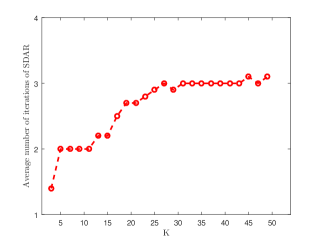
Figure 2: The average number of iterations of SDAR as $K$ increases.

We also have the option to stop the iteration early according to other criterions. For example, we can run SDAR (Algorithm 1) by gradually increasing $T$ until the change in the consecutive solutions is smaller than a given value. Candès, Romberg and Tao (2006) proposed to recover $\mathbf{\beta}^{*}$ based on (3.13) by finding the most sparse solution whose residual sum of squares is smaller than a prespecified noise level $\varepsilon$. Inspired by this, we can also run SDAR by increasing $T$ gradually until the residual sum of squares is smaller than a prespecified value $\varepsilon$.

We summarize these ideas in Algorithm 2 (Adaptive SDAR Algorithm) below.

Algorithm 2 Adaptive SDAR (ASDAR)

0:  Initial guess $\beta^{0},d^{0}$, an integer $\tau$, an integer $L$, and an early stopping criterion (optional). Set $k=1$.

1:  for $k=1,2,\cdots$ do

2:     Run Algorithm 1 with $T=\tau k$ and with initial value $(\beta^{k-1},d^{k-1})$. Denote the output by $(\beta^{k},d^{k})$.

3:     if the early stopping criterion is satisfied or $T>L$ then

4:        stop

5:     else

6:        $k=k+1$.

7:     end if

8:  end for

8:  $\hat{\beta}(\hat{T})$ as estimations of $\beta^{*}$.

5 Computational complexity

We look at the number of floating point operations line by line in Algorithm 1. Clearly it takes $O(p)$ flops to finish step 2-4. In step 5, we use conjugate gradient (CG) method (Golub and Van Loan, 2012) to solve the linear equation iteratively. During CG iterations the main operation is two matrix-vector multiplications which cost $2n|A_{k+1}|$ flops (the term $X^{\prime}y$ on the right-hand side can be precomputed and stored). Therefore we can control the number of CG iterations smaller than $p/(2|A_{k+1}|)$ to ensure that $O(np)$ flops will be enough for step 5. In step 6, calculating the matrix-vector product costs $np$ flops. As for step 7, checking the stop condition needs $O(p)$ flops. So the the overall cost per iteration of Algorithm 1 is $O(np)$. By Corollary 3.2 it needs no more than $O(\log(R))$ iterations to get a good solution for Algorithm 1 under the certain conditions. Therefore the overall cost of Algorithm 1 is $O(np\log(R))$ for exactly sparse and approximately sparse case under proper conditions.

Now we consider the cost of ASDAR (Algorithm 2). Assume ASDAR is stopped when $k=L$. Then the above discussion shows the the overall cost of Algorithm 2 is bounded by $O(Lnp\log(R))$ which is very efficient for large scale high dimension problem since the cost increases linearly in the ambient dimension $p$.

6 Comparison with greedy and screening methods

We give a high level comparison between SDAR and several greedy and screening methods, including OMP [Mallat and Zhang (1993), Tropp (2004), Donoho, Elad and Temlyakov (2006), Cai and Wang (2011), Zhang (2011a)], FoBa [Zhang 2011b)], GraDes [Garg and Khandekar (2009)], and SIS [Fan and Lv (2008)]. These greedy methods iteratively select/remove one or more variables and project the response vector onto the linear subspace spanned by the variables that have already been selected. From this point of view, they and SDAR share a similar characteristic. However, OMP and FoBa, select one variable per iteration based on the current correlation, i.e., the dual variable $d^{k}$ in our notation, while SDAR selects $T$ variables at a time based on the sum of primal ($\mathbf{\beta}^{k}$) and dual ($d^{k}$) information. The following interpretation in a low-dimensional setting with a small noise term may clarify the differences between these two approaches. If $X^{\prime}X/n\approx\textbf{E}$ and $\eta\approx\textrm{0}$, we have

$$d^{k}=X^{\prime}(y-X\mathbf{\beta}^{k})/n=X^{\prime}(X\mathbf{\beta}^{*}+\eta-X\mathbf{\beta}^{k})/n\approx\beta^{*}-\mathbf{\beta}^{k}+X^{\prime}\eta/n\approx\beta^{*}-\mathbf{\beta}^{k},$$

and

$$\mathbf{\beta}^{k}+d^{k}\approx\beta^{*}.$$

Hence, SDAR can approximate the underlying support $A^{*}$ more accurately than OMP and Foba. This is supported by the simulation results given in Section 6. GraDes can be formulated as

$$\beta^{k+1}=H_{K}(\beta^{k}+s_{k}d^{k}),$$ (6.1)

where $H_{K}(\cdot)$ is the hard thresholding operator by keeping the first $K$ largest elements and setting others to $0$, $s_{k}$ is the step size of gradient descent. Specifically, GraDes uses $s_{k}=1/(1+\delta_{2K})$, where $\delta_{2K}$ is the RIP constant. Intuitively, GraDes works by reducing the squares loss with gradient descent with different step sizes and preserving sparsity using hard thresholding. Hence, GraDes uses both primal and dual information to detect the support of the solution, which is similar to SDAR. However, after the approximate active set is determined, SDAR does a least-square fitting, which is more efficient and more accurate than just keeping the largest elements by hard thresholding. This is also supported by the simulation results given in Section 6.

Fan and Lv (2008) proposed SIS for dimension reduction in ultrahigh dimensional liner regression problems. This method selects variables with the $T$ largest absolute values of $X^{\prime}y$. To improve the performance of SIS, Fan and Lv (2008) also considered an iterative SIS, which iteratively selects more than one feature at a time until a desired number of variables are selected. They reported that the iterative SIS outperforms SIS numerically. However, the iterative SIS lacks a theoretically analysis. Interestingly, the first step in SDAR initialized with 0 is exactly the same as the SIS. But again the process of SDAR is different from the iterative SIS in that the active set of SDAR is determined based on the sum of primal and dual approximations while the iterative SIS uses dual only.

7 Simulation Studies

7.1 Implementation

We implemented SDAR/ASDAR, FoBa, GraDes and MCP in MatLab. For FoBa, our MatLab implementation follows the R package developed by Zhang (2011a). We optimize it by keeping track of rank-one updates after each greedy step. Our implementation of MCP uses the iterative threshholding algorithm (She, 2009) with warm start. The publicly available Matlab packages for LARS (included in the SparseLab package) are used. Since LARS and FoBa add one variable at a time, we stop them when $K$ variables are selected in addition to their default stopping conditions. (Of course, by doing this it will speed up and get better solutions for these three solvers).

In GraDes, the optimal gradient step length $s_{k}$ depends on the RIP constant of $X$, which is NP hard to compute [Tillmann and Pfetsch (2014)]. Here, we set $s_{k}=1/3$ following Garg and Khandekar (2009). We stop GraDes when the residual norm is smaller than $\varepsilon=\sqrt{n}\sigma$, or the maximum number of iterations is greater than $n/2$. We compute the MCP solution path and select an optimal solution using the HBIC [Wang, Kim and Li (2013)]. We stop the iteration when the residual norm is smaller than $\varepsilon={\|\eta\|}_{2}$, or the estimated support size is greater than $L=n/\log(n)$. In ASDAR (Algorithm 2), we set $\tau=50$ and we stop the iteration if the residual $\|y-X\beta^{k}\|$ is smaller than $\varepsilon=\sqrt{n}\sigma$ or $k\geq L=n/\log(n)$.

7.2 Accuracy and efficiency

We compare the accuracy and efficiency of SDAR/ASDAR with Lasso (LARS), MCP, GraDes and FoBa.

We first generate an $n\times p$ random Gaussian matrix $\bar{X}$ whose entries are i.i.d. $\sim\mathcal{N}(0,1)$ and then normalize its columns to the $\sqrt{n}$ length. Then the design matrix $X$ is generated with $X_{1}=\bar{X}_{1}$ and $X_{j}=\bar{X}_{j}+\rho(\bar{X}_{j+1}+\bar{X}_{j-1}),j=2,\ldots,p-1$. The underlying regression coefficient $\mathbf{\beta}^{*}$ is generated with the nonzero coefficients uniformly distributed in $[m,M]$, where $m=\sigma\sqrt{2\log(p)/n}$ and $M=100m$. Then the observation vector $y=X\beta^{*}+\eta$ with $\eta_{i}\thicksim\mathcal{N}(0,\sigma^{2})$, $i=1,\ldots,n$.

We consider a moderately large scale setting with $n=5000$ and $p=50000$. The number of nonzero coefficients is set to be $K=400$. So the sample size $n$ is about $O(K\log(p-K))$, which is nearly at the limit of estimating $\mathbf{\beta}^{*}$ in the linear model (1.1) by the Lasso with theoretically guaranteed [Wainwright (2009)]. The data are generated from the model described above with $K=400,R=100$. We set $\sigma=1$ and $\rho=0.2,0.4$ and $0.6$.

Table 1 shows the results based on $100$ independent replications. The first column gives the correlation value $\rho$ and the second column shows the methods in the comparison. The third to fifth columns give the averaged CPU time (in seconds), the averaged relative error defined as ($\textrm{ReErr}=\sum\|\hat{\beta}-\beta^{*}\|/\|\beta^{*}\|$), respectively, where $\hat{\beta}$ denotes the estimates and $\hat{A}=\textrm{supp}(\hat{\beta})$. The standard deviations of the CPU times and the relative errors are shown in the parentheses. In each column of the Table 1, the results in boldface indicate the best performers.

Table 1: Numerical results (CPU time, relative errors) on data set with $n=5000,p=50000,K=400,R=100,\sigma=1,\rho=0.2:0.2:0.6$.

$\rho$	method	ReErr	time(s)
	LARS	1.1e-1 (2.5e-2)	4.8e+1 (9.8e-1)
	MCP	7.5e-4 (3.6e-5)	9.3e+2 (2.4e+3)
$0.2$	GraDes	1.1e-3 (7.0e-5)	2.3e+1 (9.0e-1)
	FoBa	7.5e-4 (7.0e-5)	4.9e+1 (3.9e-1)
	ASDAR	7.5e-4 (4.0e-5)	8.4e+0 (4.5e-1)
	SDAR	7.5e-4 (4.0e-5)	1.4e+0 (5.1e-2)
	LARS	1.8e-1 (1.2e-2)	4.8e+1 (1.8e-1)
	MCP	6.2e-4 (3.6e-5)	2.2e+2 (1.6e+1)
$0.4$	GraDes	8.8e-4 (5.7e-5)	8.7e+2 (2.6e+3)
	FoBa	1.0e-2 (1.4e-2)	5.0e+1 (4.2e-1)
	ASDAR	6.0e-4 (2.6e-5)	8.8e+0 (3.2e-1)
	SDAR	6.0e-4 (2.6e-5)	2.3e+0 (1.7e+0)
	LARS	3.0e-1 (2.5e-2)	4.8e+1 (3.5e-1)
	MCP	4.5e-4 (2.5e-5)	4.6e+2 (5.1e+2)
$0.6$	GraDes	7.8e-4 (1.1e-4)	1.5e+2 (2.3e+2)
	FoBa	8.3e-3 (1.3e-2)	5.1e+1 (1.1e+0)
	ASDAR	4.3e-4 (3.0e-5)	1.1e+1 (5.1e-1)
	SDAR	4.3e-4 (3.0e-5)	2.1e+0 (8.6e-2)

We see that when the correlation $\rho$ is low, i.e., $\rho=0.2$, MCP, FoBa, SDAR and ASDAR are on the top of the list in average error (ReErr). In terms of speed, SDAR/ASDAR is almost 20-900/3-100 times faster than the other methods. As the correlation $\rho$ increases to $\rho=0.4$ and $\rho=0.6$, FoBa becomes less accurate than SDAR/ASDAR. The accuracy of MCP is similar to that of SDAR/ASDAR, but MCP is 20 to 100 times slower than SDAR/ASDAR. The standard deviations of the CPU times and the relative errors of MCP and SDAR/ASDAR are similar and smaller than those of the other methods in all the three settings.

7.3 Influence of the model parameters

We now consider the effects of each of the model parameters on the performance of ASDAR, LARS, MCP, GraDes and FoBa more closely.

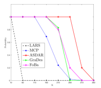
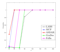
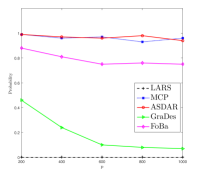
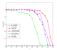
Figure 3: Numerical results of the influence of sparsity level $K$ (top left panel), sample size $n$ (top right panel), ambient dimension $p$ (bottom left panel) and correlation $\rho$ (bottom right panel) on the probability of exact recovery of the true support of all the solvers considered here.

In this set of simulations, the rows of the design matrix $X$ are drawn independently from $\mathcal{N}(0,\Sigma)$ with $\Sigma_{jk}=\rho^{|j-k|},1\leq j,k\leq p$. The elements of the error vector $\eta$ are generated independently with $\eta_{i}\thicksim\mathcal{N}(0,\sigma^{2})$, $i=1,\ldots,n$. Let $R=M/m$, where, $M=\max\{|\beta^{*}_{A^{*}}|\},m=\min\{|\beta^{*}_{A^{*}}|\}=1$. The underling regression coefficient vector $\beta^{*}\in\mathbb{R}^{p}$ is generated in such a way that $A^{*}$ is a randomly chosen subset of $\{1,2,...,p\}$ with $|A^{*}|=K<n$ and $R\in[1,10^{3}]$. Then the observation vector $y=X\beta^{*}+\eta$. We use $\{n,p,K,\sigma,\rho,R\}$ to indicate the parameters used in the data generating model described above.

We run ASDAR with $\tau=5,L=n/\log(n)$ (if not specified). We use the HBIC [Wang, Kim and Li (2013)] to select the tuning parameter $T$. The simulation results given in Figure 3 are based on 100 independent replications.

7.3.1 Influence of the sparsity level $K$

The top left panel of Figure 3 shows the results of the influence of sparsity level $K$ on the probability of exact recovery of $A^{*}$ of ASDAR, LARS, MCP, GraDes and FoBa on data sets with $(n=500,p=1000,K=10:50:360,\sigma=0.5,\rho=0.1,R=10^{3})$. Here $10:50:360$ means the sample size starts from 10 to 360 with an increment of 50. We use $L=0.8n$ for both ASDAR and MCP to eliminate the effect of stopping rule since the maximum $K=360$. When the sparsity level $K=10$, all the solvers performed well in recovering the true support. As $K$ increases, LARS was the first one that failed to recover the support and vanished when $K=60$ (this phenomenon had also been observed in Garg and Khandekar (2009)), MCP began to fail when $K>110$, GraDes and FoBa began to fail when $K>160$. In comparison, ASDAR was still able to do well even when $K=260$.

7.3.2 Influence of the sample size $n$

The top right panel of Figure 3 shows the influence of the sample size $n$ on the probability of correctly estimating $A^{*}$ with data generated from the model with $(n=30:20:200,p=500,K=10,\sigma=0.1,\rho=0.1,R=10)$. We see that the performances of all the five methods become better as $n$ increases. However, ASDAR performs better than the others when $n=30$ and $50$.

7.3.3 Influence of the ambient dimension $p$

The bottom left panel of Figure 3 shows the influence of ambient dimension $p$ on the performance of ASDAR, LARS, MCP, GraDes and FoBa on data with $(n=100,p=200:200:1000,K=20,\sigma=1,\rho=0.3,R=10)$. We see that the probabilities of exactly recovering the support of the underlying coefficients of ASDAR and MCP are higher than those of the other solvers as $p$ increasing, which indicate that ASDAR and MCP are more robust to the ambient dimension.

7.3.4 Influence of correlation $\rho$

The bottom right panel of Figure 3 shows the influence of correlation $\rho$ on the performance of ASDAR, LARS, MCP, GraDes and FoBa on data with $(n=150,p=500,K=25,\sigma=0.1,\rho=0.05:0.1:0.95,R=10^{2})$. We see that the performance of all the solvers become worse when the correlation $\rho$ increasing. However, ASDAR generally performed better than the other methods as $\rho$ increases.

In summary, our simulation studies demonstrate that SDAR/ASDAR is generally more accurate, more efficient and more stable than Lasso, MCP, FoBa and GraDes.

8 Concluding remarks

SDAR is a constructive approach for fitting sparse, high-dimensional linear regression models. Under appropriate conditions, we established the nonasymptotic minimax $\ell_{2}$ error bound and optimal $\ell_{\infty}$ error bound of the solution sequence generated by SDAR. We also calculated the number of iterations required to achieve these bounds. In particular, an interesting and surprising aspect of our results is, if a mutual coherence condition on the design matrix is satisfied, the number of iterations required for the SDAR to achieve the optimal $\ell_{\infty}$ bound does not depend on the underlying sparsity level. In addition, SDAR has the same computational complexity per iteration as LARS, coordinate descent and greedy methods. SDAR/ ASDAR is accurate, fast, stable and easy to implement. Our simulation studies demonstrate that SDAR/ ASDAR is competitive with or outperforms the Lasso, MCP and several greedy methods in efficiency and accuracy. These theoretical and numerical results suggest that SDAR/ ASDAR is a promising alternative to the existing penalized and greedy methods for dealing with large scale high-dimensional linear regression problems.

We have only considered the linear regression model. It would be interesting to generalize SDAR to other models with more general loss functions or models with other types of sparsity structures. It would also be interesting to develop parallel or distributed versions of SDAR that can run on multiple cores for data sets with big $n$ and large $p$ or when data are distributively stored.

We have implemented SDAR in a Matlab package sdar, which is available at http://homepage.stat.uiowa.edu/~jian/.

9 Appendix: Proofs

Proof of Lemma 2.1. Let $L_{\lambda}(\beta)=\frac{1}{2n}{\|X\mathbf{\beta}-y\|}_{2}^{2}+\lambda{\|\mathbf{\beta}\|}_{0}.$ Suppose $\beta^{\diamond}$ is a minimizer of $L_{\lambda}$. Then

$$\beta_{i}^{\diamond}\in\mathop{\textrm{missing}}{argmin}\limits_{t\in\mathbb{R}}L_{\lambda}(\beta_{1}^{\diamond},...,\beta_{i-1}^{\diamond},t,\beta_{i+1}^{\diamond},...,\beta_{p}^{\diamond})$$

$$\Rightarrow \beta_{i}^{\diamond}\in\mathop{\textrm{missing}}{argmin}\limits_{t\in\mathbb{R}}\tfrac{1}{2n}{\|X\beta^{\diamond}-y+(t-\beta_{i}^{\diamond})X_{i}\|}_{2}^{2}+\lambda|t|_{0}$$

$$\Rightarrow \beta_{i}^{\diamond}\in\mathop{\textrm{missing}}{argmin}\limits_{t\in\mathbb{R}}\tfrac{1}{2}(t-\beta_{i}^{\diamond})^{2}+\tfrac{1}{n}(t-\beta_{i}^{\diamond})X_{i}^{\prime}(X\beta^{\diamond}-y)+\lambda|t|_{0}$$

$$\Rightarrow \beta_{i}^{\diamond}\in\mathop{\textrm{missing}}{argmin}\limits_{t\in\mathbb{R}}\tfrac{1}{2}(t-(\beta_{i}^{\diamond}+X_{i}^{\prime}(y-X\beta^{\diamond})/n))^{2}+\lambda|t|_{0}.$$

Let $d^{\diamond}=X^{\prime}(y-X\beta^{\diamond})/n$. By the definition of the hard thresholding operator $H_{\lambda}(\cdot)$ in (2.3), we have

$$\beta^{\diamond}_{i}=H_{\lambda}(\beta^{\diamond}_{i}+d^{\diamond}_{i})\quad\mbox{ for }i=1,...,p,$$

which shows (2.2) holds.

Conversely, suppose (2.2) holds. Let

$$A^{\diamond}=\Big{\{}i\in S\big{|}\left|\beta^{\diamond}_{i}+d^{\diamond}_{i}\right|\geq\sqrt{2\lambda}\Big{\}}.$$

By (2.2) and the definition of $H_{\lambda}(\cdot)$ in (2.3), we deduce that for $i\in A^{\diamond}$, $|\beta_{i}^{\diamond}|\geq\sqrt{2\lambda}$. Furthermore, $\textbf{0}=d^{\diamond}_{A^{\diamond}}=X_{A^{\diamond}}^{\prime}(y-X_{A^{\diamond}}\beta^{\diamond}_{A^{\diamond}})/n$, which is equivalent to

$$\beta^{\diamond}_{A^{\diamond}}\in\mathop{\textrm{missing}}{argmin}\tfrac{1}{2n}{\|X_{A^{\diamond}}\beta_{A^{\diamond}}-y\|}_{2}^{2}.$$ (9.1)

Next we show $L_{\lambda}(\beta^{\diamond}+h)\geq L_{\lambda}(\beta^{\diamond})$ if $h$ is small enough with ${\|h\|}_{\infty}<\sqrt{2\lambda}$. Two cases should be considered. If $h_{(A^{\diamond})^{c}}\neq 0$, then

$$L_{\lambda}(\beta^{\diamond}+h)-L_{\lambda}(\beta^{\diamond}) \geq\tfrac{1}{2n}{\|X\beta^{\diamond}-y+Xh\|}_{2}^{2}-\tfrac{1}{2n}{\|X\beta^{\diamond}-y\|}_{2}^{2}+\lambda\geq\lambda-|\langle h,d^{\diamond}\rangle|,$$

which is positive for sufficiently small $h$. If $h_{(A^{\diamond})^{c}}=0$, by the minimizing property of $\beta^{\diamond}_{A^{\diamond}}$ in (9.1) we deduce $L_{\lambda}(\beta^{\diamond}+h)\geq L_{\lambda}(\beta^{\diamond})$. This completes the proof of Lemma 2.1. $\hfill\Box$

Lemma 9.1.

Let $A$, $B$ be disjoint subsets of $S$, with $\left|A\right|=a$, $\left|B\right|=b$. Assume $X\sim\textrm{SRC}(c_{-}(a+b),c_{+}(a+b),a+b)$. Let $\theta_{a,b}$ be the sparse orthogonality constant and let $\mu$ be the mutual coherence of $X$. Then we have

$$nc_{-}(a)\leq\left\|X_{A}^{T}X_{A}\right\|\leq nc_{+}(a),$$ (9.2)

$$\frac{1}{nc_{+}(a)}\leq\left\|(X_{A}^{T}X_{A})^{-1}\right\|\leq\frac{1}{nc_{-}(a)},$$ (9.3)

$$\left\|X_{A}^{\prime}\right\|\leq\sqrt{nc_{+}(a)}$$ (9.4)

$$\theta_{a,b}\leq(c_{+}(a+b)-1)\vee(1-c_{-}(a+b))$$ (9.5)

$${\|X_{B}^{\prime}X_{A}u\|}_{\infty}\leq na\mu{\|u\|}_{\infty},\quad\forall u\in\mathbb{R}^{\left|A\right|},$$ (9.6)

$$\left\|X_{A}\right\|=\left\|X^{\prime}_{A}\right\|\leq\sqrt{n(1+(a-1)\mu)}.$$ (9.7)

Furthermore, if $\mu<1/(a-1)$, then

$${\|(X_{A}^{\prime}X_{A})^{-1}u\|}_{\infty}\leq\frac{{\|u\|}_{\infty}}{n(1-(a-1)\mu)},\quad\forall u\in\mathbb{R}^{\left|A\right|}.$$ (9.8)

Moreover, $c_{+}(s)$ is an increasing function of $s$, $c_{-}(s)$ a decreasing function of $s$ and $\theta_{a,b}$ an increasing function of $a$ and $b$.

Proof of Lemma 9.1. The assumption $X\sim\textrm{SRC}(a,c_{-}(a),c_{+}(a))$ implies the spectrum of $X_{A}^{\prime}X_{A}/n$ is contained in $[c_{-}(a),c_{+}(a)]$. So (9.2) - (9.4) hold. Let E be an $(a+b)\times(a+b)$ identity matrix. (9.5) follows from the fact that $X_{A}^{\prime}X_{B}/n$ is a submatrix of $X_{A\cup B}^{\prime}X_{A\cup B}/n-\textbf{E}$ whose spectrum norm is less than $(1-c_{-}(a+b))\vee(c_{+}(a+b)-1)$. Let $G=X^{\prime}X/n$. Then, $|\sum_{j=1}^{a}G_{i,j}u_{j}|\leq\mu a{\|u\|}_{\infty},$ for all $i\in B$, which implies (9.6). By Gerschgorin’s disk theorem,

$$|\left\|G_{A,A}\right\|-G_{i,i}|\leq\sum_{i\neq j=1}^{a}|G_{i,j}|\leq(a-1)\mu\quad\forall i\in A,$$

thus (9.7) holds. For (9.8), it suffices to show ${\|G_{A,A}u\|}_{\infty}\geq(1-(a-1)\mu){\|u\|}_{\infty}$ if $\mu<1/(a-1)$. In fact, let $i\in A$ such that ${\|u\|}_{\infty}=\left|u_{i}\right|$, then

$${\|G_{A,A}u\|}_{\infty}\geq|\sum_{j=1}^{a}G_{i,j}u_{j}|\geq|u_{i}|-\sum_{i\neq j=1}^{a}\left|G_{i,j}\right||u_{j}|\geq{\|u\|}_{\infty}-\mu(a-1){\|u\|}_{\infty}.$$

The last assertion follows from their definitions. This completes the proof of Lemma 9.1. $\hfill\Box$

We now define some notation that will be useful in the proof of Theorems 3.1 and 3.2 given below. For any given integers $T$ and $J$ with $T\geq J$ and $F\subseteq S$ with $|F|=T-J$, let $A^{\circ}=A^{*}_{J}\cup F$ and $I^{\circ}=(A^{\circ})^{c}$. Let $\{A^{k}\}_{k}$ be the active sets generated by Algorithm 1. Define

$$E_{2}(A^{k})={\|\bar{\beta}^{*}|_{A^{*}_{J}\backslash A^{k}}\|}_{2}\ \mbox{ and }\ E_{\infty}(A^{k})={\|\bar{\beta}^{*}|_{A^{*}\backslash A^{k}}\|}_{\infty}.$$

Let

$$A^{k}_{1}=A^{k}\cap A^{\circ},A^{k}_{2}=A^{\circ}\backslash A^{k}_{1},I^{k}_{3}=A^{k}\cap I^{\circ},I^{k}_{4}=I^{\circ}\backslash I^{k}_{3}.$$

Denote the cardinality of $I^{k}_{3}$ by $l_{k}=|I^{k}_{3}|$. Let

$$A^{k}_{11}=A^{k}_{1}\backslash(A^{k+1}\cap A^{k}_{1}),A^{k}_{22}=A^{k}_{2}\backslash(A^{k+1}\cap A^{k}_{2}),I^{k}_{33}=A^{k+1}\cap I^{k}_{3},I^{k}_{44}=A^{k+1}\cap I^{k}_{4},$$

and

$$\triangle^{k}=\mathbf{\beta}^{k+1}-\bar{\beta}^{*}|_{A^{k}}.$$

These notation can be easily understood in the case $T=J$. For example, $E_{2}(A^{k})$ ($E_{\infty}(A^{k})$) is a measure of the difference between the detected active set $A^{k}$ and the target support $A^{*}_{J}$. $A^{k}_{1}$ and $I^{k}_{3}$ contain the correct indexes and incorrect indexes in $A^{k}$, respectively. $A^{k}_{11}$ and $A^{k}_{22}$ include the indexes in $A^{\circ}$ that will be lost from the $k$th to $(k+1)$th iteration. $I^{k}_{33}$ and $I^{k}_{44}$ contain the indexes included in $I^{\circ}$ that will be gained. By Algorithm 1, we have $|A^{k}|=|A^{k+1}|=T$, $A^{k}=A^{k}_{1}\cup I^{k}_{3},$ $|A^{k}_{2}|=|A^{\circ}|-|A^{k}_{1}|=|A^{\circ}|-|I^{k}_{3}|=T-(T-l_{k})=l_{k}\leq T$, and

$$|A^{k}_{11}|+|A^{k}_{22}| =|I^{k}_{33}|+|I^{k}_{44}|,$$ (9.9)

$$E_{2}(A^{k}) ={\|\bar{\beta}^{*}|_{A^{\circ}\backslash A^{k}}\|}_{2}={\|\bar{\beta}^{*}|_{A^{k}_{2}}\|}_{2},$$ (9.10)

$$E_{\infty}(A^{k}) ={\|\bar{\beta}^{*}|_{A^{\circ}\backslash A^{k}}\|}_{\infty}={\|\bar{\beta}^{*}|_{A^{k}_{2}}\|}_{\infty}.$$ (9.11)

Before we give the technical proofs of Theorems and Corollaries we give description of of the main ideas behind the proofs. Intuitively, SDAR is a support detection and least square fitting process. Therefore our proofs justify the active sets $\{A^{k}\}_{k}$ generated by Algorithm 1 can approximate $A^{*}_{J}$ more and more accurately by showing that $E_{2}(A^{k}),E_{\infty}(A^{k})$ decays geometrically and the effect of the noise $\bar{\eta}$ can be well controlled with high probability. To this end, we need the following technical Lemmas 9.3 - 9.8. Lemma 9.3 shows the effect of noise $h_{2}(T)$ and $h_{\infty}(T)$ can be controlled by the sum of unrecoverable energy $R_{J}$ and the universal noise level $O(\sigma\sqrt{2\log(p)/n})$ with high probability if $\eta$ is sub-Gaussian. Lemma 9.4 shows the norm of both $\triangle^{k}$ and $\mathbf{\beta}^{k}-\bar{\beta}^{*}$ are mainly bounded by $E_{2}(A^{k})$ and $h_{2}(T)$ ($E_{\infty}(A^{k})$ and $h_{\infty}(T)$). Lemma 9.5 shows that $E_{2}(A^{k+1})$ ($E_{\infty}(A^{k+1})$) can be bounded by the norm of $\bar{\beta}^{*}$ on the lost indexes and further can be mainly controlled in terms of $E_{2}(A^{k})$, $h_{2}(T)$ ($E_{\infty}(A^{k})$, $h_{\infty}(T)$) and the norm of $\triangle^{k}$, $\mathbf{\beta}^{k+1}$ and $d^{k+1}$ on the lost indexes. Lemma 9.6 gives the benefits brought by the orthogonality of $\mathbf{\beta}^{k}$ and $d^{k}$ that the norm of $\mathbf{\beta}^{k+1}$ and $d^{k+1}$ on the lost indexes can be bounded by the norm on the gained indexes. Lemma 9.7 gives the upper bound of the norm of $\mathbf{\beta}^{k+1}+d^{k+1}$ on the gained indexes by the sum of $E_{2}(A^{k})$, $h_{2}(T)$ ($E_{\infty}(A^{k})$, $h_{\infty}(T)$), and the norm of $\triangle^{k}$. Then Lemma 9.8 get the desired relations of $E_{2}(A^{k+1})$ and $E_{2}(A^{k})$ ($E_{\infty}(A^{k+1})$ and $E_{\infty}(A^{k})$) by combining Lemma 9.3 - 9.7.

Lemma 9.2.

Suppose (A3) holds. We have for any $\alpha\in(0,1/2)$

$$\mathbf{P}\Big{(}{\|X^{\prime}\eta\|}_{\infty}\leq\sigma\sqrt{2\log(p/\alpha)n}\Big{)}\geq 1-2\alpha$$ (9.12)

$$\mathbf{P}\Big{(}\max_{|A|\leq T}{\|X_{A}^{\prime}\eta\|}_{2}\leq\sigma\sqrt{T}\sqrt{2\log(p/\alpha)n}\Big{)}\geq 1-2\alpha.$$ (9.13)

Proof of Lemma 9.2. This lemma follows from the sub-Gaussian assumption (A3) and standard probability calculation, see Candès and Tao (2007), Zhang and Huang (2008), Wainwright (2009) for a detail. $\hfill\Box$

Lemma 9.3.

Let $A\subset S$ with $|A|\leq T$. Suppose (A1) and (A3) holds. Then for $\alpha\in(0,1/2)$ with probability at least $1-2\alpha$, we have

• If $X\sim SRC(T,c_{-}(T),c_{+}(T))$, then

  $$h_{2}(T)\leq\varepsilon_{1}.$$ (9.14)

• $$h_{\infty}(T)\leq\varepsilon_{2}.$$ (9.15)

Proof.

We first show

$${\|X\mathbf{\beta}^{*}|_{(A^{*}_{J})^{c}}\|}_{2}\leq\sqrt{nc_{+}(J)}R_{J},$$ (9.16)

under the assumption of $X\sim SRC(c_{-}(T),c_{+}(T),T)$ and (A1). In fact, let $\beta$ be an arbitrary vector in $\mathbb{R}^{p}$ and $A_{1}$ be the first $J$ largest positions of $\beta$, $A_{2}$ be the next and so forth. Then

$${\|X\beta\|}_{2} \leq{\|X\beta_{A_{1}}\|}_{2}+\sum_{i\geq 2}{\|X\beta_{A_{i}}\|}_{2}$$

$$\leq\sqrt{nc_{+}(J)}{\|\beta_{A_{1}}\|}_{2}+\sqrt{nc_{+}(J)}\sum_{i\geq 2}{\|\beta_{A_{i}}\|}_{2}$$

$$\leq\sqrt{nc_{+}(J)}{\|\beta\|}_{2}+\sqrt{nc_{+}(J)}\sum_{i\geq 1}\sqrt{\frac{1}{J}}{\|\beta_{A_{i-1}}\|}_{1}$$

$$\leq\sqrt{nc_{+}(J)}({\|\beta\|}_{2}+\sqrt{\frac{1}{J}}{\|\beta\|}_{1}),$$

where the first inequality uses the triangle inequality, the second inequality uses (9.4), and the third and fourth ones are simple algebra. This implies (9.16) holds by observing the definition of $R_{J}$. By the triangle inequality, (9.4), (9.16) and (9.13), we have with probability at least $1-2\alpha$,

$${\|X_{A}^{\prime}\bar{\eta}\|}_{2}/n \leq{\|X^{\prime}_{A}X\mathbf{\beta}^{*}|_{(A^{*}_{J})^{c}}\|}_{2}/n+{\|X^{\prime}_{A}\eta\|}_{2}/n$$

$$\leq c_{+}(J)R_{J}+\sigma\sqrt{T}\sqrt{2\log(p/\alpha)/n},$$

Therefore, (9.14) follows by noticing the monotone increasing property of $c_{+}(\cdot)$, the definition of $\varepsilon_{1}$ and the arbitrariness of $A$.

Repeating the proof process of (9.17) and replacing $\sqrt{nc_{+}(J)}$ with $\sqrt{n(1+(J-1)\mu)}$ by using (9.7) we get

$${\|X\mathbf{\beta}^{*}|_{(A^{*}_{J})^{c}}\|}_{2}\leq\sqrt{n(1+(K-1)\mu)}R_{J}.$$ (9.17)

Therefore, by (9.7), (9.17) and (9.12), we have with probability at least $1-2\alpha$,

$${\|X_{A}^{\prime}\bar{\eta}\|}_{\infty}/n \leq{\|X_{A}^{\prime}X\mathbf{\beta}^{*}|_{(A^{*}_{J})^{c}}\|}_{\infty}/n+{\|X^{\prime}_{A}\eta\|}_{2}/n$$

$$\leq{\|X_{A}^{\prime}X\mathbf{\beta}^{*}|_{(A^{*}_{J})^{c}}\|}_{2}/n+{\|X^{\prime}_{A}\eta\|}_{2}/n$$

$$\leq(1+(J-1)\mu)R_{J}+\sigma\sqrt{2\log(p/\alpha)/n}.$$

This implies part (ii) of Lemma 9.3 by noticing the definition of $\varepsilon_{2}$ and the arbitrariness of $A$. ∎

Lemma 9.4.

Let $A\subset S$ with $|A|\leq T$. Suppose (A1) holds.

• If $X\sim\textrm{SRC}(T,c_{-}(T),c_{+}(T))$,

  $${\|\mathbf{\beta}^{k+1}-\bar{\beta}^{*}\|}_{2}\leq\Big{(}1+\frac{\theta_{T,T}}{c_{-}(T)}\Big{)}E_{2}(A^{k})+\frac{h_{2}(T)}{c_{-}(T)},$$ (9.18)

• If $(T-1)\mu<1$, then

  $${\|\mathbf{\beta}^{k+1}-\bar{\beta}^{*}\|}_{\infty}\leq\frac{1+\mu}{1-(T-1)\mu}E_{\infty}(A^{k})+\frac{h_{\infty}(T)}{1-(T-1)\mu}.$$ (9.19)

Proof.

$$\mathbf{\beta}^{k+1}_{A^{k}} =(X_{A^{k}}^{\prime}X_{A^{k}})^{-1}X_{A^{k}}^{\prime}y$$

$$=(X_{A^{k}}^{\prime}X_{A^{k}})^{-1}X_{A^{k}}^{\prime}(X_{A^{k}_{1}}\bar{\beta}^{*}_{A^{k}_{1}}+X_{A^{k}_{2}}\bar{\beta}^{*}_{A^{k}_{2}}+\bar{\eta}),$$ (9.20)

$$(\bar{\beta}^{*}|_{A^{k}})_{A^{k}} =(X_{A^{k}}^{\prime}X_{A^{k}})^{-1}X_{A^{k}}^{\prime}X_{A^{k}}(\bar{\beta}^{*}|_{A^{k}})_{A^{k}}$$

$$=(X_{A^{k}}^{\prime}X_{A^{k}})^{-1}X_{A^{k}}^{\prime}(X_{A^{k}_{1}}\bar{\beta}^{*}_{A^{k}_{1}})$$ (9.21)

where the first equality uses the definition of $\mathbf{\beta}^{k+1}$ in Algorithm 1, the second equality uses $y=X\bar{\beta}^{*}+\bar{\eta}=X_{A^{k}_{1}}\bar{\beta}^{*}_{A^{k}_{1}}+X_{A^{k}_{2}}\bar{\beta}^{*}_{A^{k}_{2}}+\bar{\eta}$, the third equality is simple algebra, and the last one uses the definition of $A^{k}_{1}.$

$${\|\triangle^{k}\|}_{2} ={\|\mathbf{\beta}^{k+1}_{A^{k}}-(\bar{\beta}^{*}|_{A^{k}})_{A^{k}}\|}_{2}$$

$$={\|(X_{A^{k}}^{\prime}X_{A^{k}})^{-1}X_{A^{k}}^{\prime}(X_{A^{k}_{2}}\bar{\beta}^{*}_{A^{k}_{2}}+\bar{\eta})\|}_{2}$$

$$\leq\frac{1}{nc_{-}(T)}({\|X_{A^{k}}^{\prime}X_{A^{k}_{2}}\bar{\beta}^{*}_{A^{k}_{2}}\|}_{2}+{\|X_{A^{k}}^{\prime}\bar{\eta}\|}_{2})$$

$$\leq\frac{\theta_{T,T}}{c_{-}(T)}{\|\bar{\beta}^{*}|_{A^{k}_{2}}\|}_{2}+\frac{h_{2}(T)}{c_{-}(T)}$$ (9.22)

where the first equality uses $\textrm{supp}(\mathbf{\beta}^{k+1})=A^{k}$, the second equality uses (9.21) and (9.20), the first inequality uses (9.3) and the triangle inequality, and the second inequality uses (9.10), the definition of $\theta_{a,b}$ and $h_{2}(T)$. Then the triangle inequality ${\|\mathbf{\beta}^{k+1}-\bar{\beta}^{*}\|}_{2}\leq{\|\mathbf{\beta}^{k+1}-\bar{\beta}^{*}|_{A^{k}}\|}_{2}+{\|\bar{\beta}^{*}|_{A^{\circ}\backslash A^{k}}\|}_{2}$ and (9.22) imply (9.18).

Similar to the proof of (9.22) and using (9.8), (9.6), (9.11), we have

$${\|\triangle^{k}\|}_{\infty}\leq\frac{T\mu}{1-(T-1)\mu}{\|\bar{\beta}^{*}|_{A^{k}_{2}}\|}_{\infty}+\frac{h_{\infty}(T)}{(1-(T-1)\mu)}$$ (9.23)

Thus (9.19) follows by using triangle inequality and (9.23). This completes the proof of Lemma 9.4. ∎

Lemma 9.5.

$$E_{2}(A^{k+1}) \leq{\|\bar{\beta}^{*}_{A^{k}_{11}}\|}_{2}+{\|\bar{\beta}^{*}_{A^{k}_{22}}\|}_{2},$$ (9.24)

$$E_{\infty}(A^{k+1}) \leq{\|\bar{\beta}^{*}_{A^{k}_{11}}\|}_{\infty}+{\|\bar{\beta}^{*}_{A^{k}_{22}}\|}_{\infty}.$$ (9.25)

$${\|\bar{\beta}^{*}_{A^{k}_{11}}\|}_{2} \leq{\|\triangle^{k}_{A^{k}_{11}}\|}_{2}+{\|\mathbf{\beta}^{k+1}_{A^{k}_{11}}\|}_{2},$$ (9.26)

$${\|\bar{\beta}^{*}_{A^{k}_{11}}\|}_{\infty} \leq{\|\triangle^{k}_{A^{k}_{11}}\|}_{\infty}+{\|\mathbf{\beta}^{k+1}_{A^{k}_{11}}\|}_{\infty}.$$ (9.27)

Furthermore, assume (A1) holds. We have

$${\|\bar{\beta}^{*}_{A^{k}_{22}}\|}_{\infty} \leq{\|d^{k+1}_{A^{k}_{22}}\|}_{\infty}+T\mu{\|\triangle^{k}_{A^{k}}\|}_{\infty}+T\mu E_{\infty}(A^{k})+h_{\infty}(T)$$ (9.28)

$${\|\bar{\beta}^{*}_{A^{k}_{22}}\|}_{2} \leq\frac{{\|d^{k+1}_{A^{k}_{22}}\|}_{2}+\theta_{T,T}{\|\triangle^{k}_{A^{k}}\|}_{2}+\theta_{T,T}E_{2}(A^{k})+h_{2}(T)}{c_{-}(T)}\quad\textrm{ if}\quad X\sim\textrm{SRC}(c_{-}(T),c_{+}(T),T).$$ (9.29)

Proof.

$$E_{2}(A^{k+1})={\|\bar{\beta}^{*}|_{A^{\circ}\backslash A^{k+1}}\|}_{2}={\|\bar{\beta}^{*}|_{A^{k}_{11}\cup A^{k}_{22}}\|}_{2}\leq{\|\bar{\beta}^{*}_{A^{k}_{11}}\|}_{2}+{\|\bar{\beta}^{*}_{A^{k}_{22}}\|}_{2},$$

where the first and second equality use the diminution of $E_{2}(A^{k+1})$ and the definition of $A^{k}_{11}$, $A^{k}_{11}$, $A^{k}_{22}$, respectively. This proves (9.24). (9.25) can be proved similarly.

$${\|\mathbf{\beta}^{k+1}_{A^{k}_{11}}\|}_{2} ={\|\Big{(}\bar{\beta}^{*}\big{|}_{A^{k}}\Big{)}_{A^{k}_{11}}+\triangle^{k}_{A^{k}_{11}}\|}_{2}\geq{\|\bar{\beta}^{*}_{A^{k}_{11}}\|}_{2}-{\|\triangle^{k}_{A^{k}_{11}}\|}_{2}$$

where the equality uses the definition of $\triangle^{k}=\mathbf{\beta}^{k+1}-\bar{\beta}^{*}|_{A^{k}}$, the inequality is triangle inequality. This proves (9.26). (9.27) can be proved in the same way.

$${\|d^{k+1}_{A^{k}_{22}}\|}_{2} ={\|X_{A^{k}_{22}}^{\prime}\Big{(}X_{A^{k}}\mathbf{\beta}^{k+1}_{A^{k}}-y\Big{)}/n\|}_{2}$$

$$={\|X_{A^{k}_{22}}^{\prime}\Big{(}X_{A^{k}}\triangle^{k}_{A^{k}}+X_{A^{k}}\bar{\beta}^{*}_{A^{k}}-X_{A^{\circ}}\bar{\beta}^{*}_{A^{\circ}}-\bar{\eta}\Big{)}/n\|}_{2}$$

$$={\|X_{A^{k}_{22}}^{\prime}\Big{(}X_{A^{k}}\triangle^{k}_{A^{k}}-X_{A^{k}_{22}}\bar{\beta}^{*}_{A^{k}_{22}}-X_{A^{k}_{2}\backslash A^{k}_{22}}\bar{\beta}^{*}_{A^{k}_{2}\backslash A^{k}_{22}}-\bar{\eta}\Big{)}/n\|}_{2}$$

$$\geq c_{-}(|A^{k}_{22}|){\|\bar{\beta}^{*}_{A^{k}_{22}}\|}_{2}-\theta_{|A^{k}_{22}|,T}{\|\triangle^{k}_{A^{k}}\|}_{2}-\theta_{l_{k},l_{k}-|A^{k}_{22}|}{\|\bar{\beta}^{*}_{A^{k}_{2}\backslash A^{k}_{22}}\|}_{2}-{\|X_{A^{k}_{22}}\bar{\eta}/n\|}_{2}$$

$$\geq c_{-}(T){\|\bar{\beta}^{*}_{A^{k}_{22}}\|}_{2}-\theta_{T,T}{\|\triangle^{k}_{A^{k}}\|}_{2}-\theta_{T,T}E_{2}(A^{k})-h_{2}(T),$$

where the first equality uses the definition of $d^{k+1}$, the second equality uses the the definition of $\triangle^{k}$ and $y$, the third equality is simple algebra, the first inequality uses the triangle inequality, (9.2) and the definition of $\theta_{a,b}$, and the last inequality uses the monotonicity property of $c_{-}(\cdot)$, $\theta_{a,b}$ and the definition of $h_{2}(T)$. This proves (9.29).

Let $i_{k}\in A^{k}_{22}$ such that ${\|\bar{\beta}^{*}_{A^{k}_{22}}\|}_{\infty}=\left|\bar{\beta}^{*}_{i_{k}}\right|$.

$$\left|d^{k+1}_{i_{k}}\right| ={\|X_{i_{k}}^{\prime}(X_{A^{k}}\triangle^{k}_{A^{k}}-X_{i_{k}}\bar{\beta}^{*}_{i_{k}}-X_{A^{k}_{2}\backslash\ i_{k}}\bar{\beta}^{*}_{A^{k}_{2}\backslash\ i_{k}}-\bar{\eta})/n\|}_{\infty}$$

$$\geq\left|\bar{\beta}^{*}_{i_{k}}\right|-T\mu{\|\triangle^{k}_{A^{k}}\|}_{\infty}-l_{k}\mu{\|\bar{\beta}^{*}_{A^{k}_{2}\backslash\ i_{k}}\|}_{\infty}-{\|X_{i_{k}}^{\prime}\bar{\eta}\|}_{\infty}$$

$$\geq{\|\bar{\beta}^{*}_{A^{k}_{22}}\|}_{\infty}-T\mu{\|\triangle^{k}_{A^{k}}\|}_{\infty}-T\mu E_{\infty}(A^{k})-h_{\infty}(T),$$

where the first equality is derived from the first three equalities in the proof of (9.29) by replacing $A^{k}_{22}$ with $i_{k}$, the first inequality uses the triangle inequality and (9.6), and the last inequality uses the definition of $h_{\infty}(T)$. Then (9.28) follows by rearranging the terms in the above inequality. This completes the proof of Lemma 9.5. ∎

Lemma 9.6.

$${\|\mathbf{\beta}^{k}\|}_{\infty}\vee{\|d^{k}\|}_{\infty} =\max\{|\mathbf{\beta}^{k}_{i}|+|d^{k}_{i}|\big{|}i\in S\},\forall k\geq 1.$$ (9.30)

$${\|\mathbf{\beta}^{k+1}_{A^{k}_{11}}\|}_{\infty}+{\|d^{k+1}_{A^{k}_{22}}\|}_{\infty} \leq\left|\mathbf{\beta}^{k+1}_{I^{k}_{33}}\right|_{min}\wedge\left|d^{k+1}_{I^{k}_{44}}\right|_{min}.$$ (9.31)

$${\|\mathbf{\beta}^{k+1}_{A^{k}_{11}}\|}_{2}+{\|d^{k+1}_{A^{k}_{22}}\|}_{2} \leq\sqrt{2}\Big{(}{\|\mathbf{\beta}^{k+1}_{I^{k}_{33}}\|}_{2}+{\|d^{k+1}_{I^{k}_{44}}\|}_{2}\Big{)}.$$ (9.32)

Proof.

By the definition of Algorithm 1 we have $\mathbf{\beta}^{k}_{i}d^{k}_{i}=0$, $\forall i\in S$, $\forall k\geq 1$, i.e., (9.30) holds. (9.31) follows from the definition of $A^{k}_{11}$, $A^{k}_{22}$, $I^{k}_{33}$, $I^{k}_{44}$ and (9.30). Now

$$\frac{1}{2}({\|\mathbf{\beta}^{k+1}_{A^{k}_{11}}\|}_{2}+{\|d^{k+1}_{A^{k}_{22}}\|}_{2})^{2} \leq{\|\mathbf{\beta}^{k+1}_{A^{k}_{11}}\|}_{2}^{2}+{\|d^{k+1}_{A^{k}_{22}}\|}_{2}^{2}$$

$$\leq({\|\mathbf{\beta}^{k+1}_{I^{k}_{33}}\|}_{2}+{\|d^{k+1}_{I^{k}_{44}}\|}_{2})^{2},$$

where the first inequality is simple algebra, and the second inequality uses (9.9) and (9.31), Thus (9.32) follows. This completes the proof of Lemma 9.6. ∎

Lemma 9.7.

$${\|\mathbf{\beta}^{k+1}_{I^{k}_{33}}\|}_{2}\leq{\|\triangle^{k}_{I^{k}_{33}}\|}_{2}.$$ (9.33)

Furthermore, suppose (A1) holds. We have

$${\|d^{k+1}_{I^{k}_{44}}\|}_{\infty} \leq T\mu{\|\triangle^{k}_{A^{k}}\|}_{\infty}+T\mu E_{\infty}(A^{k})+h_{\infty}(T).$$ (9.34)

$${\|d^{k+1}_{I^{k}_{44}}\|}_{2} \leq\theta_{T,T}\left\|\triangle^{k}_{A^{k}}\right\|+\theta_{T,T}E_{2}(A^{k})+h_{2}(T)\quad{if}\quad X\sim\textrm{SRC}(c_{-}(T),c_{+}(T),T).$$ (9.35)

Proof.

By the definition of $\triangle^{k}$, the triangle inequality, and the fact that $\bar{\beta}^{*}$ vanishes on $A^{k}\cap I^{k}_{33}$, we have

$${\|\mathbf{\beta}^{k+1}_{I^{k}_{33}}\|}_{2} ={\|\triangle^{k}_{I^{k}_{33}}+\bar{\beta}^{*}_{I^{k}_{33}}\|}_{2}\leq{\|\triangle^{k}_{I^{k}_{33}}\|}_{2}+{\|\bar{\beta}^{*}_{A^{k}\cap I^{k}_{33}}\|}_{2}={\|\triangle^{k}_{I^{k}_{33}}\|}_{2}.$$

So (9.33) follows. Now

$${\|d^{k+1}_{I^{k}_{44}}\|}_{2} ={\|X_{I^{k}_{44}}^{\prime}\Big{(}X_{A^{k}}\triangle^{k}_{A^{k}}-X_{A^{k}_{2}}\bar{\beta}^{*}_{A^{k}_{2}}-\bar{\eta}\Big{)}/n\|}_{2}$$

$$\leq\theta_{|I^{k}_{44}|,T}{\|\triangle^{k}_{A^{k}}\|}_{2}+\theta_{|I^{k}_{44}|,l_{k}}{\|\bar{\beta}^{*}_{A^{k}_{2}}\|}_{2}+{\|X_{I^{k}_{44}}^{\prime}\bar{\eta}\|}_{2}$$

$$\leq\theta_{T,T}{\|\triangle^{k}_{A^{k}}\|}_{2}+\theta_{T,T}E_{2}(A^{k})+h_{2}(T),$$

where the first equality is derived from the first three equalities in the proof of (9.29) by replacing $A^{k}_{22}$ with $I^{k}_{44}$, the first inequality uses the triangle inequality and the definition of $\theta_{a,b}$, and the last inequality uses the monotonicity property of $\theta_{a,b}$ and $h_{2}(T)$. This implies (9.35). Finally, (9.34) can be proved similarly by using (9.6) and (9.15). This completes the proof of Lemma 9.7. ∎

Lemma 9.8.

Suppose (A1) holds.

• If $X\sim\textrm{SRC}(T,c_{-}(T),c_{+}(T))$, then

  $$E_{2}(A^{k+1})\leq\gamma E_{2}(A^{k})+\frac{\gamma}{\theta_{T,T}}h_{2}(T),$$ (9.36)

• If $(T-1)\mu<1$, then

  $$E_{\infty}(A^{k+1})\leq\gamma_{\mu}E_{2}(A^{k})+\frac{3+2\mu}{1-(T-1)\mu}h_{\infty}(T).$$ (9.37)

Proof.

$$E_{2}(A^{k+1}) \leq{\|\bar{\beta}^{*}_{A^{k}_{11}}\|}_{2}+{\|\bar{\beta}^{*}_{A^{k}_{22}}\|}_{2}$$

$$\leq({\|\mathbf{\beta}^{k+1}_{A^{k}_{11}}\|}_{2}+{\|d^{k+1}_{A^{k}_{22}}\|}_{2}+{\|\triangle^{k}_{A^{k}_{11}}\|}_{2}+\theta_{T,T}{\|\triangle^{k}_{A^{k}}\|}_{2}+\theta_{T,T}E_{2}(A^{k})+h_{2}(T))/c_{-}(T)$$

$$\leq(\sqrt{2}({\|\mathbf{\beta}^{k+1}_{I^{k}_{33}}\|}_{2}+{\|d^{k+1}_{I^{k}_{44}}\|}_{2})+{\|\triangle^{k}_{A^{k}_{11}}\|}_{2}+\theta_{T,T}\left\|\triangle^{k}_{A^{k}}\right\|+\theta_{T,T}E_{2}(A^{k})+h_{2}(T))/c_{-}(T)$$

$$\leq((2+(1+\sqrt{2})\theta_{T,T}){\|\triangle^{k}\|}_{2}+(1+\sqrt{2})\theta_{T,T}E_{2}(A^{k})+(1+\sqrt{2})h_{2}(T))/c_{-}(T)$$

$$\leq(\frac{2\theta_{T,T}+(1+\sqrt{2})\theta_{T,T}^{2}}{c_{-}(T)^{2}}+\frac{(1+\sqrt{2})\theta_{T,T}}{c_{-}(T)})E_{2}(A^{k})$$

$$+(\frac{2+(1+\sqrt{2})\theta_{T,T}}{c_{-}(T)^{2}}+\frac{1+\sqrt{2}}{c_{-}(T)})h_{2}(T),$$

where the first inequality is (9.24), the second inequality uses (9.26) and (9.29), the third inequality uses (9.32), the fourth inequality uses the sum of (9.33) and (9.35), and the last inequality follows from (9.22). This implies (9.36) by noticing the definitions of $\gamma$. Now

$$E_{\infty}(A^{k+1}) \leq{\|\bar{\beta}^{*}_{A^{k}_{11}}\|}_{\infty}+{\|\bar{\beta}^{*}_{A^{k}_{22}}\|}_{2}$$

$$\leq{\|\mathbf{\beta}^{k+1}_{A^{k}_{11}}\|}_{\infty}+{\|d^{k+1}_{A^{k}_{22}}\|}_{\infty}+{\|\triangle^{k}_{A^{k}_{11}}\|}_{\infty}+T\mu{\|\triangle^{k}_{A^{k}}\|}_{\infty}+T\mu E_{\infty}(A^{k})+h_{\infty}(T).$$

$$\leq{\|d^{k+1}_{I^{k}_{44}}\|}_{\infty}+{\|\triangle^{k}_{A^{k}_{11}}\|}_{\infty}+T\mu{\|\triangle^{k}_{A^{k}}\|}_{\infty}+T\mu E_{\infty}(A^{k})+h_{\infty}(T)$$

$$\leq{\|\triangle^{k}_{A^{k}_{11}}\|}_{\infty}+2T\mu{\|\triangle^{k}_{A^{k}}\|}_{\infty}+2T\mu E_{\infty}(A^{k})+2h_{\infty}(T)$$

$$\leq(\frac{(1+2T\mu)T\mu}{1-(T-1)\mu}+2T\mu)E_{\infty}(A^{k})+\frac{3+2\mu}{1-(T-1)\mu}h_{\infty}(T),$$

where the first inequality is (9.25), the second inequality uses (9.27) and (9.28), the third inequality uses (9.31), the fourth inequality uses the sum of (9.34), and the last inequality follows from (9.23). Thus part (ii) of Lemma 9.8 follows by noticing the definitions of $\gamma_{\mu}$. ∎

Proof of Theorem 3.1.

Proof.

Suppose $\gamma<1$. By using (9.36) repeatedly,

$$E_{2}(A^{k+1}) \leq\gamma E_{2}(A^{k})+\frac{\gamma}{\theta_{T,T}}h_{2}(T)$$

$$\leq\gamma(\gamma E_{2}(A^{k-1})+\frac{\gamma}{\theta_{T,T}}h_{2}(T))+\gamma h_{2}(T)$$

$$\leq\cdots$$

$$\leq\gamma^{k+1}E_{2}(A^{0})+\frac{\gamma}{\theta_{T,T}}(1+\gamma+\cdots+\gamma^{k})h_{2}(T)$$

$$<\gamma^{k+1}{\|\bar{\beta}^{*}\|}_{2}+\frac{\gamma}{(1-\gamma)\theta_{T,T}}h_{2}(T),$$

i.e., (3.4) holds. Now

$${\|\mathbf{\beta}^{k+1}-\bar{\beta}^{*}\|}_{2} \leq(1+\frac{\theta_{T,T}}{c_{-}(T)})E_{2}(A^{k})+\frac{h_{2}(T)}{c_{-}(T)}$$

$$\leq(1+\frac{\theta_{T,T}}{c_{-}(T)})\Big{[}\gamma^{k}{\|\bar{\beta}^{*}\|}_{2}+\frac{\gamma\theta_{T,T}}{1-\gamma}h_{2}(T)\Big{]}$$

$$=(1+\frac{\theta_{T,T}}{c_{-}(T)})\gamma^{k}{\|\bar{\beta}^{*}\|}_{2}+\Big{[}\frac{\gamma\theta_{T,T}}{(1-\gamma)}(1+\frac{\theta_{T,T}}{c_{-}(T)})+\frac{1}{c_{-}(T)}\Big{]}h_{2}(T),$$

where the first inequality follows from (9.18), the second inequality uses (3.4), and the third line follows after some algebra. Thus (3.5) follows by noticing the definitions of $b_{1}$ and $b_{2}$. This completes the proof of part (i) of Theorem 3.1. (3.7) and (3.8) follow from (3.4), (9.14) and (3.5), (9.14) respectively. This completes the proof of Theorem 3.1. ∎

Proof of Corollary 3.1.

Proof.

By (3.5),

$${\|\mathbf{\beta}^{k+1}-\bar{\beta}^{*}\|}_{2} \leq b_{1}\gamma_{1}^{k}{\|\bar{\beta}^{*}\|}_{2}+b_{2}h_{2}(T)$$

$$\leq b_{1}h_{2}(T)+b_{2}h_{2}(T)\quad\textrm{if}\quad k\geq\log_{\frac{1}{\gamma}}\frac{\sqrt{J}\bar{M}}{h_{2}(T)}$$

where the second inequality follows after some algebra. By (3.4),

$${\|\bar{\beta}^{*}|_{A^{*}_{J}\backslash A^{k}}\|}_{2} \leq\gamma^{k}{\|\bar{\beta}^{*}\|}_{2}+\frac{\gamma\theta_{T,T}}{1-\gamma}h_{2}(T)$$

$$\leq\gamma^{k}\sqrt{J}\bar{M}+\xi\bar{m}$$

$$<\bar{m}\quad\textrm{if}\quad k\geq\log_{\frac{1}{\gamma}}\frac{\sqrt{J}R}{1-\xi},$$

where the second inequality uses the assumption $\bar{m}\geq\frac{\gamma h_{2}(T)}{(1-\gamma)\theta_{T,T}\xi}$ with $0<\xi<1$, and the last inequality follows after some simple algebra. This implies $A^{*}_{J}\subset A^{k}$ if $k\geq\log_{\frac{1}{\gamma}}\frac{\sqrt{J}R}{1-\xi}$. This proves part (i). The proof of part (ii) of is similar to that of part (i) by using (9.14), we omit it here. Suppose $\beta^{*}$ is exactly $K$-sparse and $T=K$ in SDAR. It follows from part (ii) that with probability at least $1-2\alpha$, $A^{*}=A^{k}$ if $k\geq\log_{\frac{1}{\gamma}}\frac{\sqrt{K}R}{1-\xi}$. Then part (iii) holds by showing that $A^{k+1}=A^{*}$. Indeed, by (9.36) and (9.14) we have

$${\|\bar{\beta}^{*}|_{A^{*}\backslash A^{k+1}}\|}_{2} \leq\gamma{\|\bar{\beta}^{*}|_{A^{*}\backslash A^{k}}\|}_{2}+\frac{\gamma}{\theta_{T,T}}\sigma\sqrt{K}\sqrt{2\log(p/\alpha)/n}$$

$$=\frac{\gamma}{\theta_{T,T}}\sigma\sqrt{K}\sqrt{2\log(p/\alpha)/n}.$$

Then $A^{k+1}=A^{*}$ by using the assumption that $m\geq\frac{\gamma}{(1-\gamma)\theta_{T,T}\xi}\sigma\sqrt{K}\sqrt{2\log(p/\alpha)/n}>\frac{\gamma}{\theta_{T,T}}\sigma\sqrt{K}\sqrt{2\log(p/\alpha)/n}$. This completes the proof of Corollary 3.1. ∎

Proof of Theorem 3.2.

Proof.

Suppose $T\mu\leq 1/4$, some algebra shows $\gamma_{\mu}<1$ and $\frac{1+\mu}{1-(T-1)\mu}<\frac{3+2\mu}{1-(T-1)\mu}<4$. Now Theorem 3.2 can be proved in a way similar to Theorem 3.1 by using (9.37), (9.15) and (9.19). We omit it here. This completes the proof of Theorem 3.2. ∎

Proof of Corollary 3.2.

Proof.

The proofs of part (i) and part (ii) are similar to that of Corollary 3.1, we omit them here. Suppose $\beta^{*}$ is exactly $K$-sparse and $T=K$ in SDAR. It follows from part (ii) that with probability at least $1-2\alpha$, $A^{*}=A^{k}$ if $k\geq\log_{\frac{1}{\gamma_{\mu}}}\frac{R}{1-\xi}$. Then part (iii) holds by showing that $A^{k+1}=A^{*}$. Indeed, by (9.37), (9.15) and $\frac{3+2\mu}{1-(T-1)\mu}<4$ we have

$${\|\bar{\beta}^{*}|_{A^{*}\backslash A^{k+1}}\|}_{\infty} \leq\gamma_{\mu}{\|\bar{\beta}^{*}|_{A^{*}\backslash A^{k}}\|}_{\infty}+4\sigma\sqrt{2\log(p/\alpha)/n}$$

$$=4\sigma\sqrt{2\log(p/\alpha)/n}.$$

Then $A^{k+1}=A^{*}$ by using the assumption that

$$m\geq\frac{4}{\xi(1-\gamma_{\mu})}\sigma\sqrt{2\log(p/\alpha)/n}>4\sigma\sqrt{2\log(p/\alpha)/n}.$$

This completes the proof of Corollary 3.2. ∎

References

• [1] Agarwal, A. Negahban, S. and Wainwright, M. (2012). Fast global convergence of gradient methods for highdimensional statistical recovery. Ann. Stat. 40 2452-2482.
• [2] Breheny, P. and Huang, J. (2011). Coordinate descent algorithms for nonconvex penalized regression, with application to biological feature selection. The Annals of Applied Statistics 5 232-253.
• [3] Blumensath, T. and Davies, M. E. (2008). Iterative thresholding for sparse approximations. Journal of Fourier Analysis and Applications 14 629-654.
• [4] Cai, T. and Wang, L. (2011). Orthogonal Matching Pursuit for Spars Recovery With Noise. IEEE Trans. Inf. Theory 57 4680-4688.
• [5] Candès, E and Tao, T. (2005). Decoding by linear programming. IEEE Trans. Inf. Theory 51 4203-4215.
• [6] Candès, E. Romberg, J. and Tao, T. (2006). Stable signal recovery from incomplete and inaccurate measurements. Comm. Pure Appl. Math. 59 1207-1223.
• [7] Chen, S. Donoho, D. and Saunders, M. (1998). Atomic decomposition by basis pursuit. SIAM J. Sci, Comput. 20 33-61.
• [8] Donoho, D. and Tsaig, Y. (2008). Fast solution of $\ell_{1}$-norm minimization problems when the solution may be sparse. IEEE Trans. Inf. Theory 54 4789-4812.
• [9] Donoho, D. Tsaig, Y. Drori, I. and Starck, J. (2012). Sparse solution of underdetermined systems of linear equations by stagewise orthogonal matching pursuit. IEEE Trans. Inf. Theory 2 1094-1121.
• [10] Donoho, D. Elad, M. and Temlyakov, V. (2006). Stable recovery of sparse overcomplete representations in the presence of noise. IEEE Trans. Inf. Theory 52 6-18.
• [11] Efron, B. Hastie, T. Johnstone, I. and Tibshirani, R. (2004). Least angle regression (with disscussion). Ann. Stat. 32 407-499.
• [12] Fan, J and Li, R. (2001). Variable selection via nonconcave penalized likelihood and its oracle properties. J. Amer. Statist. Assoc. 96 1348-1361.
• [13] Fan, J and Lv, J. (2008). Sure independence screening for ultrahigh dimentional feature space. J. R. Statist. Soc. B 70 849-911.
• [14] Fan, J. and Peng, H. (2004). On non-concave penalized likelihood with diverging number of parameters. Annals of Statistics 32 928-961.
• [15] Fan, J. Xue, L. and Zou, H. (2014). Strong oracle optimality of folded concave penalized estimation. Ann. Stat. 42 819-849.
• [16] Friedman, J. Hastie, T. Hofling, H. and Tibshirani, R. (2007). Pathwise coordinate optimization. The Annals of Applied Statistics 1 302-332.
• [17] Fu, W. J. (1998). Penalized regressions: The bridge versus the lasso. J. Comput. Graph. Statist. 7 397-416.
• [18] Gasso, G. Rakotomamonjy, A. and Canu, S. (2009). Recovering sparse signals with a certain family of non-convex penalties and DC programming. IEEE Transactions on Signal Processing 57 4686-4698.
• [19] Garg, R. and Khandekar, R. (2009). Gradient descent with sparsification: an iterative algorithm for sparse recovery with restricted isometry property. Proceedings of the 26th Annual International Conference on Machine Learning ACM, 337-344.
• [20] Golub, G. H. and Van Loan, C. F. (2012). Matrix computations. JHU Press.
• [21] Huang, J., Horowitz, J. L. and Ma, S. (2008). Asymptotic properties of bridge estimators in sparse high-dimensional regression models. Annals of Statistics 36 587-613.
• [22] Huang, J. Ma, S and Zhang, C.-H. (2008). Adaptive lasso for sparse high-dimensional regression models. Statistica Sinica 18 1603-1618.
• [23] Hunter, D. and Li, R. (2005). Variable selection using MM algorithms. Annals of Statistics 33 1617-1642.
• [24] Jiao, Y., Jin, B. and Lu, X. (2013). A primal dual active set algorithm for a class of nonconvex sparsity optimization. arXiv:1310.1147v1.
• [25] Kim, Y. Choi, H. and Oh, H. S. (2008). Smoothly clipped absolute deviation on high dimensions. Journal of the American Statistical Association. 103 1665-1673.
• [26] Lange, K. Hunter, D. and Yang, I. (2000). Optimization transfer using surrogate objective functions (with discussion). J. Comput. Graph. Statist. 9 1-59.
• [27] Loh, P. and Wainwright, M. (2015). Regularized m-estimators with nonconvexity: Statistical and algorithmic theory for local optima. Journal of Machine Learning Research. 16 559-616.
• [28] Lounici, K. (2008). Sup-norm convergence rate and sign concentration property of Lasso and Dantzig estimators. Electronic Journal of Statistics 2 90-102.
• [29] Mallat S. and Zhang, Z. (1993). Matching pursuits with time-frequency dictionaries. IEEE Trans. Signal Process. 41 3397-3415.
• [30] Mazumder, R. Friedman J. and Hastie, T. (2011), SparseNet: Coordinate Descent With Nonconvex Penalties. Journal of the American Statistical Association 106 1125-1138.
• [31] Meinshausen, N. and Bühlmann, P. (2006). High-dimensional graphs and variable selection with the lasso. Annals of Statistics 34 1436-1462.
• [32] Natarajan, B. (1995). Sparse approximate solutions to linear systems. SIAM J. Comput. 24 227-234.
• [33] Nesterov, Y. (2013). Gradient methods for minimizing composite functions. Mathematical Programming 140 125-161.
• [34] Osborne, M. R. Presnell, B. and Turlach, B. (2000). A new approach to variable selection in least squares problems. IMA J. Numer. Anal. 20 389-403.
• [35] Raskutti, G. Wainwright, M. and Yu, B. (2011). Minimax rates of estimation for high-dimensional linear regression over $\ell_{q}$ balls, IEEE Transactions on Information Theory 57 6976-6994.
• [36] She, Y. (2009). Thresholding-based iterative selection procedures for model selection and shrinkage. Electronic Journal of Statistics 3 384-415.
• [37] Tillmann, A. M. and Pfetsch, M. E. (2014). The computational complexity of the restricted isometry property, the nullspace property, and related concepts in compressed sensing. IEEE Trans. Info. Theory 60 1248-1259.
• [38] Tibshirani, R. (1996). Regression shrinkage and selection via the lasso. J. R. Statist. Soc. B 58 267-288.
• [39] Tropp, J. (2004). Greed is good: Algorithmic results for sparse approximation, IEEE Trans. Inf. Theory 50 2231-2242.
• [40] Wang, L. Kim, Y. and Li, R. (2013). Calibrating nonconvex penalized regression in ultra-high dimension. The Annals of Statistics 5 2505-2536.
• [41] Wang, Z. Liu, H. and Zhang, T. (2014). Optimal Computational and Statistical Rates of Convergence for Sparse Nonconvex Learning Problems. The Annals of Statistics 42 2164-2201.
• [42] Wainwright, M. (2009). Sharp thresholds for high-dimensional and noisy sparsity recovery using $\ell_{1}$-constrained quadratic programming (Lasso). IEEE Trans. Info. Theory 55 2183-2202.
• [43] Wu T. and Lange, K. (2008). Coordinate Descent Algorithm for Lasso Penalized Regression. The Annals of Applied Statistics 2 224-244.
• [44] Xiao, L. and Zhang, T. (2013). A proximal-gradient homotopy method for the sparse least-squares problem. SIAM Journal on Optimization 23 1062-1091.
• [45] Zhao, P. and Yu, B. (2006). On model selection consistency of lasso. Journal of Machine Learning Research 7 2541-2563.
• [46] Zhang, C.-H. (2010 (a)). Nearly unbiased variable selection under minimax concave penalty. Ann. Statist. 38 894-942.
• [47] Zhang, C.-H. and Huang, J. (2008). The sparsity and bias of the Lasso selection in high-dimensional linear regression. Annals of Statistics 36 1567-1594.
• [48] Zhang, C.-H. and Zhang, T. (2012). A general theory of concave regularization for high-dimensional sparse estimation problems. Statistical Science 27 576-593.
• [49] Zhang, T. (2009). Some sharp performance bounds for least squares regression with $\ell_{1}$ regularization. Ann. Statist. 37 2109-2144.
• [50] Zhang, T. (2010 (b)). Analysis of multi-stage convex relaxation for sparse regularization. Journal of Machine Learning Research 11 1087-1107.
• [51] Zhang, T. (2011 (a)). Adaptive forward-backward greedy algorithm for learning sparse representations. IEEE Trans. Inf. Theory 57 4689-4708.
• [52] Zhang, T. (2011 (b)). Sparse recovery with orthogonal matching pursuit under RIP. IEEE Trans. Inf. Theory 9 6215-6221.
• [53] Zou. H. (2006). The adaptive Lasso and its oracle properties. Journal of the American Statistical Association 101 1418-1429.
• [54] Zou, H. and Li, R. (2008). One-step sparse estimates in nonconcave penalized likelihood models. Annals of Statistics 36 1509-1533.