NMODE — Neuro-MODule Evolution

Abstract

Modularisation, repetition, and symmetry are structural features shared by almost all biological neural networks. These features are very unlikely to be found by the means of structural evolution of artificial neural networks. This paper introduces NMODE, which is specifically designed to operate on neuro-modules. NMODE addresses a second problem in the context of evolutionary robotics, which is incremental evolution of complex behaviours for complex machines, by offering a way to interface neuro-modules. The scenario in mind is a complex walking machine, for which a locomotion module is evolved first, that is then extended by other modules in later stages. We show that NMODE is able to evolve a locomotion behaviour for a standard six-legged walking machine in approximately 10 generations and show how it can be used for incremental evolution of a complex walking machine. The entire source code used in this paper is publicly available through GitHub.

1 Introduction

One of the advantages of evolutionary algorithms is that these type of algorithms can be used to find novel solutions with a minimal amount of pre-structuring. That means that there is no inherent need to e.g. a priori specify the structure of a neural network. In the context of embodied artificial intelligence, this means that for an embodied agent, only the number of sensors and motors need to be specified and everything else can be left open to evolution. In particular, artificial evolution can be used to find optimal control structures by sequentially growing and pruning networks. We use the term optimal in the sense of [18], i.e. in the context of structurally minimal networks that solve a given set of tasks. Furthermore, evolutionary algorithms can be used to co-evolve the brain and body of embodied agents. Impressive examples date back to Karl Sim’s work [26, 25], but can also be found in more recent work (e.g. [1, 19]).

A common trait of almost all experiments (early as well as contemporary) in the context of evolutionary robotics are that the morphology or the behaviour is kept simple, while the other might vary. In cases of simple morphologies, i.e. wheel-driven robots, one can find examples of interesting behaviours such as predator-prey scenarios [20]. If the morphology is more complex, i.e. walking machines, then evolved behaviours, mainly solve locomotion problems (e.g. [30]), which does not mean that the results are less impressive. Yet, it indicates that it is a challenge to evolve complex behaviours for complex systems. We believe that these challenges result from two main problems. In the early days, genetic algorithms [15] (GAs) were used predominantly. GAs were often applied to fully connected recurrent neural networks, which means that the string length would increased exponentially with every additional sensor or motor. Hence, for simple systems with limited sensors and motors, the space of policies was small enough to search for interesting behaviours, whereas for complex morphologies, such as walking machines, evolving a robust walking behaviour already posed a challenge. A workaround was to use neural networks of particular structures, but then the question arose, what are best suited structures to learn a specific behaviour? An interesting alternative, which is known as HyperNEAT, will be discussed below. The second problem, in our opinion, is that it is very difficult to add functionality to a network in an evolutionary setting. Let us assume that we have evolved a locomotion network for a hexapod. How can we add the functionality to add e.g. a light-seeking behaviour, while ensuring that the already learned behaviour is preserved. One can fixate the synaptic weights of the locomotion network, but how should the newly grown structure interface with the already existing locomotion structure? NMODE is specifically designed to address these two problems, i.e., to reduce the search space for the evolution of neuro-modules in a meaningful way and to provide a principled way to interface new module ,,on-top” of already evolved structures. Before we introduce NMODE, we first present contemporary algorithms and discuss why we did not choose to extend an existing framework instead of creating yet another artificial evolution algorithm.

To the best of the authors knowledge, there is only one algorithm that can be considered anything close to a standard in this context. HyperNEAT [23] is a very popular evolutionary algorithm that allows to simultaneously evolve morphologies and neural networks. To understand how HyperNEAT works, it is important to look at its predecessors, NEAT [27] and CPPN [24]. NEAT is a very interesting algorithm to evolve neural networks of arbitrary structure. Two key features of NEAT are its ability to allow for cross-over between to arbitrary structures and speciation as a method to protect innovations. CPPNs (compositional pattern producing networks) are NEAT networks which use a set of function instead of the standard sigmoidal transfer function. This means that one parameter of the neuron selects the transfer function from a set of possible functions (sine wave, linear, saw tooth, …). Let us assume, that we have evolved a CPPN with two inputs and a three outputs. Let us further assume, that the two inputs are the $x$ and $y$ coordinates of a two-dimensional bounded plane and the three outputs are RGB colour values. This means that the CPPN is now able to produce a picture. The Picbreeder website [24] shows impressive examples of pictures that were evolved by visitors of the website. It is striking how CPPNs can make use of symmetries, repetitions, etc., to create complex and appealing images. The website Endless Forms applies the same idea to 3D shapes [5]. The output of the CPPN is now used to determine the boundary of geometric figures. HyperNEAT uses CPPNs to generate the synaptic weights in a layered neural network. Each layer of a neural network is placed on a two-dimensional plane and two layers are fully connected, which means that every neuron in the input layer is connected with every neuron in the hidden layer and every neuron in the hidden layer is connected to every neuron in the output layer. A CPPN is now fed with the geometric location of the pre- and post-synaptic neurons on their layers and the output of the CPPN is the synaptic connection between the two neurons. Although there are very interesting experiments published that use HyperNEAT (e.g. [1]), there are currently no publications that show a successful application of HyperNEAT to complex robotic systems. For example, HyperNEAT has not been used to evolve behaviours for non-trivial walking machines such as Svenja or even Heaxaboard, which is discussed in Section 3.1 and Section 3.2. One reason is that HyperNEAT is very good at finding patterns, but not very good in fine tuning parameters [4].

From our perspective, the significant reason not to use HyperNEAT is the its requirement to use a predefined neural network architecture. The number of layers and their respective connectivity must be specified by the experimenter before running the evolutionary algorithm. We are interested in finding minimal and optimal neural network architectures, which is why the structure of the network (including the number of synapses and neurons) must be be open to evolution. NEAT allows to evolve the structure of a network together with its parameters but does not allow for modularisation. One idea that will be followed in future work is to combine NEAT with the modular structure of NMODE. This would allow to use cross-over operators not only on the level of modules (see Sec. 2) but also allow cross-over between modules.

Besides NEAT, there aren’t many algorithms that support the co-evolution of structure and parameters of a neural network. One of the first frameworks probably is ISEE (integrated structure evolution environment), which is described in detail in [14] and based on the $ENS^{3}$ algorithm [10]. ISEE not only included software to evolve neural networks but also sophisticated tools to inspect the dynamics of neural network while they were operating in the sensorimotor loop as wells as ex vitro analysis of their dynamics. It has been applied very successfully in numerous experiments to evolve networks in simulation that were then used with minimal adaptation effort to control real robots (see e.g. [17, 29, 30, Manoonpong2007cNeural]). Unfortunately, the initial implementation did not support the evolution of disjunct neuro-modules. As an example, consider the Aibo^TM robot for which a behaviour was evolved in [17]. This system has a left-right symmetry that an evolutionary algorithm can take advantage of to reduce the search space. In ISEE, this required a few workarounds. NERD [22] is a full evolutionary environment, designed to overcome the limitations of ISEE with a lot of additional functionality. It allows to define neuro-modules with a rich repertoire of operators. An interesting feature is that NERD allows the definition of connection rules, e.g. to force that a specific sensor has to be connected to a specific actuator. The software is very powerful, which comes with the cost that it is not easy to use out of the box. Additionally, NERD is also unfortunately no longer maintained as the development has stopped.

NMODE’s development was initiated to overcome ISEE limitations by adapting NERD’s neuro-modular concept in a minimalistic and easy to use way, thereby adapting interesting ideas from NEAT. The novel idea that guided NMODE’s development is the principled way of augmenting already evolved networks by new modules, which we see as one of the biggest problems in the context of evolutionary robotics to achieve behaviours of higher complexity. If we look at the impressive work by Karl Sims [26, 25], then it is difficult to see a significant progress since these early experiments. Otherwise stated, in the context of evolutionary robotics, we are still mostly working on the level of Braitenberg vehicles [3], which means that we mostly work with purely reactive systems. Although the complexity of the morphology has clearly increased over the decades, the behaviours that these systems show are still mainly reactive. To the best of the authors knowledge, there are currently no systems in which a non-trivial morphology has been evolved beyond the realms of reactive behaviours. This is where the development of NMODE is targeted at; evolving complex behaviours for complex morphologies. This requires a method to incrementally increase the complexity of the behaviours without loosing already gained functionality. The method of adding new functionality in this context is called incremental evolution and is it not a new concept [20].

The core ideas of NMODE can be summarised in the following way. A neural network is decomposed into neuro-modules. Neural networks are composed of modules and mutations can only the change the structure within a modules. In particular, this means that synaptic connection cannot be created between neurones of different modules. Instead, the interaction between two modules is controlled by interface neurones (see next Sec.). This allows to incrementally extend previously evolved modules with new modules in a controlled manor. NMODE is not designed to be biologically plausible, but to allow to evolve neural networks for non-trivial behaviours of complex systems. The intention of this work is to introduce NMODE and investigate how it works on a well-known morphology (see Sec. 3.1) as well as a more complex, biologically motivated morphology (see Sec. 3.2). Evolving non-reactive behaviours will be investigated in future publications.

This work is organised in the following way. The next section discusses the neuro-modules and evolutionary algorithm in detail. The source code is freely available at [12]. The following section presents two experiments, before this work concludes with a discussion and outlook.

2 NMODE

Evolutionary algorithms can generally be divided into four functions that each operate on a population of individuals, namely evaluation, selection, reproduction, and mutation. Let $\mathcal{P}$ be a population of individuals, and let $E:\mathcal{P}\mapsto\mathcal{P}$, $S:\mathcal{P}\mapsto\mathcal{P}$, $R:\mathcal{P}\mapsto\mathcal{P}$, and $M:\mathcal{P}\mapsto\mathcal{P}$ be the evaluation, selection, reproduction, and mutation functions. Then, the evolution from one generation to the next can be written as

$$\mathcal{P}^{(n+1)}=M\left(R\left(S\left(E\left(\mathcal{P}^{(n)}\right)\right)\right)\right),$$ (1)

where $n$ refers to the generation index.

NMODE is designed to reduce the search space by modularisation of the neural network structure. Therefore, we will first discuss how the modularisation is specified, before we present the algorithmic details.

2.1 Neuro-Modules

The basic idea of NMODE is that the morphology of an embodied agent can be used to determine how a neural network should be modularised. It is known from, e.g. stick insects, that each leg has its own local controller and that the local leg controller are synchronised by a central nervous system (see e.g. [8, 9, 11, 16, 29]). Hence, if we have a geometric description of an agent’s morphology (e.g. Fig. 2), which includes the pose of the segments and the location of the sensors and actuators, we can use that information to generate a geometric description of a neural network. By that we mean that neurons will have 3D coordinates that refer to their position in a global Cartesian coordinate system. Currently, this geometric description must be defined manually in NMODE, but there is no reason why this could not be automatised in future versions. An example is the RoSiML robot simulation mark-up language that is used by YARS [13] to define an experiment. It contains the pose of each segment as well as the location of each actuator and sensor. Gazeboo [21] uses a similar file structure that could also be used to automatically generate a neural network configuration. These files can be parsed for the names and location of segments, sensors and actuators and also determine symmetries and repetitions.

A module in NMODE contains six different types of neurons and a list of synapses. The next paragraph will describe each of them in detail, but we will first present the type of neuron model that is currently implemented. We use the standard additive neuron model, which is given by the following set of equations:

$$a_{i}(t+1) =\theta_{i}+\sum_{j}w_{ji}o_{j}(t)$$ (2)

$$o_{i}(t+1) =\tau(a_{i}(t)),$$ (3)

where $a_{i}(t)\in\mathbb{R}$ is the activation of neuron $i\in\mathbb{N}$ at time $t\in\mathbb{N}$, $o_{i}\in\mathbb{R}$ is the output of neuron $i$ at time $t$, $w_{ji}\in\mathbb{R}$ is the synaptic strength between the pre-synaptic neuron $j\in\mathbb{N}$ and the post-synaptic neuron $i$, and finally, $\tau:\mathbb{R}\mapsto\mathbb{R}$ is the transfer function. All neurons are updated synchronously, which means that first the activations $a_{i}(t+1)$ are calculated based on the neuron outputs of the previous time step $o_{i}(t)$. Once all activations are updated, the neuron outputs follow, i.e., all outputs $o_{i}(t+1)$ are calculated based on the updated actuators states $a_{i}(t+1)$. As already indicated, we currently work with time discrete neural networks. It must be noted here that the specification given in the NMODE XML file is generic enough to allow NMODE to be extended to work with any type of neural networks or graphical models. This is why we will sometimes refer to neurons as nodes and synapses as edges. Currently, we support three type of transfer functions, namely $\tau\in\{\mathrm{id},\mathrm{sigm},\mathrm{tanh}\}$, where $\mathrm{id}(x)=x$ is the identity function, $\mathrm{sigm}(x)=\nicefrac{{1}}{{1+e^{-x}}}$ is the standard sigmoid function, and finally $\mathrm{tanh}$ is the Hyperbolic Tangent.

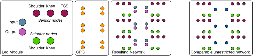
Figure 1: Hexaboard NMODE configuration vs. unrestricted configuration. FCS refers to foot contact sensors.

Next, we will discuss the six different types of nodes, which are; sensor, actuator, hidden, input, output, and connector. The first three node types are well-known from other neural network contexts. Sensor nodes receive input from the agent’s sensors and are typically equipped with a linear (id) transfer function. Analogously, actuator nodes are directly connected to the actuators of the agent, and finally, hidden nodes are only connected to other nodes within the same module. Actuator and hidden neurons are usually equipped with one of the two sigmoidal functions presented above. Two of the new node types are named input and output. The role of these nodes is to function as connectors between modules. Input nodes only allow connections from itself to other neurons within the module it is assigned to, whereas output nodes only allow connections from nodes of the corresponding module to itself. To connect a module with another module that has input and output nodes, the connecting module has to use a connector node. The connector node will copy the position and properties of the node it is referring to. In particular, this means that if a connector nodes refers to an input node, it will automatically become an output node of the connecting module.

As an example, consider the hexapod used in the first experiment presented below (see Sec. 3.1). Its NMODE structure is shown in Figure 1. Sensor nodes are shown in red, actuator nodes in green, input nodes in cyan, output nodes in purple, and finally, connector nodes in orange. In the experiment discussed below, only one leg module and one CPG module are evolved. By definition, a leg module controls a leg, which means that requires needs sensor and actuator nodes to access the leg’s state and control its movement. For a simple locomotion movement, the CPG does not require any sensor or actuator nodes. Instead, the CPG only consists of connector nodes to interface with the evolved leg modules. Because all legs are morphologically identical in this example, only one leg module has to be evolved, which is the used several times for the final controller (see Fig. 1).

We demonstrate the parameter reduction that results from this modularisation based on the hexapod example and with the assumption that the insertion of hidden units is not allowed. This allows us to calculate the maximal number of edge for a modularised and non-modularised neural network (see Fig. 1), where the latter means that synapses can connect any two neurons. It must be noted, that sensor nodes can only have outgoing connections in the current implementation, i.e., they only function as proxy for the sensor values. Let $n_{s,a,i,o,h}$ be the number of sensor, actuator, input, output, and hidden nodes. For a fair comparison, we replace all pairs of input/output nodes by a single hidden node in the unrestricted configuration, which follows structure that was used in [17, 31]. Then the dimension of the weight matrices for the two configurations is given by Tab. 1.

NMODE configuration: Leg Module

$n_{s}\cdot(n_{o}+n_{a})+n_{i}\cdot(n_{i}+n_{a})+n_{o}\cdot(n_{i}+n_{a})+n_{a} \cdot(n_{o}+n_{a})=21$

NMODE configuration: CPG Module

$n_{i}\cdot n_{o}+n_{o}\cdot n_{i}=72$

NMODE configuration: Total = 93

Unrestricted configuration:

$n_{s}\cdot(n_{h}+n_{a})+n_{h}\cdot(n_{h}+n_{a})+n_{a}\cdot(n_{h}+n_{a})=540$

Table 1: Comparison of search space dimension for the Hexapod example.

For the example of a six-legged walking machine with 2DOF per leg, we see that the unrestricted configuration has up to 540 free parameters that the evolutionary algorithm has to take care of, compared to the modularised network structure, which only requires the evolution of maximally 93 parameters. In other words, the search space in the unrestricted case is about $5.8$ times larger compared to the modularised case. The next section discusses the selection, mutation, and reproduction operators on modules.

2.2 Selection

We decided to use the simplest form of selection, which is a rank based approach. After evaluation, the individuals are ranked based on their fitness value. The top $n\%$ (user defined) are then selected for reproduction. In the previously used ENS³ approach [10, 14], offspring were assigned to individuals with respect to a Poisson distribution based on the individual’s fitness values. Individuals without offspring after the reproduction process, were removed from the population. An additional parameter allowed to save the best $n$ individuals, which might have not been assigned an offspring despite having a high fitness value. The idea was that, because of its stochastic nature, this selection method would provide more diversity in the population. We believe that the speciation method introduced by [23] is more valuable in this respect, which is why it will be included and evaluated in future versions of NMODE. We also believe that cross-over is more useful with respect to ensuring diversity in the population, which is why a crossover mechanism based on the exchange of modules is included (see below). In future versions of NMODE, we will evaluate a NEAT-based cross-over technique to allow crossover between two modules instead of a full exchange.

2.3 Reproduction

The task of the reproduction operator is to assign the right amount of offspring to each individual that was selected after the evaluation. By right amount we mean that the number of offspring assigned to each individual should reflect the individual’s fitness values. For this purpose, all fitness values are normalised in the following way:

$$s_{i} =\left(\frac{f_{i}-\min_{i}\{f_{i}\}}{\max_{i}\{f_{i}\}-\min_{i}\{f_{i}\}}\right)^{\eta}, r_{i} =\frac{s_{i}}{\sum_{i}s_{i}},$$ (4)

where $i=1,2,\ldots,N$ is the index of the $i$-th individual, and $f_{i}$ is the corresponding fitness value, $\eta$ is the elitism parameter, and $r_{i}$ is the reproduction factor. A constant value for $s_{i}$ is used, if $\max\{f_{i}\}=\min\{f_{i}\}$. A high value of $\eta$ leads to a concentration of the offspring to the individuals with the highest fitness values. Analogously, a low value of $\eta$ results in an equal distribution of offspring among the selected individual. The resulting reproduction factors $r_{i}$ sum up to one, which means that the normalised $r_{i}$ can directly be used to distribute the number of offspring.

One reason for the modularisation of the neural networks and the definition of the interface nodes is that the modules can easily be exchanged between individuals. If the cross-over parameter is positive, i.e. $\zeta>0$, then for each offspring (which is a copy of its mother) a father is chosen randomly from the set of parents depending on their normalised reproduction factor $r_{i}$. This means that individuals with a high reproduction will be chosen more often as a mating partners. If two mates are found, then $\zeta$ also determines the probability with which a module is chosen from the father instead of the mother. This can be fatal in many cases, because the modules were not co-evolved, and hence, there is a high probability that e.g. a leg module that works fine with a particular CPG will not work at all with another CPG. This is accounted for, because very fit individuals will often mate with themselves (due to their high fitness value), and hence, good networks will be preserved. On the other hand, less successful networks will more likely be crossed with more successful networks, which could increase their survival chances. As briefly mentioned above, one might think about using NEAT as a method to evolve networks within in module. This would then allow to cross module-networks instead of completely switching them. We will investigate this possibility in future versions of NMODE.

2.4 Mutation

NMODE is designed particularly to evolve neural networks of arbitrary structure while restricting the search space in an meaningful way. This means that the mutations are performed on the level of modules and not on the entire neural network. Consequently, in the following sections, $\mathcal{E}$ and $\mathcal{N}$ denote the set of all edges and nodes within a single module.

Synapse insertion

Because nodes have a three-dimensional position (see above), it makes sense to insert edges based on the Euclidean distance between nodes. Nodes which are closer together, will have a higher probability of being connected than those which are separated by a longer distance. This way, sensors and actuators which e.g. read and control the same joint are more likely to be connected early during the evolutionary process than sensors and actuators which have a larger distance. We will investigate how a distance-based edge generation method differs from an uniformly distributed insertion of edges with respect to the evolutionary success and the generated behaviours in an experiment discussed below (see Sec. 3.1). Both methods are explained in the following paragraph.

At first, NMODE generates a dis-connectivity matrix. This means, that the matrix $D$ has a positive, non-zero entry at $d_{ij}$ when the synapse from node $j$ to node $i$ does not exist. There are currently two ways in which the non-zero entries are calculated (see Alg. 1). The first possibility is to set them uniformly to one. This means that each new connection has the same probability of being created. This refers to a uniformly distributed insertion of synapses. The second possibility is to set the values proportionally to the distance between the two corresponding neurons. This means that neurons which are closer to each other will have a higher chance of being connected by a synapse. In both cases, each entry in the dis-connectivity matrix is then multiplied with the user-defined synapse insertion probability, which means that the resulting matrix determines with which probability each non-existing synapse will be created (see Alg. 1).

1:$p\in[0,1]$ $\triangleright$ Probability to insert a synapse

2:$u()\in[0,1]$ $\triangleright$ Function to draw a uniformly distributed random number

3:$D=(d_{ij})=0,\forall i,j=1,2,\ldots,N$

4:$\mathcal{E}\in\mathbb{N}^{2}$ $\triangleright$ is the set of all existing nodes, which is empty only for the initial generation.

5:for $i=1,2,\ldots,N$ do

6:     for $j=1,2,\ldots,N$ do

7:         if $(i,j)\not\in\mathcal{E}$ then

8:              if uniform then

9:                  $d_{ij}=1$

10:              else if distance then

11:                  $d_{ij}=\nicefrac{{1}}{{\mathrm{dist}(n_{i},n_{j})}}$

12:              end if

13:         end if

14:     end for

15:end for

16:$D=\frac{D}{\max D}$ $\triangleright$ Normalise $D$ such that the largest entry is equal to one.

17:for $i=1,2,\ldots,N$ do

18:     for $j=1,2,\ldots,N$ do

19:         if $u()<p\cdot d_{ij}$ then

20:              Add synapse $(i,j)$ to $\mathcal{E}$

21:         end if$u()<p_{si}$

22:     end for

23:end for

Algorithm 1 Synapse insertion

Synapse deletion

The user specifies how many synapses can be removed during the mutation of a module. Hence, if the user specifies $p=1$, than any fraction from $0\%$ to $100\%$ of the synapses can be deleted, whereas $p=0.5$ means that maximally $50\%$ of all existing synapses can be deleted. The synapse deletion algorithm is comparably simple (see Alg. 2).

1:$p\in[0,1]$ $\triangleright$ Probability to delete a synapse

2:$u()\in[0,1]$ $\triangleright$ Function to draw a uniformly distributed random number

3:$N=u()\cdot p\cdot|\mathcal{E}|$

4:for $i=1,2,\ldots,N$ do

5:     Delete a synapse randomly drawn from $\mathcal{E}$

6:end for

Algorithm 2 Synapse deletion

One could argue that this form of synapse insertion and deletion are too invasive, as they can both lead to significant changes of the network structure. This is intentional for the following reason. NMODE was not designed to be a biologically plausible evolutionary algorithm to understand how biology has evolved complex systems. NMODE was initiated to find controller for complex systems in cases where other approaches fail. In other words, the solution is more important than the algorithm that found it. Therefore, if a local maximum is reached, it is desirable to increase the stochastic search area to find other maxima. A good way of doing this is to significantly alter the structure of the neural network, which is why we allow such large structural variations.

Synapse modification

The modification of synapses is straight forward. Each synapse is modified with a probability specified by the experimenter. The parameter $\delta$ determines the maximal variation of the synapse and the max parameter determines the limit of the synaptic strength (see Alg. 3).

1:$p\in[0,1]$ $\triangleright$ Probability to modify a synapse

2:$m\in\mathbb{R}^{+}$ $\triangleright$ Maximal absolute value for the synaptic strength

3:$\delta\in\mathbb{R}^{+}$ $\triangleright$ Maximal absolute change of a synaptic strength

4:$u()\in[0,1]$ $\triangleright$ Function to draw a uniformly distributed random number

5:for $(i,u)\in\mathcal{E}$ do

6:     if $u()<p$ then

7:         $w_{ij}=w_{ij}+\delta(2u()-1)$

8:         Prune $w_{ij}$, such that $w_{ij}\in[-m,m]$.

9:     end if

10:end for

Algorithm 3 Synapse modification

Neuron insertion

In growing a network, it is useful to insert neurons carefully, without massive structural changes [27]. In our previous implementation [14, 10], we used to add a neuron and automatically connect it to a given percentage of the neural network. This means that every new neuron has a potentially large impact on the network structure, and hence, its function. We decided to insert neurons more carefully. Hence, we adopted NEAT’s method of inserting a neuron, which means that with probability $p$ a synapse is chosen which is split by the new neuron. The synaptic weight of the new incoming synapse is set to one, whereas the outgoing synaptic strength is equal to the strength of the original synapse (see Alg. 4). The new neurons position is set to centre of the original synapse.

1:$p\in[0,1]$ $\triangleright$ Probability to add a neuron

2:$u()\in[0,1]$ $\triangleright$ Function to draw a uniformly distributed random number

3:if $u()<p$ then

4:     $(i,j)$ is drawn uniformly from $\mathcal{E}$

5:     Insert new neuron $k$ in $\mathcal{N}$

6:     Remove $(i,j)$ from $\mathcal{E}$

7:     Add $(i,k)$ with $w_{ik}=1$ to $\mathcal{E}$

8:     Add $(k,j)$ with $w_{ki}=w_{ij}$ to $\mathcal{E}$

9:end if

Algorithm 4 Neuron insertion

Neuron deletion

Depending on the number of connections, the deletion of a neuron can have a strong influence on the function of the recurrent neural network. For this reason, neurons should be removed with care, which is why in each mutation at most one neuron is removed (see Alg. 5).

1:$p\in[0,1]$ $\triangleright$ Probability to remove a neuron

2:$u()\in[0,1]$ $\triangleright$ Function to draw a uniformly distributed random number

3:if $u()<p$ then

4:     Remove a neuron randomly drawn from $\mathcal{N}$

5:end if

Algorithm 5 neuron deletion

Neuron modification

Neurons are modified in the same way that synapses are modified. Each neuron is modified with the specified probability. The bias value is changed with the limits specified by $\delta$ and cropped within the limits of the specified maximal value (see Alg. 6)

1:$p\in[0,1]$ $\triangleright$ Probability to modify a neuron

2:$m\in\mathbb{R}^{+}$ $\triangleright$ Maximal absolute value for the bias

3:$\delta\in\mathbb{R}^{+}$ $\triangleright$ Maximal absolute change of the bias

4:$u()\in[0,1]$ $\triangleright$ Function to draw a uniformly distributed random number

5:for $n\in\mathcal{N}$ do

6:     if $u()<p$ then

7:         $b_{n}=b_{n}+\delta(2u()-1)$

8:         Prune $b_{n}$, such that $b_{n}\in[-m,m]$.

9:     end if

10:end for

Algorithm 6 neuron modification

2.5 Evaluation

NMODE is primarily designed to work with YARS, although other simulators and evaluation methods can be easily included too. YARS is a fast mobile robot simulator especially designed for evolutionary robotics. It uses the bullet physics engine [6] for the physics and Ogre3D [28] for the visualisation. Robots can be created in blender [2] and imported to YARS and blender animation data can be exported from YARS allowing to replay and render the simulation from any camera angle. YARS and NMODE are both available from GitHub [13, 12]. Therefore, the question of evaluation (except for a brief discussion on fitness functions below) will not be addressed in this work but in a following publication on the current version of YARS.

This section does not discuss fitness functions in general. There is a vast amount of literature available on this topic (see e.g. [15, 20])). Instead, this section describes how fitness functions are implemented in NMODE, because this is only part that requires programming by the user. Fitness functions are dynamically loaded during runtime of the NMODE executable. The name of the fitness function given in XML file must correspond to the name of the library. The class must inherit the Evaluate class and implement the following functions; void updateController(), void updateFitnessFunction(), bool abort(), void newIndividual(), void evaluationCompleted(). The first function updateController is called after each step in the simulation, e.g. after each update of the sensor states. All sensor values are presented in an one-dimensional array and can be used to calculate the intermediate fitness. The function abort is then checked by NMODE to see if the evaluation should be terminated early. This function can be used by the experimenter to indicate that some abort condition was met, e.g. if a collision with a wall occurred. If an individual reached the full evaluation time, the evaluationCompleted function will be called to allow post-processing. In the examples given below, the entropy [7] over joint angles could be used as part of the fitness function. This calculation only makes sense at the end of each evaluation for two reasons. First, the calculation of entropies can be very time consuming, and hence, should not be performed after every simulation update. Second, such calculations are most usefull if the full data is available, which is why the evaluationCompleted function was added. The newIndividual function is called at the beginning of each evaluation and is meant for the initialisation and resetting of variables.

This concludes the introduction of NMODE. The next section presents two experiments in which NMODE was used to evolve locomotion behaviours in YARS.

3 Experiments

In the following, we will present two different experiments, namely, Hexaboard and Svenja. The reason why we present these experiments is that the Hexaboard can be considered to be a standard hexapod morphology with 2DOF per leg (see Fig. 2). This is a kind of benchmark experiment to show how well NMODE performs on such tasks. The second experiment, Svenja, is a hexapod morphology that was freely modelled after an insect. It has four degrees of freedom in each leg and the three leg pairs are morphologically different (see Fig. 2). Svenja is particularly challenging to control because of the arrangements of the legs and actuators. Contrary to Hexaboard, one cannot use the same network for each leg, as the three leg pairs will have different tasks, due to their differing morphologies. The front legs will have to pull, while the rear legs will have to push. The two centre legs have the same morphology as Hexaboard’s legs, and hence, will have a similar task. Manually programming a behaviour for this morphology turned out to be very challenging. This experiment was also chosen to demonstrate that NMODE’s modularisation is well-suited for incremental evolution. Each leg-pair was evolved individually, with its own CPG. For the final evolutionary phase, the three disjunct networks were simply merged.

3.1 Hexaboard

This experiment was chosen because it is a good representation of a standard experiment in the context of embodied artificial intelligence. The task is to evolve a neural network for the locomotion of a six-legged walking machine. Most walking machines are constructed with identical legs, i.e. each leg has the same morphology and is attached to the main body in exactly the same way. This reduces the complexity of the control significantly, because the controller does not have to distinguish between different leg pairs. The movements of the two front legs have the same effect on the locomotion behaviour as the movements of the rear legs. This is in contrast to natural systems, e.g. cockroaches, for which the front legs perform a pulling movement, whereas the rear legs can be said to push. Later in this work, we will evolve a neural network for a hexapod with a more natural task distribution for its legs (see Sec. 3.2). In this section we will first concentrate on the standard configuration of six identical legs, which are mounted parallel to each other to a single segment (see Fig. 2).

For such a system, is it natural to assume that each leg should have the same local leg controller, because each leg should show the same behavioural pattern in e.g. a tripod walking gait. Hence, to reduce the search space, we only need to evolve a single leg controller and copy it five times for the final controller. In addition to the leg controller, only the connecting structure (central pattern generator or CPG) needs to be evolved, which means that the search space can be reduced significantly (see Tab. 1 an and Fig. 1). In what follows, we will first describe the morphology, followed by the user-defined evolution parameters, before the results are presented. It must be noted here, that all experiments were conducted as batch process, i.e., the parameters were set at the beginning of the experiments, kept constant and the same for all experiments. This is not how NMODE was intended to be used and other parameters might lead to even better results. The goal here is to show how fast NMODE can evolve a good behaviour for such a standard platform. The goal is not to evolve an optimal network structure (with respect to size and robustness against disturbances), which would require alternative growing and pruning phases, modification of fitness function parameters, etc., and hence, a monitoring of the evolutionary process. Interactive evolution would not allow to make statistical statements about the evolutionary progress, which is why we chose to evolve in batch mode.

3.1.1 Morphology

We chose Hexaboard as our experimental platform for two reasons. First, it is provided in the YARS distribution, which means that the results presented here can be easily verified, and second, it was successfully used in previous experiments [18]. Overall, the robot was designed especially for the purpose of learning locomotion, which means that the body part dimensions, weights, forces, angular range, etc. were set such that the system is highly dynamic but has a very low probability of flipping over. The exact parameters are presented in Table 1. Figure 2 visualises the arrangement of the joints and their rotation axes.

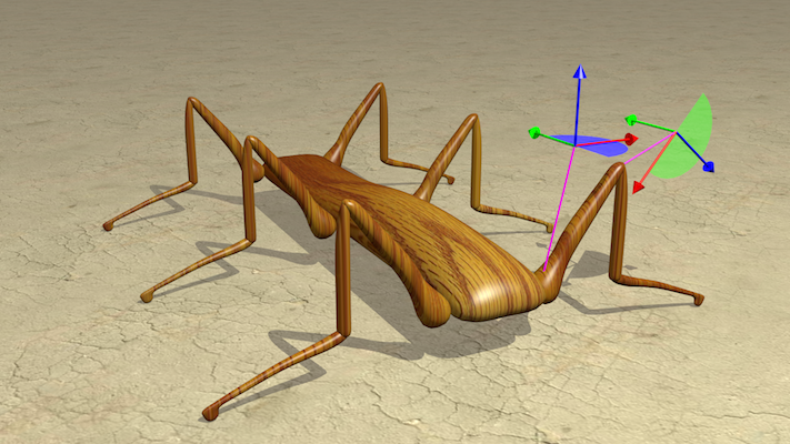
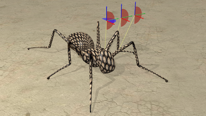
Figure 2: Experimental platforms. Left: Hexaboard is standard hexapod with 2DOF per leg. Right: Svenja is a hexapod that is loosely modelled after an insect with 4DOF per leg and two light sensors.

	Bounding Box (x,y,z)			Mass
Main Body	0.75 m	4.41 m	0.5 m	2.0 kg
Femur	0.23 m	0.23 m	1.17 m	0.2 kg
Tibia	0.1 m	0.09 m	0.9 m	0.15 kg
Tarsus	0.1 m	0.08 m	1.04 m	0.1 kg

	$\alpha_{\mathrm{min}}$	$\alpha_{\mathrm{max}}$	$F_{\mathrm{max}}$	$V_{\mathrm{max}}$
Shoulder	-35 ∘	35 ∘	20.0 $\nicefrac{{N}}{{m}}$	0.75 $\nicefrac{{rad}}{{s}}$
Knee	-15 ∘	25 ∘	20.0 $\nicefrac{{N}}{{m}}$	0.75 $\nicefrac{{rad}}{{s}}$

Table 2: Hexaboard’s specification

All shapes were modelled in blender and the visual appearance of the robot is equivalent to it’s physical form, which means that the shapes that are used for collision detection etc. are the same shapes that are also used for the visualisation. This is also true for Svenja (see below).

3.1.2 NMODE parameters

To evaluate how well NMODE evolves a locomotion network for a standard hexapod platform, we ran each experiment 10 times with the same set of parameters. From previous experience [17], we decided to focus primarily on the evolution of the connectivity structure and omitted the insertion and deletion of neurons in this set of experiments. Hence, the probability to add or remove a node was set to zero. For the reproduction parameters, we chose a population size of 100 with a selection pressure of 0.1. The elitism parameter is set to 10.0, which we determined empirically. Crossover was set to 0.1. The mutation parameters were set to node modification of 0.01 with a maximal absolute value for the bias of 1.0 and a maximal change of the bias value to 0.01. Edge modification was set to 0.2, with a maximum of 5.0 and a maximal step size of 0.5. Edges can be inserted with a probability of 0.05 and a maximal absolute synaptic strength of 1.0. For the experiment in which the probability of an edge insertion is dependent on the distance of the nodes, the minimal distance was set to 0.1, which means that neurons with a distance smaller than 10 cm are set to 10 cm (this also applies to self-connections).

3.1.3 Fitness Function

The fitness function is the summed distance in direction of the initial orientation of Hexaboard, which is along the positive $y$-axis. Let $t=1,2,\ldots,T$ indicate the time steps, then the fitness function is defined as

$$F =\sum_{t=1}^{T}y(t).$$ (5)

The reason for using the summed distance instead of the maximal distance is that a small progress in distance leads to higher selection pressure, i.e. significantly more offspring are assigned to individuals which are slightly better than their peers.

3.1.4 Results

The plot on the left-hand side of Figure 3 shows the fitness over generations for a uniform insertion of synapses, while the plot on the right-hand side of Figure 3 shows the fitness over generations for distance-based insertion of synapses. The standard deviations and mean values are taken with respect to all selected individuals of all 10 experimental trials. The smaller plots in each figure show the mean and standard deviation for only the best individuals over all 10 experiments. Hence, the large plots show the values for 100 individuals in each generation (10 for each of the 10 experiments), whereas the smaller plots only show the calculated values for 10 individuals (the best of each experiment). Figure 4 shows the resulting walking patterns for three different evolved individuals.

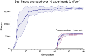
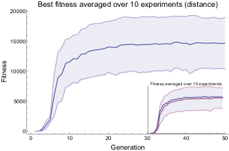
Figure 3: Hexaboard fitness. Left: Edges are added uniformly, which means that the distance between the connected node is not taken into account. Right: The probability of inserting and edge decreases with the distance between the connected nodes. Both plots show the best fitness averaged over 10 experiments, with the corresponding standard deviation. The picture-in-picture plots show the fitness of all selected individuals in each generation averaged over 10 experiments. For comparison, the best fitness values in each generation is added to the smaller plot as blue line.

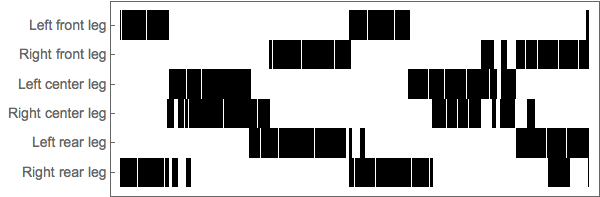
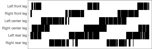
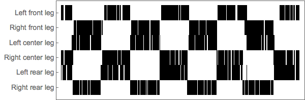
Figure 4: Examples of evolved walking patterns for Hexaboard. Left and centre: These are two walking patterns that resulted from inserting edges dependent on the distance. Right: The classical tripod walking behaviour that was most dominant when synapses were inserted uniformly. The tripod walking pattern was also found in experiments in which the distance-based approach was used, but there was a larger variety compared to the uniform approach. For the latter, the walking patterns mostly differed in the length of the leg stance and swing phases. Videos of the walking patterns are available online. In the same order as they are shown above: https://youtu.be/a0OtDBHpe1c, https://youtu.be/UwFKYTIn56w, https://youtu.be/fZlmPTSmCi0.

From the results shown in Figs. 3 and 4 we can draw the following conclusions. First, both approaches lead to a good locomotion behaviour already after approximately 10 generations. To the best of the authors knowledge, no similar results were published for any other evolutionary algorithm. The second conclusion is that both approaches, uniform and distance-based insertion of synapses on average lead to similar results. In both cases, the best walking behaviours showed a tripod walking behaviour (see Fig. 4, left-hand side). Note that the fitness function (see Eq. (5)) only favours fast walking but does not reward a specific walking pattern. In the case of the distance-based approach, we see a higher variance in the fitness over the different experiments. This is also reflected in the resulting walking patterns. Two examples of the best behaviours from the ten experiments with distance-based insertion of synapses are shown in Figure 4 (centre and right-hand side). This leads to the conclusion that if optimality is the highest priority, uniform insertion of synapses (position-independent) seems to be the approach of choice, whereas distance-based insertion of synapses should be used if diversity of the solutions is desired.

3.2 Svenja

Svenja was chosen for presentation here to demonstrate how NMODE can be used for incremental evolution of complex systems. Svenja’s morphology is significantly more complex compared to Hexaboard for four main reasons. First, each leg has 4 DOF (instead of 2). Second, the leg-pairs significantly differ in their shape and attachment to the main body. Third, the main body is segmented, with a non-even distribution of the weight, in particular, the rear end of Svenja is twice as heavy as the head, which means that the center of mass is not within the convex hull of the leg’s anchor points (see Fig. 2 and Tab. 3). Fourth, due to the leg morphology and weight distribution, Svenja is very likely to flip over if the legs are not moved properly. To further increase the difficulty of the task, we included obstacles in the environment (see Fig. 5, right-hand side).

The approach we chose to evolve Svenja is incremental in the sense that we first evolve every leg-pair independently and then merge the resulting networks to evolve the coordination among the legs. As for Hexaboard, evolution was performed as a batch process, with initially fixed parameters.

Figure 5 sketches the incremental approach. On the left-hand side, the evolution of each leg pair is shown. The leg-pairs were evolved with a single leg controller, that was mirrored for the other leg, and a CPG that only consisted of connector nodes to the leg modules (one input and one output node per leg module). For the final controller (see Fig. 5, left-hand side), the three leg modules were simply appended in a single XML file. The three disjunct CPGs were appended into a single module, which was then appended to the list of leg modules. A small Python script was enough to automate this process, which also could have been done manually with a simple XML editor. Figure 5 (right-hand side), shows the three different evolutionary settings for the first step of the incremental evolution. The main body is attached to an invisible rail that only allows movements along the $z$- and $y$-axes (up/down and forwards/backwards movements). Movements along the $x$-axes and rotations in general are constrained to zero.

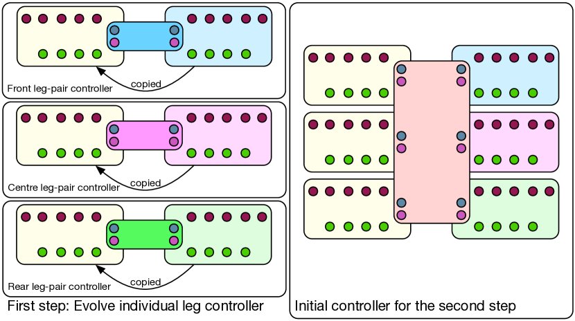
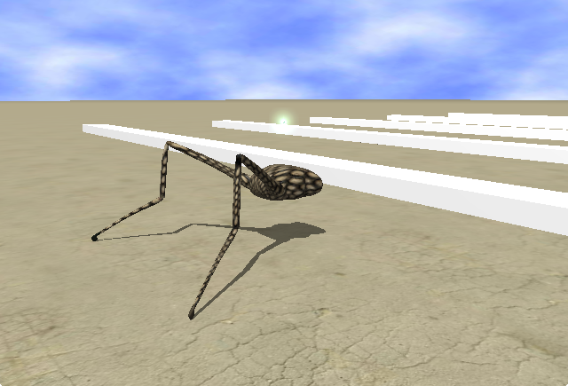
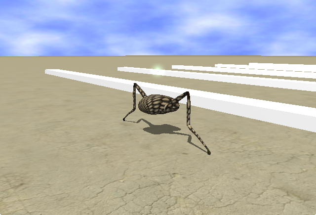
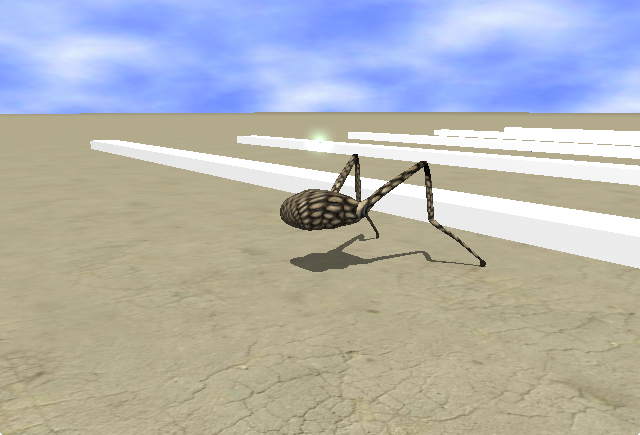
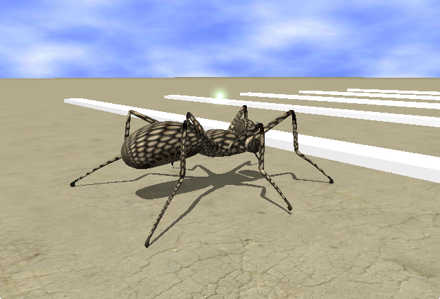
Figure 5: Incremental evolution of Svenja. Left-hand side: Controller set-up. First, for each leg-pair, individual controller are evolved (first image on the left hand side). The evolved leg controller are then combined to control the full morphology (second image on the left-hand side). Note that the combination of the three controller is straight forward (see text for details). Right-hand side: The corresponding evaluation environments in YARS. From left to right and top to bottom, rear legs, centre legs, front legs, and full morphology.

In the following paragraphs, we will first give the specifications of the morphology, then describe the NMODE parameters and fitness function, before the results are presented.

3.2.1 Morphology

Svenja has 4DOF of which the first are located in the first joint. This means that the femur can be rotated around two axes simultaneously (see Fig. 2). The other two DOFs allow rotations around a single axes and connect the femur with the tibia and the tibia with the tarsus. Svenja’s main body consists of three segments. This affects the centre of mass of the entire system. The head and main segments (two which all legs are attached) have a weight of 10 kg, whereas the rear segment has a weight of 20 kg. The full specifications of Svenja are summarised in Table 3 (see Appendix).

3.2.2 NMODE parameters

During the first phase, three independent evolutionary experiments were conducted, one for each leg pair. In all runs (repeated five times each), we used the same NMODE parameters, which are set to; life time is 500 iterations, generations are limited to 250, population size is set to 50, elite pressure is set to 5.0, with a cross over probability of 0.25, node mutation probability is set to 0.1, with a maximum of 1.0 and maximal step width of 0.2, nodes are added with with a probability of 0.1 (and a maximal bias values of 1.0) and deleted with with probability of 0.1, edge mutation probability is set to 0.3, with a maximum of 5.0 and maximal step width of 1.0, edges are added with with a probability of 0.05 (and a synaptic strength of 1.0) and deleted with with probability of 0.05.

3.2.3 Fitness function

The main part of the fitness is equivalent to the fitness function used for Hexaboard, which means that we used the sum over the main body’s $y$-coordinate in the world coordinate frame. For the evolution of the leg pairs, an additional punishment was added for changes of the main body’s $z$-coordinate. This means that in principle each evolved leg pair run could result in different walking heights as long as the main body height changes were minimal. The fitness function read as:

$$F=\sum_{t=1}^{t}[y(t)-\gamma(z(t)-z(t-1))],$$ (6)

where $z(0)$ is the initial position of the main body before the simulation is iterated for the first time.

3.2.4 Results

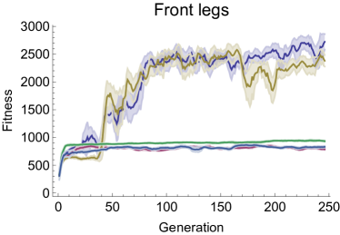
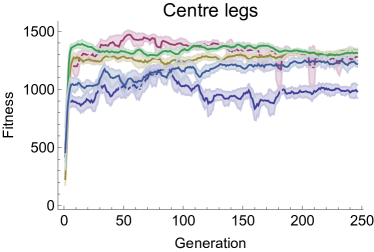
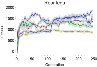
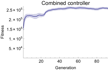
Figure 6: Fitness of Svenja controller over generations. For the final controller (lower right-hand side), the best individuals for the five runs of each leg pair were chosen. For details, please read the main text.

The results are captured in Figure 6 and Figure 7. Figure 6 shows the fitness over generations for the leg pairs (five runs each) and the evolution of the merged leg-pair controller. Figure 7 shows the final behaviour for a sequence in which Svenja climbs over an obstacle. Videos of all evolved behaviours can also be found online.

The first observation is that the front legs seem to be more difficult to evolve than the other two leg pairs. It took about 100 generations to evolve a good behaviour compared to approximately 10-20 generations for the centre and rear leg pairs. The reason is that the way the front legs are attached to the main body makes it more difficult for them to climb over the obstacles (see Fig. 5, right-hand side). In early generations, each leg-pair’s controller would start with oscillatory movements of low amplitude and high frequency. For the rear and centre leg-pairs small increases of the amplitude would already increase the likelihood of climbing the obstacle, while the front legs would still be blocked by the first obstacle. The reason is that the oscillatory leg movements of the first leg pair repel the main body more easily from the obstacle than it is the case for the other leg pairs.

Another observation is that the combined controller very quickly learned to coordinate the leg pairs. Remember that each leg pair was evolved independently, with no restriction of the walking height or walking pattern. Yet, within less than 10 generations the first coordination occurs. After approximately 20 generations a good walking behaviour has been found which is shown in Figure 7.

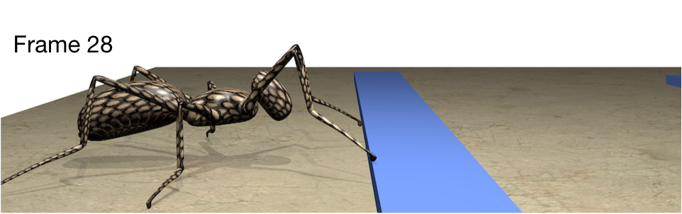
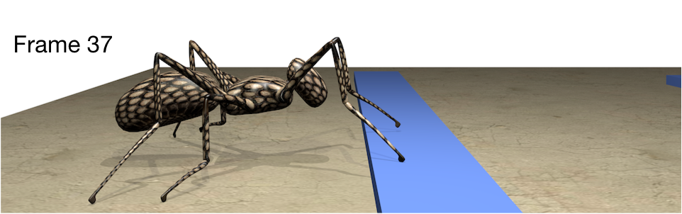
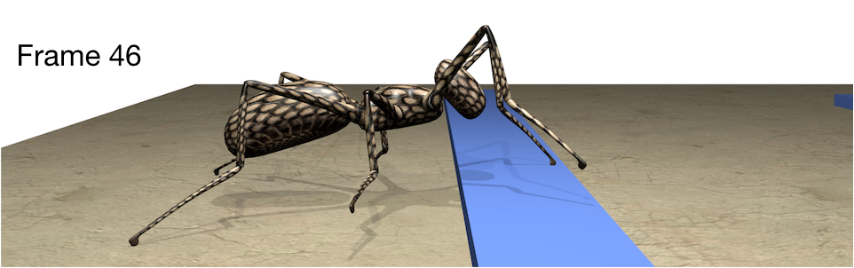
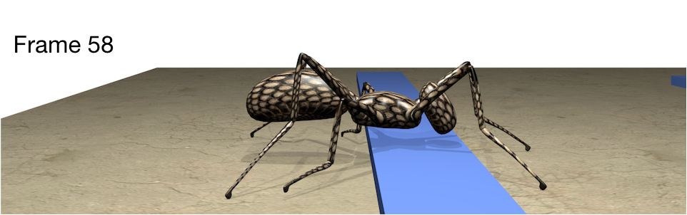
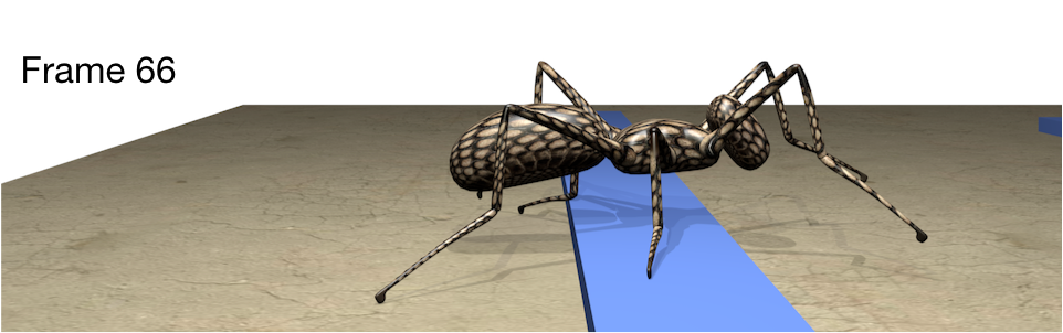
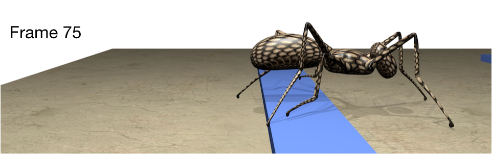
Figure 7: This figure shows the walking behaviour of Svenja. Frames 28, 37, 46, 58, 66, and 75 are shown here (rendered with blender), which is equivalent to approximately 2.5 s.

In total, the evolution of a good walking behaviour for Svenja required only a few of hours of CPU time. It must be noted again, that this process was done as a batch process, and hence, the final behaviour is not optimal with respect to size, robustness, etc. Still, this experiment shows that a behaviour for a complex morphology such as Svenja can be learned very fast with NMODE.

4 Discussion

We presented a novel approach to artificial evolution of neural networks and demonstrated its applicability in two experiments. NMODE was not developed isolated from current research in evolutionary robotics, rather ideas of different approaches were combined in a minimalistic way. NMODE builds upon the main authors own experience in evolutionary robotics (ISEE), experience with a collaborator’s software framework (NERD) and own experience and literature research on the currently most dominant approach (HyperNEAT). We showed that NMODE is able to evolve a locomotion behaviour for two different hexapod experiments in very few generations. To the best of the authors knowledge, no similar results have been published so far, which shows the usefulness of NMODE in generating interesting behaviours for complex morphologies.

This said, the development of NMODE is not completed yet. On the short-term, we will evaluate NEAT as a method to evolve the networks within a module to allow crossover between modules instead of completely switching modules. In addition, we will also include NEAT’s speciation method to protect innovations. Most importantly, We will have to show that NMODE is able to evolve non-reactive behaviours for complex morphologies, which is the topic of ongoing experiments.

5 Acknowledgement

This work was partly funded by the DFG-SPP 1527 ,,Autonomous Learning”

Appendix A Svenja specification

	Bounding Box (x,y,z)			Mass
Head	0.614 m	0.614 m	0.812 m	10.0 kg
Main Body	0.976 m	1.107 m	0.552 m	10.0 kg
Rear	0.832 m	1.643 m	0.860 m	20.0 kg
Front femur	0.612 m	0.945 m	0.977 m	2.0 kg
Front tibia	0.204 m	0.297 m	0.901 m	1.5 kg
Front tarsus	0.611 m	1.026 m	0.444 m	1.0 kg
Centre femur	0.767 m	0.230 m	1.972 m	2.0 kg
Centre tibia	0.103 m	0.094 m	0.909 m	1.5 kg
Centre tarsus	0.973 m	0.083 m	0.436 m	1.0 kg
Rear femur	0.804 m	1.283 m	1.004 m	2.0 kg
Rear tibia	0.273 m	0.417 m	0.897 m	1.5 kg
Rear tarsus	0.729 m	1.230 m	0.446 m	1.0 kg

	$\alpha_{\mathrm{min}}$	$\alpha_{\mathrm{max}}$	$F_{\mathrm{max}}$	$V_{\mathrm{max}}$
Front Ma-Fe 1	-5 ∘	20 ∘	7.5 $\nicefrac{{N}}{{m}}$	0.5 $\nicefrac{{rad}}{{s}}$
Front Ma-Fe 2	-25 ∘	35 ∘	7.5 $\nicefrac{{N}}{{m}}$	0.5 $\nicefrac{{rad}}{{s}}$
Front Fe-Ti	-10 ∘	10 ∘	7.5 $\nicefrac{{N}}{{m}}$	0.5 $\nicefrac{{rad}}{{s}}$
Front Ti-Ta	-30 ∘	5 ∘	7.5 $\nicefrac{{N}}{{m}}$	0.5 $\nicefrac{{rad}}{{s}}$
Centre Ma-Fe 1	-0.5 ∘	45 ∘	7.5 $\nicefrac{{N}}{{m}}$	0.5 $\nicefrac{{rad}}{{s}}$
Centre Ma-Fe 2	-45 ∘	45 ∘	7.5 $\nicefrac{{N}}{{m}}$	0.5 $\nicefrac{{rad}}{{s}}$
Centre Fe-Ti	-30 ∘	5 ∘	7.5 $\nicefrac{{N}}{{m}}$	0.5 $\nicefrac{{rad}}{{s}}$
Centre Ti-Ta	-2.5 ∘	45 ∘	7.5 $\nicefrac{{N}}{{m}}$	0.5 $\nicefrac{{rad}}{{s}}$
Rear Ma-Fe 1	-5 ∘	20 ∘	7.5 $\nicefrac{{N}}{{m}}$	0.5 $\nicefrac{{rad}}{{s}}$
Rear Ma-Fe 2	-30 ∘	20 ∘	7.5 $\nicefrac{{N}}{{m}}$	0.5 $\nicefrac{{rad}}{{s}}$
Rear Fe-Ti	-5 ∘	27.5 ∘	7.5 $\nicefrac{{N}}{{m}}$	0.5 $\nicefrac{{rad}}{{s}}$
Rear Ti-Ta	-25 ∘	20 ∘	7.5 $\nicefrac{{N}}{{m}}$	0.5 $\nicefrac{{rad}}{{s}}$

Table 3: Svenja’s specification. Please note, that the domains for the angular position are given for the legs on the right side. Depending on how the joint is attached, the values have different meaning, i.e., in which direction the leg will move give an specific value. The numbers are presented here to given an impression of the leg’s moving ranges.

References

- [1] Auerbach, J.E., Bongard, J.C.: Environmental influence on the evolution of morphological complexity in machines. PLoS Comput Biol 10(1), 1–17 (2014)
- [2] Blender Foundatation: blender 2.78a. \urlwww.blender.org (2017)
- [3] Braitenberg, V.: Vehicles. MIT Press, Cambridge MA (1984)
- [4] Clune, J., Beckmann, B.E., Ofria, C., Pennock, R.T.: Evolving coordinated quadruped gaits with the hyperneat generative encoding. In: Proceedings of the Eleventh Conference on Congress on Evolutionary Computation, CEC’09, pp. 2764–2771. IEEE Press, Piscataway, NJ, USA (2009)
- [5] Clune, J., Lipson, H.: Evolving 3d objects with a generative encoding inspired by developmental biology. SIGEVOlution 5(4), 2–12 (2011)
- [6] Coumans, E.: Bullet physics simulation. In: ACM SIGGRAPH 2015 Courses, SIGGRAPH ’15. ACM, New York, NY, USA (2015)
- [7] Cover, T.M., Thomas, J.A.: Elements of Information Theory, vol. 2nd. Wiley, Hoboken, New Jersey, USA (2006)
- [8] Cruse, H.: What mechanisms coordinate leg movement in walking arthropods? Trends in Neurosciences 13(1), 15 – 21 (1990)
- [9] Cruse, H., Kindermann, T., Schumm, M., Dean, J., Schmitz, J.: Walknet—a biologically inspired network to control six-legged walking. Neural Networks 11(7–8), 1435 – 1447 (1998)
- [10] Dieckmann, U., Pasemann, F.: Coevolution as an autonomous learning strategy for neuromodules. In: Proceedings of the European Conference on Artificial Life (ECAL’95). Granada, Spain (1995)
- [11] Ekeberg, Ö., Blümel, M., Büschges, A.: Dynamic simulation of insect walking. Arthropod Structure & Development 33(3), 287 – 300 (2004)
- [12] Ghazi-Zahedi, K.: NMODE Github Repository. \urlhttps://github.com/kzahedi/NMODE (2016)
- [13] Ghazi-Zahedi, K.: YARS Github Repository. \urlhttps://github.com/kzahedi/YARS (2016)
- [14] Ghazi-Zahedi, K.M.: Self-regulating neurons. a model for synaptic plasticity in artificial recurrent neural networks. Ph.D. thesis, Univeristy of Osnabrück (2009)
- [15] Holland, J.H.: Adaptation in Natural and Artificial Systems: An Introductory Analysis with Applications to Biology, Control and Artificial Intelligence. MIT Press, Cambridge, MA, USA (1992)
- [16] Ijspeert, A.J.: Central pattern generators for locomotion control in animals and robots: A review. Neural Networks 21(4), 642 – 653 (2008)
- [17] Markelić, I., Zahedi, K.: An evolved neural network for fast quadrupedal locomotion. In: M. Xie, S. Dubowsky (eds.) Advances in Climbing and Walking Robots, Proceedings of 10th International Conference (CLAWAR 2007), pp. 65–72. World Scientific Publishing Company (2007)
- [18] Montúfar, G., Ghazi-Zahedi, K., Ay, N.: A theory of cheap control in embodied systems. PLoS Comput Biol 11(9), e1004,427 (2015)
- [19] Nicholas Cheney, J.C., Lipson, H.: Evolved electrophysiological soft robots. In: Proceedings of the Fourteenth International Conference on the Synthesis and Simulation of Living Systems (ALIFE 14) (2014)
- [20] Nolfi, S., Floreano, D.: Evolutionary Robotics. MIT Press (2000)
- [21] Open Robotics Foundation: (2016). URL \urlhttp://gazebosim.org
- [22] Rempis, C., Thomas, V., Bachmann, F., Pasemann, F.: NERD Neurodynamics and Evolutionary Robotics Development Kit, pp. 121–132. Springer Berlin Heidelberg, Berlin, Heidelberg (2010)
- [23] Risi, S., Stanley, K.O.: An enhanced hypercube-based encoding for evolving the placement, density, and connectivity of neurons. Artif Life 18(4), 331–63 (2012)
- [24] Secretan, J., Beato, N., D’Ambrosio, D.B., Rodriguez, A., Campbell, A., Folsom-Kovarik, J.T., Stanley, K.O.: Picbreeder: A case study in collaborative evolutionary exploration of design space. Evolutionary Computation 19(3), 373–403 (2011)
- [25] Sims, K.: Evolving 3d morphology and behavior by competition. Artificial Life 1(4), 353–372 (1994)
- [26] Sims, K.: Evolving virtual creatures. In: SIGGRAPH ’94: Proceedings of the 21st annual conference on Computer graphics and interactive techniques, pp. 15–22. ACM, New York, NY, USA (1994)
- [27] Stanley, K.O., Miikkulainen, R.: Evolving neural networks through augmenting topologies. Evol. Comput. 10(2), 99–127 (2002)
- [28] Streeting, S., Xie, J., Castaneda, P.J., Muldowney, T., Doyle, J., O’Sullivan, J., van der Laan, W.J.: Ogre. \urlhttp://www.ogre3d.org (2006)
- [29] Twickel, A., Büschges, A., Pasemann, F.: Deriving neural network controllers from neuro-biological data: implementation of a single-leg stick insect controller. Biological Cybernetics 104(1-2), 95–119 (2011)
- [30] von Twickel, A., Hild, M., Siedel, T., Patel, V., Pasemann, F.: Neural control of a modular multi-legged walking machine: Simulation and hardware. Robotics and Autonomous Systems 60(2), 227 – 241 (2012)
- [31] Zahedi, K., Martius, G., Ay, N.: Linear combination of one-step predictive information with an external reward in an episodic policy gradient setting: a critical analysis. Frontiers in Psychology 4(801) (2013)