Lozenge tiling dynamics and convergence to the hydrodynamic equation

Abstract.

We study a reversible continuous-time Markov dynamics of a discrete $(2+1)$-dimensional interface. This can be alternatively viewed as a dynamics of lozenge tilings of the $L\times L$ torus, or as a conservative dynamics for a two-dimensional system of interlaced particles. The particle interlacement constraints imply that the equilibrium measures are far from being product Bernoulli: particle correlations decay like the inverse distance squared and interface height fluctuations behave on large scales like a massless Gaussian field. We consider a particular choice of the transition rates, originally proposed in [15]: in terms of interlaced particles, a particle jump of length $n$ that preserves the interlacement constraints has rate $1/(2n)$. This dynamics presents special features: the average mutual volume between two interface configurations decreases with time [15] and a certain one-dimensional projection of the dynamics is described by the heat equation [21].

In this work we prove a hydrodynamic limit: after a diffusive rescaling of time and space, the height function evolution tends as $L\to\infty$ to the solution of a non-linear parabolic PDE. The initial profile is assumed to be $C^{2}$ differentiable and to contain no “frozen region”. The explicit form of the PDE was recently conjectured [13] on the basis of local equilibrium considerations. In contrast with the hydrodynamic equation for the Langevin dynamics of the Ginzburg-Landau model [7, 16], here the mobility coefficient turns out to be a non-trivial function of the interface slope.

2010 Mathematics Subject Classification: 60K35, 82C20, 52C20
Keywords: Lozenge tilings, Glauber dynamics, Hydrodynamic limit

1. Introduction

This work is motivated by the problem of understanding the large-scale limit of stochastic interface evolution [19, 6]. More precisely we are interested in the motion of the interface between two stable thermodynamic phases in a $(d+1)$-dimensional medium. Needless to say, the physically most interesting case is that of $d=2$. The motion results from thermal fluctuations; overall the interface tends to flatten, thereby minimizing its free energy.

Mathematically we consider an effective interface approximation where the internal structure of the two phases above and below the interface is disregarded and the $d$-dimensional interface is modeled as the graph of a function from $\mathbb{R}^{d}$ to $\mathbb{R}$ (or some discretized version of this). The physical rationale behind this approximation is a time-scale separation: the internal degrees of freedom of the two phases relax much faster than those of the interface. The effect of thermal fluctuations is modeled as a Markov chain and the fact that phases are in coexistence translates to reversibility of that chain.

On phenomenological grounds [19] one expects that, on sufficiently coarse scales, the interface dynamics is deterministic and described by a hydrodynamic equation of the type

$$\partial_{t}\psi(x,t)=-\mu(\nabla\psi(x,t))\frac{\delta F[\psi]}{\delta\psi(x,t)},$$ (1.1)

where $F[\psi]$ is the equilibrium surface free energy and $\mu(\nabla\psi)$ is a mobility coefficient, that depends on the details of the dynamics. Note that, without the prefactor $\mu$, (1.1) would be simply the gradient flow associated with the surface energy functional. We can therefore interpret $\mu$ as describing how effective the relaxation produced by the dynamics is, hence the name “mobility”. The relevant space-time rescaling where the behavior described by (1.1) should emerge is the diffusive one.

Writing $F$ as the integral of the slope-dependent surface tension,

$$F[\psi]=\int\mathrm{d}x_{1}\mathrm{d}x_{2}\,\sigma(\nabla\psi),$$ (1.2)

the equation takes the parabolic form

$$\partial_{t}\psi=\mu(\nabla\psi)\sum_{i,j=1,2}\sigma_{i,j}(\nabla\psi)\frac{\partial^{2}}{\partial_{x_{i}}\partial_{x_{j}}}\psi$$ (1.3)

where parabolicity derives from convexity of $\sigma$. In general, the PDE (1.3) is non-linear and the mobility is expected to be a non-trivial function of the slope.

It is very difficult, in particular if $d>1$, to prove convergence to a hydrodynamic equation starting from a non-trivial microscopic model. Even worse, in general it is not possible to guess, even heuristically, an explicit expression for the mobility; in fact, its expression as provided by the Green-Kubo formula involves an integral of space-time correlations computed in the stationary states [19]. Exceptions where $\mu$ can be written down explicitly are usually models where the dynamics satisfies some form of “gradient condition”, i.e. the microscopic current is the lattice gradient of some function [18]. The only example we know of a rigorous proof of the hydrodynamic limit for a $d>1$ diffusive interface dynamics is the work [7] by Funaki and Spohn. There, the Langevin dynamics for the $d\geq 1$ Ginzburg-Landau model with symmetric and convex potential is studied and the convergence to a hydrodynamic limit of the type (1.3) is proven. See also [16] where the analogous result is proven in a domain with Dirichlet instead of periodic boundary conditions. It is important to remark that for the Ginzburg-Landau model the mobility turns out to be a constant, that can be set to $1$ by a trivial time-change.

In dimension $d=1$, instead, natural Markov dynamics of discrete interfaces are provided by conservative lattice gases on $\mathbb{Z}$ (e.g. symmetric exclusion processes or zero-range processes), just by interpreting the number of particles at site $x$ as the interface gradient $\phi(x)-\phi(x-1)$ at $x$. Similarly, conservative continuous spin models on $\mathbb{Z}$ translate into Markov dynamics for one-dimensional interface models with continuous heights. Then, a hydrodynamic limit for the height function $\phi$ follows from that for the particle density (see e.g. [11, Ch. 4 and 5] for the symmetric simple exclusion and for a class of zero-range processes, and for instance [5] for the $d=1$ Ginzburg-Landau model). For $d>1$, instead, there is in general no natural way of associating a height function to a particle system on $\mathbb{Z}^{d}$.

In the present work, we study a two-dimensional stochastic interface evolution for which we can obtain a hydrodynamic limit of the type (1.3). Our model is very different from the Ginzburg-Landau one. First of all, the interface is discrete (heights take integer values) so that the dynamics is a Markov jump process rather than a diffusion. More importantly, the mobility coefficient $\mu$ in the limit PDE is a non-constant (and actually non-linear) function of the interface slope.

The state space of our Markov chain is the set of lozenge tilings of the two-dimensional triangular lattice, or more precisely of its $L\times L$ periodization. Lozenge tilings of the triangular lattice are well known to be in bijection with perfect matchings (aka dimer coverings) of the dual lattice, which is the honeycomb lattice $\mathcal{H}$. See Fig. 1.

Figure 1. The bijection between dimer coverings of $\mathcal{H}$ (left) and lozenge tilings of the triangular lattice (right). The horizontal dimers will be called “particles”.

On the other hand, since $\mathcal{H}$ is planar and bipartite, its perfect matchings are in bijection with a height function defined on its faces, see Fig. 2. This height function will then be our model of the discrete two-dimensional interface.

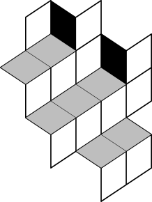
Figure 2. The lozenge tiling of Fig. 1, seen as a stepped two-dimensional surface representing the boundary of a pile of unit three-dimensional cubes.

The dynamics we study is reversible with respect to a two-parameter family of ergodic Gibbs measures, that are locally uniform measures on lozenge tilings. These measures are labelled by the two parameters of the interface slope and have a determinantal representation [10]. It is important to recall that such measures are far from looking like product Bernoulli measures: indeed, correlations decay like the inverse distance squared, while the height function itself tends in the large-scale limit to a two-dimensional massless Gaussian field [10, 9].

Starting with Section 2 we will adopt the dimer instead of the tiling point of view, and actually we will view the dimer configuration as an interacting particle system (“particles” being the horizontal dimers as in Figure 1). Such particles satisfy particular interlacement conditions, recalled in Section 2.

The updates of the dynamics consist in a horizontal dimer (or particle) jumping a certain distance $n$ vertically (up or down) in the hexagonal lattice, and such a transition will be assigned a rate $1/(2n)$ (the prefactor $1/2$ is there just to conform with the previous literature). See Section 2 for a precise definition. The jumps are not always allowed, not only because particles cannot superpose, but also because jumps cannot violate the above-mentioned interlacement constraints. This point is very important: in fact, it is the interlacement constraints that are responsible for the long-range correlations in the equilibrium measure. If instead we had only the exclusion constraint, the equilibrium measure would be Bernoulli.

Let us call “long-jump dynamics” the lozenge tiling dynamics just described, to distinguish it from the “single-flip Glauber dynamics” where only jumps of length $|n|=1$ are allowed. Let us mention that the single-flip dynamics is equivalent to the Glauber dynamics of the three-dimensional Ising model at zero temperature with Dobrushin boundary conditions [1]. The long-jump dynamics has an interesting story. It was originally introduced in [15] with the goal of providing a Markov chain that approaches the uniform measure on tilings, in variation distance, in a time that is polynomial in the system size $L$. In fact, the key point is that the mutual volume between two interface configurations is a super-martingale which, together with attractiveness of the dynamics, allows one to deduce polynomial mixing via coupling arguments. Later, in [21] it was proven that the total variation mixing time of the long-jump dynamics is actually of order $L^{2}\log L$, and that (in special domains) a particular one-dimensional projection of the height function evolves according to the one-dimensional heat equation. The results of [15, 21] were used as a building block in [1, 12] to prove that, under some conditions on the geometry of the domain, the mixing time of the single-flip Glauber dynamics is of order $L^{2+o(1)}$, like that of the long-jump dynamics. Finally, in [13] we discovered that, in contrast with the single-flip dynamics, the long-jump one satisfies certain identities, that allow to conjecture an explicit form for the hydrodynamic equation, cf. (2.10) or equivalently (2.12). While the dynamics does not satisfy a gradient condition in the usual sense that the microscopic current is a discrete gradient, still a discrete summation by parts causes the “dangerous” part in the mobility coefficient, the one involving space-time correlations, to vanish [13, Sec. 4]. A reflection of this fact is the summation by parts that takes place in Proposition 4.3 below.

In the present work, we prove rigorously the convergence to the hydrodynamic equation, in the case of periodic boundary conditions, under suitable smoothness assumptions on the initial profile. See Theorem 2.7.

The strong correlations in the invariant measures seem to prevent an approach to the hydrodynamic limit problem based on the application of classical methods going through one- and two-block estimates [18, 11]. Instead, broadly speaking, the proof of our result follows a scheme that is similar to that of [7] for the Ginzburg-Landau model, that builds on an extension of the so-called $H^{-1}$ (norm) method first introduced by Chang and Yau [2]. The basic idea of the method is to prove that the time-derivative of the ${\mathbb{L}}^{2}$ distance between the solution of the PDE and the randomly evolving interface is non-positive in the infinite volume limit. There are however important differences between the application of the method to the Ginzburg-Landau model and to ours, and here we mention two of them (see also Remark 5.5). First of all, one of the key points in [7] is an a-priori ${\mathbb{L}}^{2}$ control of interface gradients out of equilibrium, see Lemma 4.1 there, which is based on a simple coupling argument, that works because the interaction potential is assumed to be strictly convex. In our case the analog would be an a-priori control of the variable we call $k$ in (4.2), that determines how far particles can jump. The coupling argument however does not work, probably because the interaction in our model is not strictly convex, as witnessed by the fact that the position of a particle given its neighbors is uniformly distributed in the equilibrium state. Therefore, we have to proceed differently to get tightness of $k$, see e.g. Proposition 4.8. Secondly, the fact that the mobility is constant for the Ginzburg-Landau model played an important role in [7] and was behind the fact that the time derivative of the $\mathbb{L}^{2}$ distance between the randomly evolving interface and the solution of the deterministic hydrodynamic equation is negative. In fact, the negativity of this derivative is basically a consequence of convexity of the surface tension, see [7, Eq. (5.7)] and subsequent discussion. Contraction of the $\mathbb{L}^{2}$ norm holds also for our model but it seems to be more subtle, as it requires the negativity of a certain function (cf. (6.17)), a fact that does not follow simply from a thermodynamic convexity.

Our result raises interesting questions that we leave for future research: notably, the study of space-time correlations of height fluctuations around the limit PDE and the proof of the convergence to the hydrodynamic limit when boundary conditions are not periodic, especially when boundary conditions are such as to impose frozen regions in the equilibrium macroscopic shape [9].

Organization of the article

In Section 2, we introduce more precisely our model and we state our main result, Theorem 2.7: the convergence of the height function to the solution of an explicit deterministic PDE. This equation is of parabolic, non-linear type and in Section 3 we deduce existence and regularity of its solution (i.e. statement (i) of Theorem 2.7) from known results on parabolic PDEs. Sections 4 to 6, that are the bulk of the work, contain the proof of item (ii) in Theorem 2.7, i.e. the hydrodynamic limit convergence statement itself. A short reader’s guide to the structure of the proof is given at the end of Section 2.

2. Model and results

2.1. Dimer configurations and height function

Let $\mathcal{H}$ denote the infinite planar honeycomb lattice and let $\hat{e}_{1},\hat{e}_{2},\hat{e}_{3}$ be the unit vectors depicted in Figure 3. The dual lattice $\mathcal{T}=\mathcal{H}^{*}$ is a triangular lattice. We let $\mathcal{H}_{L}$ be the periodization, with period $L$, of $\mathcal{H}$ in directions $\hat{e}_{1},\hat{e}_{2}$. The dual graph of $\mathcal{H}_{L}$, denoted $\mathcal{T}_{L}$, is a periodized triangular lattice.

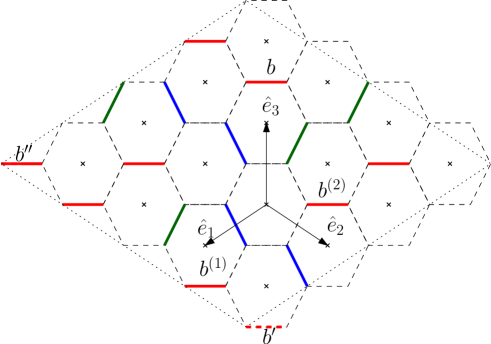
Figure 3. The hexagonal lattice $\mathcal{H}$ with the unit vectors $\hat{e}_{i},i=1,2,3$. The portion of $\mathcal{H}$ contained in the dotted region is the periodized lattice $\mathcal{H}_{L},L=4$. Crosses are vertices of the periodized triangular dual lattice $\mathcal{T}_{L}$. of $\mathcal{H}_{L}$. Thick edges are dimers of a perfect matching of $\mathcal{H}_{L}$ (the matching can be extended to a $4$-periodic perfect matching of the infinite lattice $\mathcal{H}$). Dimers are interlaced: for instance, type-3 (i.e., horizontal) dimers $b,b^{\prime}$ are interlaced with type-3 dimers $b^{(1)},b^{(2)}$. (Note that dimer $b^{\prime}$ is the same (by periodicity) as dimer $b^{\prime\prime}$; that is why it is drawn as dashed). In this drawing there are exactly $4$ dimers of types $1$ and $2$ and $8$ dimers of type $3$.

On $\mathcal{T}_{L}$ we introduce coordinates $u=(u_{1},u_{2})$ with $0\leq u_{i}\leq L-1$ by assigning coordinates $(0,0)$ to an arbitrarily fixed vertex of $\mathcal{T}_{L}$ (the “origin”) and letting $\hat{e}_{1},\hat{e}_{2}$ have coordinates $(1,0)$ and $(0,1)$ respectively. Note that the “unit vector” $\hat{e}_{3}$ has then coordinates $\hat{e}_{3}=(-1,-1)$.

The bipartite graph $\mathcal{H}_{L}$ has $2L^{2}$ vertices and every perfect matching $\eta$ of $\mathcal{H}_{L}$ contains exactly $L^{2}$ edges. Edges in a perfect matching $\eta$ are called dimers and $\eta$ is referred to as a dimer covering. We will say that an edge (or a dimer) is of type $i=1,2,3$ if it is parallel to the edge crossed by $\hat{e}_{i}$. The set $\Omega_{L}$ of all perfect matchings of $\mathcal{H}_{L}$ can be decomposed according to the number of dimers of the three types, as follows. Given $\bar{\rho}^{(L)}=(\bar{\rho}^{(L)}_{1},\bar{\rho}^{(L)}_{2})$ with $\bar{\rho}^{(L)}_{i}\in(0,1)$, $\sum_{i=1}^{2}\bar{\rho}_{i}^{(L)}\in(0,1)$ and $L\bar{\rho}^{(L)}_{i}\in\mathbb{N}$, let $\Omega_{\bar{\rho}^{(L)}}$ be the set of perfect matchings of $\mathcal{H}_{L}$ with $L^{2}\bar{\rho}^{(L)}_{i}$ dimers of type $i=1,2$. Note that the number of dimers of type $3$ is then constrained to be $L^{2}\bar{\rho}^{(L)}_{3}:=L^{2}(1-\bar{\rho}^{(L)}_{1}-\bar{\rho}^{(L)}_{2})$.

Let $\tau_{u}$ denote the translation by $u=(u_{1},u_{2})$. We recall a few known (and easy to verify) facts:

1. Given the locations of all dimers of a given type $i\in\{1,2,3\}$, the whole dimer covering $\eta$ is uniquely determined. In the following, we will call dimers of type $3$ (i.e. the horizontal ones) “particles”.

2. The positions of particles in a vertical column of hexagons are interlaced with those in the two neighboring columns. More explicitly, if there is a particle at a horizontal edge $b$ and another at the edge $b^{\prime}=\tau_{-n\hat{e}_{3}}b$ for some $n>0$ (note that $b,b^{\prime}$ are in the same column), then for $j=1,2$ there is a particle at an edge $b^{(j)}=\tau_{\hat{e}_{j}-r_{j}\hat{e}_{3}}b$, for some $r_{j}\in\{0,\dots,n-1\}$. See Figure 3 and 4. Similar interlacing conditions hold for dimers of types $1$ and $2$.

3. Every cycle of length $L$ on $\mathcal{T}_{L}$ in direction $\hat{e}_{i}$ crosses the same number of dimers of type $i$ (and therefore $L\bar{\rho}^{(L)}_{i}$ of them). This is a consequence of property (2).

We introduce a height function $H_{\eta}(\cdot)$ (defined on $\mathcal{T}_{L}$, i.e. on hexagonal faces of $\mathcal{H}_{L}$) for configurations $\eta\in\Omega_{\bar{\rho}^{(L)}}$. We first need some notation:

Definition 2.1.

Given $u\in\mathcal{T}_{L}$ and $i=1,2,3$, let $b_{i}(u)$ be the edge (necessarily of type $i$) of $\mathcal{H}_{L}$ that is crossed by the edge of $\mathcal{T}_{L}$ that joins $u$ to $u+\hat{e}_{i}$.

Then, we establish:

Definition 2.2 (Height function).

For every $\eta\in\Omega_{\bar{\rho}^{(L)}}$ we set $H_{\eta}(0,0)=0$ and

$$H_{\eta}(u+\hat{e}_{i})-H_{\eta}(u)=-\bar{\rho}^{(L)}_{i}+{\bf 1}_{b_{i}(u)\in\eta},\quad i=1,2,3.$$ (2.1)

The height function is well defined, i.e. the sum of the gradients along any closed cycle is zero. Indeed, when the cycle has trivial winding numbers around the torus $\mathcal{T}_{L}$ it suffices to verify that the total height change is zero along any elementary cycle of the type

$$u\to u+\hat{e}_{1}\to u+\hat{e}_{1}+\hat{e}_{2}\to u+\hat{e}_{1}+\hat{e}_{2}+\hat{e}_{3}=u.$$

In this case, the height change is

$$-\sum_{i=1,2,3}\bar{\rho}^{(L)}_{i}+{\bf 1}_{b_{1}(u)\in\eta}+{\bf 1}_{b_{2}(u+\hat{e}_{1})\in\eta}+{\bf 1}_{b_{3}(u+\hat{e}_{1}+\hat{e}_{2})\in\eta}=0$$

because exactly one of the three crossed edges, that share a common vertex, is occupied by a dimer and $\sum_{i=1,2,3}\bar{\rho}^{(L)}_{i}=1$. When instead the cycle winds once around $\mathcal{T}_{L}$ following direction $\hat{e}_{i}$, then the height change is zero because exactly $L\bar{\rho}^{(L)}_{i}$ dimers of type $i$ are crossed (property (3) above). The case of a general cycle easily follows.

Let $\mathbb{T}\subset\mathbb{R}^{2}$ be the open triangle of vertices $(0,0),(1,0),(0,1)$, so that $\bar{\rho}^{(L)}\in\mathbb{T}$. Assume that the sequence $\{\bar{\rho}^{(L)}\}_{L\in\mathbb{N}}$ converges to some $\bar{\rho}\in\mathbb{T}$ and that a sequence $\{\eta_{0}^{(L)}\}_{L\in\mathbb{N}}$ of configurations in $\Omega_{\bar{\rho}^{(L)}}$ approximates a smooth periodic function $\psi$, in the sense that

$$\lim_{L\to\infty}\frac{1}{L}H_{\eta_{0}^{(L)}}(\lfloor uL\rfloor)=\psi(u),\;\text{for every }u\in[0,1]^{2}.$$ (2.2)

Then, from the definition of height function we see that

$$\nabla\psi(u)+(\bar{\rho}_{1},\bar{\rho}_{2})\in\mathbb{T}\cup\partial\mathbb{T},\;\text{for every }u\in[0,1]^{2}.$$ (2.3)

2.2. The dynamics

We consider a Markov dynamics on $\Omega_{\bar{\rho}^{(L)}}$, that was introduced in [15] and later studied in [21] (in both these references, the dynamics is defined on the set of dimer coverings of a planar, rather than periodized, subset of $\mathcal{H}$). Also, with respect to [15, 21] we multiply transition rates by $L^{2}$, in order to avoid rescaling time in the hydrodynamic limit.

Recall from the previous section that the configuration $\eta$ is fully determined by the positions of the $L^{2}\bar{\rho}^{(L)}_{3}$ dimers of type $3$, or particles. The dynamics will be then defined directly in terms of particle moves.

Assign a label $p=1,\dots,L^{2}\bar{\rho}^{(L)}_{3}$ to particles. Given a configuration $\eta$ and a particle label $p$, let $I^{+}(p)\geq 0$ (resp. $I^{-}(p)\geq 0$) be the maximal displacement particle $p$ can take in direction $+\hat{e}_{3}$ (resp. $-\hat{e}_{3}$), without violating the interlacement constraints, when all other particles are kept fixed, cf. Fig. 4.

Figure 4. If particles $p_{1},\dots,p_{4}$ are kept fixed, then particle $p$ can be moved in direction $+\hat{e}_{3}$ (resp. $-\hat{e}_{3}$) by at most $2$ steps (resp. $1$ step). Therefore, $I^{+}(p)=2,I^{-}(p)=1$.

Definition 2.3 (Transition rates).

The possible updates of the dynamics are the following:

• a particle $p$ moves by $n\hat{e}_{3},0<n\leq I^{+}(p)$. This transition has rate $L^{2}/(2n)$.

• a particle $p$ moves by $-n\hat{e}_{3},0<n\leq I^{-}(p)$. This transition has also rate $L^{2}/(2n)$.

Observe that as soon as there are at least two particles in each cycle in direction $\hat{e}_{3}$ (which is certainly the case in our setting for $L$ large, since this number is $L\bar{\rho}^{(L)}_{3}$ and we assume that $\rho^{(L)}_{3}$ tends to a positive constant), a particle $p$ cannot reach the same position via a jump by $+n\hat{e}_{3},0<n\leq I^{+}(p)$ as with a jump by $-m\hat{e}_{3},0<m\leq I^{-}(p)$. Therefore, even if we are on the torus it makes sense to distinguish between “upward” and “downward” particle jumps.

The configuration at time $t$ will be denoted by $\eta(t)$ and the law of the process by $\mathbb{P}$. The uniform measure $\pi_{L}$ on $\Omega_{\bar{\rho}^{(L)}}$ is reversible (because transition rates are symmetric) and actually it is the unique stationary measure, since the Markov chain is ergodic (that any configuration in $\Omega_{\bar{\rho}^{(L)}}$ can be reached from any other via particle jumps of size $1$ is a classical argument [15] based on the definition of height function; for a proof in the periodized setting, see also [4, Lemma 1]).

We will formulate a hydrodynamic limit result for the height function. However, recall that only height increments are really defined by the particle configuration and one has to make a choice of an arbitrary global additive constant. In the definition of $H_{\eta}$ above we fixed such constant so that the height is zero at the origin. In the dynamical setting the natural choice is to fix the height at the origin to be the “integrated current at time $t$” (which is zero at initial time):

Definition 2.4 (Integrated current).

For $u\in\mathcal{T}_{L}$ and $t>0$ we define the integrated current $J(u,t)$ as the number of particles that cross $u$ downward minus the number of particles that cross $u$ upward in the time interval $[0,t]$. Also, we let

$$H(u,t)=H_{\eta_{0}}(u)+J(u,t).$$ (2.4)

Remark 2.5.

Note that $H(\cdot,t)$ is just the height function $H_{\eta(t)}$ (in the sense of Definition 2.2) of the configuration at time $t$, up to the global constant $H(0,t)=J(0,t)$. In particular, the analog of (2.1) holds at time $t$:

$$H(u+\hat{e}_{i},t)-H(u,t)=-\bar{\rho}^{(L)}_{i}+{\bf 1}_{b_{i}(u)\in\eta(t)}.$$ (2.5)

To understand the rationale behind Definition 2.4 note first of all that, in terms of dimer covering, moving a particle by $\pm\hat{e}_{3}$ corresponds to performing an elementary rotation of three dimers around a hexagonal face $u$ of $\mathcal{H}_{L}$. Say that $u$ is not the origin, where $H_{\eta}$ is fixed to zero. Then, according to Definition 2.2, the height at $u$ changes by $\mp 1$ as an effect of the rotation. Similarly, a move by $\pm m\hat{e}_{3}$ corresponds to the concatenation of $m$ rotations around $m$ adjacent, vertically stacked, hexagonal faces. See Figure 5. Correspondingly, when particle $p$ jumps by $\pm n\hat{e}_{3}$, the function $H(u,t)$ defined as in (2.4) changes by $\mp 1$ at the $n$ positions crossed by the particle.

Figure 5. A particle jump of length $n$ ($n=3$ here) corresponds to $n$ elementary dimer rotations in $n$ vertically stacked hexagonal faces.

2.3. Hydrodynamic limit

We assume that the initial condition of the dynamics approximates a smooth profile, in the sense of (2.2), but we impose a condition stronger than (2.3) on the gradient:

Assumption 2.6.

Let $\bar{\rho}=(\bar{\rho}_{1},\bar{\rho}_{2})\in\mathbb{T}$ be fixed. The initial condition $\eta_{0}=\eta_{0}^{(L)}$ belongs to $\Omega_{\bar{\rho}^{(L)}}$ and $\bar{\rho}^{(L)}\to\bar{\rho}$ as $L\to\infty$. Moreover, there exists a compact, convex subset $\mathcal{A}\subset\mathbb{T}$ and a periodic, $C^{2}$ function $\psi_{0}$ on the torus $[0,1]^{2}$ satisfying $\psi_{0}(0,0)=0$ and

$$\nabla\psi_{0}(u)+\bar{\rho}\in\mathcal{A},\quad\forall u\in[0,1]^{2}$$ (2.6)

such that (2.2) holds.

Our goal is to prove a hydrodynamic limit (in the diffusive scaling) for the height function $H$, under Assumption 2.6. See Remark 2.8 below for a discussion of whether such an assumption can be relaxed.

First, we define a function $W=(W_{1},W_{2}):\mathbb{T}\mapsto\mathbb{R}^{2}$ as

$$\begin{array}[]{ll}W_{1}(x,y)=-\frac{1}{2\pi}\cot(\pi(x+y))\sin^{2}(\pi y)-\frac{y}{4}+\frac{1}{4\pi}\sin(2\pi y)\\ W_{2}(x,y)=W_{1}(y,x).\end{array}$$ (2.7)

Our main result is the following:

Theorem 2.7.

Let $\eta_{0}=\{\eta_{0}^{(L)}\}_{L}$ satisfy Assumption 2.6. Then:

1. There exists a unique smooth solution of the Cauchy problem

   $$\left\{\begin{array}[]{l}\partial_{t}\psi(u,t)={\rm div}(W(\nabla\psi(u,t)+\bar{\rho})),\quad(u,t)\in[0,1]^{2}\times[0,\infty)\\ \psi(u,0)=\psi_{0}(u).\end{array}\right.$$ (2.10)

   The function $\psi$ is $C^{2,1}$ ($C^{2}$ in space and $C^{1}$ in time) and its gradient $\nabla\psi$ is continuous in time. Moreover, $\nabla\psi(u,t)+\bar{\rho}\in\mathcal{A}$ for every $u\in[0,1]^{2},t\geq 0$.

2. For every $t>0$

   $$\lim_{L\to\infty}D_{L}(t):=\lim_{L\to\infty}\frac{1}{L^{2}}\mathbb{E}\sum_{u\in\mathcal{T}_{L}}\left[\frac{H(u,t)}{L}-\psi\left(\frac{u}{L},t\right)\right]^{2}=0.$$ (2.11)

While it is not at first sight obvious that the PDE (2.10) is a parabolic equation, it was shown in [13, Sec. 3] that it can be equivalently rewritten as

$$\partial_{t}\psi=\mu(\nabla\psi+\bar{\rho})\sum_{i,j=1}^{2}\sigma_{i,j}(\nabla\psi+\bar{\rho})\frac{\partial^{2}}{\partial_{u_{i}}\partial_{u_{j}}}\psi$$ (2.12)

with $\mu(\cdot)>0$ and, for every $\rho\in\mathbb{T}$, $\{\sigma_{i,j}(\rho)\}_{i,j=1,2}$ a strictly positive-definite matrix, that is the Hessian of a strictly convex surface tension function. More precisely [13],

$$\mu(\rho)=\frac{1}{2\pi}\frac{\sin(\pi\rho_{1})\sin(\pi\rho_{2})}{\sin(\pi(1-\rho_{1}-\rho_{2}))}$$ (2.13)

while $\sigma_{i,j}(\rho)=\partial^{2}_{\rho_{i}\rho_{j}}\sigma(\rho)$,

$$\sigma(\rho)=\left\{\begin{array}[]{cc}\frac{1}{\pi}\left[\Lambda(\pi\rho_{1})+\Lambda(\pi\rho_{2})+\Lambda(\pi(1-\rho_{1}-\rho_{2}))\right]\leq 0,&\rho\in\mathbb{T}\cup\partial\mathbb{T}\\ +\infty&\quad\text{otherwise}\end{array}\right.$$ (2.16)

with

$$\Lambda(\theta)=\int_{0}^{\theta}\ln(2\sin(t))dt.$$

Note that $\sigma(\cdot)$ is the well-known surface tension for the dimer model on the hexagonal lattice as a function of the slope, cf. for instance [9, Sec. 7], and $-\Lambda(\cdot)$ is the so-called Lobachevsky function. Let us recall that, as well known and discussed for instance in [13, Sec. 3], $\sigma(\cdot)$ is $C^{\infty}$, strictly negative and strictly convex in $\mathbb{T}$, and note that $\mu(\cdot)$ is also $C^{\infty}$ and strictly positive in $\mathbb{T}$. Moreover, when $\rho$ approaches $\partial\mathbb{T}$ the function $\sigma(\rho)$ vanishes, the functions $\mu(\rho)$ and $\sigma_{i,j}(\rho)$ become singular and $\{\sigma_{i,j}\}_{i,j=1,2}$ loses the strict positive definiteness. Since however $\nabla\psi+\bar{\rho}$ stays in $\mathcal{A}\subset\mathbb{T}$ at all times, these potential singularities do not affect the solution of (2.12).

Remark 2.8.

Recall that the triangle $\mathbb{T}$ is open. Condition (2.6) means that we are requiring that $\nabla\psi_{0}+\bar{\rho}$ is uniformly away from $\partial\mathbb{T}$, the boundary of the set of allowed slopes. This is not just a technical assumption; indeed the coefficients $\mu(\cdot)$ and $\sigma_{i,j}(\cdot)$ of the hydrodynamic PDE (2.12) are singular on $\partial\mathbb{T}$ and it is not clear that its solution is well defined in general if (2.6) fails for the initial condition. On the other hand, the $C^{2}$ condition can certainly be relaxed, along the following lines. Assume $\psi_{0}$ is Lipschitz and satisfies (2.6); approximate it, within distance $\epsilon$ in sup norm, by $C^{2}$ functions $\psi^{\pm}$, with $\psi^{-}\leq\psi_{0}\leq\psi^{+}$, that verify (2.6) for some compact sets $\mathcal{A}^{\pm}$, close to $\mathcal{A}$ in Hausdorff distance. Theorem 2.7 holds for initial conditions $\eta_{0}^{\pm}$ that tend to $\psi^{\pm}$; since the dynamics is attractive, i.e. preserves stochastic ordering between height profiles, the hydrodynamic limit for initial condition $\eta_{0}$ can be obtained by letting $\epsilon\to 0$ after $L\to\infty$. To avoid overloading this work, we prefer not to work out in full detail the argument we just outlined, and to state the main result under the $C^{2}$ assumption.

2.4. Short sketch of the proof of the main Theorem

The proof of item (ii) of Theorem 2.7 is the object of Sections 4 to 6 and, in its general lines, follows the ideas of the $H^{-1}$ norm method as in [7]. The point is to study

$$D_{L}(t)-D_{L}(0)$$ (2.17)

and to show that it is non-positive in the $L\to\infty$ limit. The first step, accomplished in Section 4, is to note that one can rewrite (2.17) as the average, with respect to certain space-time averaged limiting measures $\nu_{t,(i,j)}$, of a function depending only on the local gradients of $H$ and of $\psi$. This step would not be possible e.g. for the single-flip Glauber dynamics, and the fact that it works in our case is the signature of the above-mentioned “gradient condition”. The second step, in Section 5, is to argue that the measures $\nu_{t,(i,j)}$ have to be translation invariant Gibbs measures because of a general entropy production argument. This allows us to rewrite them as some linear combinations of ergodic, translation invariant measures with (unknown) density $w_{\nu_{t(i,j)}}$. Finally, in Section 6, thanks to the exact solvability of the uniform dimer covering model, we rewrite (2.17) as an explicit function of the density $w_{\nu_{t,(i,j)}}$. A non-trivial algebraic identity then implies that this function is non-positive independently of $w_{\nu_{t,(i,j)}}$, which concludes the proof. This identity is related to the fact that the limit PDE contracts the $\mathbb{L}^{2}$ distance which, as we mentioned in the introduction, is also a remarkable and a-priori not obvious property of our model.

3. The limit PDE

Item (i) in Theorem 2.7 is a consequence of rather classical results in the theory of non-linear parabolic PDEs, cf. for instance [14]. We still discuss it briefly, mostly to show why the fact that the coefficients of the equation are singular on the boundary of $\mathbb{T}$ does not affect the regularity of the solution.

Consider the Cauchy problem

$$\left\{\begin{array}[]{l}\partial_{t}\phi=\kappa(\nabla\phi)\sum_{i,j=1}^{2}g_{i,j}(\nabla\phi)\frac{\partial^{2}}{\partial_{u_{i}}\partial_{u_{j}}}\phi,\;u\in[0,1]^{2},t\geq 0\\ \phi(u,0)=\phi_{0}(u),\end{array}\right.$$ (3.3)

where $\phi_{0}(\cdot)$ is a $C^{2}$ periodic function on $[0,1]^{2}$. Here, $\kappa(\cdot)$ is a strictly positive and $C^{\infty}$ function on $\mathbb{R}^{2}$, while $g_{i,j}(x)=\partial^{2}_{x_{i}x_{j}}g(x)$, for a strictly convex, $C^{\infty}$ function $g:\mathbb{R}^{2}\to\mathbb{R}$. We further assume that, letting $g^{(2)}(x):=\{g_{i,j}(x)\}_{i,j=1,2}$, one has

$$c_{-}\mathbb{I}\leq g^{(2)}(x),$$

with $\mathbb{I}$ the $2\times 2$ identity matrix and $c_{-}>0$ and, finally, that

$$|p|^{3}|Dg_{i,j}(p)|\stackrel{{\scriptstyle|p|\to\infty}}{{=}}O(|p|^{2})$$

with $Dg_{i,j}$ the gradient of $g_{i,j}$. Then, it is known (see [14, Th. 12.16] and the remarks following it) that (3.3) admits a unique global classical solution $\phi$ that belongs to a certain Hölder space $H_{a},a>2$ and in particular that $\phi$ is at least $C^{2}$ in space, $C^{1}$ in time and its gradient $\nabla\phi$ is continuous in time (in reality, using the $C^{\infty}$ regularity of the coefficients of the equation one may bootstrap the argument to get $C^{\infty}$ regularity for $\phi$, but we do not need this).

Assume that $\phi_{0}$ satisfies the same condition as $\psi_{0}$ in (2.6). A standard comparison argument gives that $\phi(\cdot,t)$ still satisfies (2.6) at all later times. Namely, write the convex set $\mathcal{A}-\bar{\rho}$ (the translation of $\mathcal{A}$ by $-\bar{\rho}$) as the intersection of half-planes:

$$\mathcal{A}-\bar{\rho}=\cap_{n\in\mathbb{S}^{1}}\{x\in\mathbb{R}^{2}:x\cdot n\leq f(n)\}$$ (3.4)

and for any $n\in\mathbb{S}^{1},a>0$ define

$$\hat{\phi}(u,t):=\phi(u+na,t)-af(n),$$

which is still a smooth solution of (3.3), this time with initial condition $\phi_{0}(\cdot+na)-af(n)$. Since at time zero $\hat{\phi}\leq\phi$, by the maximum principle the same holds at later times and therefore $\nabla\phi(u,t)+\bar{\rho}\in\mathcal{A}$.

Now let us go back to our PDE (2.10) and let us recall that it is equivalent to (2.12). Define $g:\mathbb{R}^{2}\mapsto\mathbb{R}$ and $\kappa:\mathbb{R}^{2}\mapsto\mathbb{R}$ such that $g$ and $\kappa$ coincide with $\sigma$ and $\mu$ respectively on $\mathcal{A}$, while at the same time $g$ and $\kappa$ satisfy the smoothness and convexity/positivity assumptions formulated just after (3.3). From the discussion above we know that the solution of the Cauchy problem (3.3) with $\phi_{0}\equiv\psi_{0}$ is smooth and $\nabla\phi(u,t)\in\mathcal{A}$ for every $u,t$. Since $g\equiv\sigma$ and $\kappa\equiv\mu$ in $\mathcal{A}$, we deduce that $\phi$ also solves (2.12) (and therefore (2.10)).

4. Computation of $D_{L}(t)$ in terms of limit measures

We start the bulk of the work, i.e. the proof of claim (ii) of Theorem 2.7. The goal of this section is to prove the upper bound (4.58) for $\limsup_{L}D_{L}(t)$ in terms of certain space-time averaged measures $\nu_{t,(i,j)}$.

4.1. Some preliminary definitions

We need some notation: given a function $f:\mathcal{T}_{L}\to\mathbb{R}$ we let

$$\hat{\nabla}_{i}f(u)=f(u)-f(u-\hat{e}_{i}),i=1,2$$

and $\hat{\nabla}f(u)=(\hat{\nabla}_{1}f(u),\hat{\nabla}_{2}f(u))$. Moreover, given $\eta\in\Omega_{\bar{\rho}^{(L)}}$ and $u\in\mathcal{T}_{L}$, we let

$$\epsilon(u,\eta)={\bf 1}_{\{b_{1}(u),b_{2}(u)\}\subset\eta}-{\bf 1}_{\{b_{1}(u-\hat{e}_{1}),b_{2}(u-\hat{e}_{2})\}\subset\eta}\in\{0,-1,+1\},$$ (4.1)

with $b_{i}(u)$ as in Definition 2.1. It is immediately seen that the events

$$\{b_{1}(u),b_{2}(u)\}\subset\eta$$

and

$$\{b_{1}(u-\hat{e}_{1}),b_{2}(u-\hat{e}_{2})\}\subset\eta$$

are mutually exclusive.

For any vertex $u\in\mathcal{T}_{L}$ such that $\epsilon(u,\eta)\neq 0$, we define

$$k(u,\eta)=\max\{n\geq 1:\epsilon(u+(n-1)\epsilon(u,\eta)\hat{e}_{3},\eta)=\epsilon(u,\eta)\}\geq 1.$$ (4.2)

Note that, if $\epsilon(u,\eta)=+1$ (resp. if $\epsilon(u,\eta)=-1$) then $k(u,\eta)$ is the smallest integer such that there is a dimer of type $3$ at $b_{3}(u+(n-1)\hat{e}_{3})$ (resp. at $b_{3}(u-n\hat{e}_{3})$). See Fig. 6.

Figure 6. (a): here, $\epsilon(u,\eta)=+1$ and $k=k(u,\eta)=3$ since $k$ is the smallest integer such that $\epsilon(u+(k-1)\hat{e}_{3},\eta)=1$ while $\epsilon(u+k\hat{e}_{3},\eta)\neq 1$. (b): in this case, $\epsilon(u,\eta)=-1$ and $k=k(u,\eta)=2$.

For later convenience, it is useful to remark the following:

Lemma 4.1.

For every configuration $\eta\in\Omega_{\bar{\rho}^{(L)}}$ and $u\in\mathcal{T}_{L}$, one has the identity

$$\epsilon(u,\eta)=\frac{1}{2}\left[F(u+\hat{e}_{3},\eta)-F(u,\eta)+\Delta H_{\eta}(u)\right]$$ (4.3)

where

$$\Delta H_{\eta}(u)=\sum_{i=1}^{2}\left[H_{\eta}(u+\hat{e}_{i})+H_{\eta}(u-\hat{e}_{i})\right]-4H_{\eta}(u)$$ (4.4)

$$=\hat{\nabla}_{1}(\hat{\nabla}_{1}H_{\eta})(u+\hat{e}_{1})+\hat{\nabla}_{2}(\hat{\nabla}_{2}H_{\eta})(u+\hat{e}_{2})$$ (4.5)

and

$$F(u,\eta)=|{\bf 1}_{b_{1}(u)\in\eta}-{\bf 1}_{b_{2}(u)\in\eta}|.$$ (4.6)

Note that, while $\mathcal{T}$ is the triangular lattice, $\Delta$ in (4.4) is the ordinary $\mathbb{Z}^{2}$ Laplacian with respect to the coordinate axes $\hat{e}_{1},\hat{e}_{2}$.

Proof of Lemma 4.1.

Note first of all the trivial identities

$$|{\bf 1}_{b\in\eta}-{\bf 1}_{b^{\prime}\in\eta}|={\bf 1}_{b\in\eta}+{\bf 1}_{b^{\prime}\in\eta}-2{\bf 1}_{\{b,b^{\prime}\}\subset\eta}$$ (4.7)

and

$$\Delta H_{\eta}(u)=({\bf 1}_{b_{1}(u)\in\eta}-{\bf 1}_{b_{1}(u-\hat{e}_{1})\in\eta})+({\bf 1}_{b_{2}(u)\in\eta}-{\bf 1}_{b_{2}(u-\hat{e}_{2})\in\eta}).$$ (4.8)

Then, the r.h.s. of (4.3) equals

$$\frac{1}{2}|{\bf 1}_{b_{1}(u+\hat{e}_{3})\in\eta}-{\bf 1}_{b_{2}(u+\hat{e}_{3})\in\eta}|-\frac{1}{2}({\bf 1}_{b_{1}(u)\in\eta}+{\bf 1}_{b_{2}(u)\in\eta}-2{\bf 1}_{\{b_{1}(u),b_{2}(u)\}\subset\eta})\\ +\frac{1}{2}({\bf 1}_{b_{1}(u)\in\eta}-{\bf 1}_{b_{1}(u-\hat{e}_{1})\in\eta})+\frac{1}{2}({\bf 1}_{b_{2}(u)\in\eta}-{\bf 1}_{b_{2}(u-\hat{e}_{2})\in\eta})$$ (4.9)

and using (4.7) again for $b=b_{1}(u-\hat{e}_{1}),b^{\prime}=b_{2}(u-\hat{e}_{2})$, we obtain

$${\bf 1}_{\{b_{1}(u),b_{2}(u)\}\subset\eta}-{\bf 1}_{\{b_{1}(u-\hat{e}_{1}),b_{2}(u-\hat{e}_{2})\}\subset\eta}\\ +\frac{1}{2}\left[|{\bf 1}_{b_{1}(u+\hat{e}_{3})\in\eta}-{\bf 1}_{b_{2}(u+\hat{e}_{3})\in\eta}|-|{\bf 1}_{b_{1}(u-\hat{e}_{1})\in\eta}-{\bf 1}_{b_{2}(u-\hat{e}_{2})\in\eta}|\right].$$ (4.10)

The first line of (4.10) is exactly $\epsilon(u,\eta)$ and the second line is identically zero (this is easily checked in all the finitely many allowed dimer configurations of edges $b_{1}(u+\hat{e}_{3}),b_{2}(u+\hat{e}_{3}),b_{1}(u-\hat{e}_{1}),b_{2}(u-\hat{e}_{2}),b_{3}(u)$). ∎

4.2. Computation of $d/dtD_{L}(t)$

By our assumption on the initial condition we know that (2.11) holds for $t=0$. Then, we differentiate $D_{L}(t)$ with respect to $t$ and integrate back with the hope that, for every $t>0$,

$$\limsup_{L\to\infty}\int_{0}^{t}ds\,\frac{d}{ds}D_{L}(s)\leq 0.$$ (4.11)

We first notice that the time derivative of $D_{L}(t)$ can be written as the sum of four terms:

$$\frac{d}{dt}D_{L}(t)=\sum_{i=1}^{4}B_{i}(t)$$ (4.12)

$$B_{1}(t)=\frac{d}{dt}\frac{1}{L^{2}}\mathbb{E}\sum_{u\in\mathcal{T}_{L}}\frac{H^{2}(u,t)}{L^{2}}$$ (4.13)

$$B_{2}(t)=-\frac{2}{L^{2}}\sum_{u\in\mathcal{T}_{L}}\psi(u/L,t)\frac{d}{dt}\mathbb{E}\frac{H(u,t)}{L}$$ (4.14)

$$B_{3}(t)=-\frac{2}{L^{2}}\sum_{u\in\mathcal{T}_{L}}\mathbb{E}\frac{H(u,t)}{L}\partial_{t}\psi(u/L,t)$$ (4.15)

$$B_{4}(t)=\frac{2}{L^{2}}\sum_{u\in\mathcal{T}_{L}}\psi(u/L,t)\partial_{t}\psi(u/L,t).$$ (4.16)

We put $\Psi(u,t):=L\psi(u/L,t)$, with $u\in\mathcal{T}_{L}$ and $\psi$ the solution of (2.10). Then we re-express each $B_{i}(t)$ using the definition of the transition rates:

Proposition 4.2.

$$B_{1}(t)=\frac{1}{L^{2}}\mathbb{E}\sum_{u\in\mathcal{T}_{L}}\left(\frac{|\epsilon(u,t)|}{2}-\bar{\rho}_{3}^{(L)}|\epsilon(u,t)|\frac{k(u,t)-1}{2}+\epsilon(u,t)H(u,t)\right)$$ (4.17)

$$B_{2}(t)=-\frac{1}{L^{2}}\sum_{u\in\mathcal{T}_{L}}\mathbb{E}\left\{\Psi\left(u,t\right)\epsilon(u,t)+\frac{\epsilon(u,t)}{k(u,t)}\sum_{j=0}^{k(u,t)-1}\left[\Psi\left(u+j\epsilon(u,t)\hat{e}_{3}\right)-\Psi\left(u,t\right)\right]\right\}$$ (4.18)

$$B_{3}(t)=\frac{2}{L^{2}}\sum_{u\in\mathcal{T}_{L}}W(\hat{\nabla}\Psi(u,t)+\bar{\rho})\cdot\mathbb{E}\hat{\nabla}H(u,t)+o(1)$$ (4.19)

$$B_{4}(t)=-\frac{2}{L^{2}}\sum_{u\in\mathcal{T}_{L}}\hat{\nabla}\Psi(u,t)\cdot W(\hat{\nabla}\Psi(u,t)+\bar{\rho})+o(1)$$ (4.20)

where the error terms $o(1)$ tend to zero as $L\to\infty$, uniformly on compact time intervals, and $k(u,t),\epsilon(u,t)$ are short-hand notations for $k(u,\eta(t)),$ $\epsilon(u,\eta(t))$.

Proof of Proposition 4.2.

We remark that, if a particle $p$ moves downward to an edge $b$ and $u\in\mathcal{T}_{L}$ is the unique vertex such that $b=b_{3}(u-\hat{e}_{3})$, then necessarily $\epsilon(u,\eta)=+1$. Similarly, if a particle $p$ moves upward to an edge $b$ and $u\in\mathcal{T}_{L}$ is the unique vertex such that $b=b_{3}(u)$, then necessarily $\epsilon(u,\eta)=-1$. In both cases the length of such a jump is exactly $k(u,\eta)$, so that the jump occurs with rate $L^{2}/(2k(u,\eta))$, and (see Remark 2.5) the height function $H$ changes by $\epsilon(u,\eta)$ at faces labelled $u+j\epsilon(u,\eta)\hat{e}_{3}$, $j=0,\dots,k(\epsilon,\eta)-1$.

One deduces then

$$B_{1}(t)=\frac{1}{L^{2}}\sum_{u\in\mathcal{T}_{L}}\mathbb{E}\frac{|\epsilon(u,t)|}{2k(u,t)}\sum_{j=0}^{k(u,t)-1}\Bigl{[}\left(H(u+j\epsilon(u,t)\hat{e}_{3},t)+\epsilon(u,t)\right)^{2}\\ -H(u+j\epsilon(u,t)\hat{e}_{3},t)^{2}\Bigr{]}\\ =\frac{1}{L^{2}}\sum_{u\in\mathcal{T}_{L}}\mathbb{E}\frac{|\epsilon(u,t)|}{2k(u,t)}\sum_{j=0}^{k(u,t)-1}\left(2\epsilon(u,t)H(u+j\epsilon(u,t)\hat{e}_{3},t)+1\right),$$ (4.21)

where the factor $|\epsilon(u,t)|$ is there to select those $u$ for which $\epsilon(u,t)\neq 0$ and a transition is possible. On the other hand,

$$H(u+j\epsilon(u,t)\hat{e}_{3},t)=H(u,t)-j\bar{\rho}^{(L)}_{3}\epsilon(u,t)\;\text{for every }j=0,\ldots,k(u,t)-1$$

as follows from (2.5) for $i=3$, since no horizontal dimer is crossed by the vertical path from $u$ to $u+\epsilon(u,t)(k(u,t)-1)\hat{e}_{3}$. Therefore, summing over $j$, one finds (4.17) as desired.

Similarly,

$$B_{2}(t)=-\frac{2}{L^{2}}\sum_{u\in\mathcal{T}_{L}}\mathbb{E}\frac{|\epsilon(u,t)|}{2k(u,t)}\sum_{j=0}^{k(u,t)-1}\epsilon(u,t)\Psi(u+j\epsilon(u,t)\hat{e}_{3},t)$$ (4.22)

which is the same as (4.18).

As for (4.19), just note that

$$B_{3}(t)=-\frac{2}{L^{2}}\sum_{u\in\mathcal{T}_{L}}\mathbb{E}\frac{H(u,t)}{L}\left.{\rm div}(W(\nabla\psi+\bar{\rho}))\right|_{(u/L,t)}.$$ (4.23)

Since $\psi$ is $C^{2}$ in space and using also $\nabla\psi(\cdot,t)\in\mathcal{A}\subset\mathbb{T}$ and smoothness of $W$ in $\mathbb{T}$, we have

$$\left.{\rm div}(W(\nabla\psi+\bar{\rho}))\right|_{(u/L,t)}=o(1)+L\sum_{j=1}^{2}\hat{\nabla}_{j}W_{j}(\hat{\nabla}\Psi+\bar{\rho}){(u,t)}$$ (4.24)

where the error term is uniform over all finite time intervals. Note that the second term in the r.h.s. of (4.24) is $O(1)$ and not $O(L)$, because the discrete gradient $\hat{\nabla}_{j}$ is essentially $1/L$ times the continuous gradient. A discrete summation by parts then gives

$$B_{3}(t)=\frac{2}{L^{2}}\sum_{u\in\mathcal{T}_{L}}\mathbb{E}\hat{\nabla}H(u,t)\cdot W(\hat{\nabla}\Psi(u,t)+\bar{\rho})$$ (4.25)

$$+o(1)\times\frac{1}{L^{2}}\sum_{u\in\mathcal{T}_{L}}\mathbb{E}\frac{H(u,t)}{L}.$$ (4.26)

In order to get (4.19) it suffices to prove that the sum multiplying $o(1)$ is of order $1$ with respect to $L$, uniformly on finite time intervals. In fact, one has even more: the sum in question does not depend on time at all (and at time zero it is $O(1)$ because by definition the height function is bounded by $L$). Indeed, the same steps that led to (4.18) give

$$\frac{d}{dt}\frac{1}{L^{2}}\sum_{u\in\mathcal{T}_{L}}\mathbb{E}\frac{H(u,t)}{L}=\frac{1}{2L}\sum_{u\in\mathcal{T}_{L}}\mathbb{E}\epsilon(u,t)$$ (4.27)

(one just needs to replace $-2\psi(\cdot,\cdot)$ by the constant $1$ in (4.18)). Using Lemma 4.1 and summation by parts, the r.h.s. of (4.27) is immediately seen to be zero.

Finally, the proof of (4.20) is simpler than that of (4.19) (it uses only smoothness of the solution of the PDE and summation by parts, while the Markov process does not appear) and is left to the reader. ∎

Note that all terms in the sums defining $B_{1}(t),\dots,B_{4}(t)$ are of order $1$ (we will see later that $k(u,t)$ is typically $O(1)$, see Proposition 4.8), except for $\epsilon(u,t)H(u,t)$ and $\epsilon(u,t)\Psi(u,t)$, that a priori are of order $L$. However, the spatial sum of these terms can be rewritten in a more convenient form, from which it is clear that it is of the good order of magnitude:

Proposition 4.3.

One has the following identities:

$$\sum_{u\in\mathcal{T}_{L}}\epsilon(u,t)H(u,t)\\ =\frac{\bar{\rho}^{(L)}_{3}}{2}\sum_{u\in\mathcal{T}_{L}}F(u,\eta(t))-\frac{1}{2}\sum_{u\in\mathcal{T}_{L}}\left((\hat{\nabla}_{1}H(u,t))^{2}+(\hat{\nabla}_{2}H(u,t))^{2}\right)$$ (4.28)

and

$$\sum_{u\in\mathcal{T}_{L}}\epsilon(u,t)\Psi(u,t)=\frac{1}{2}\sum_{u\in\mathcal{T}_{L}}F(u,\eta(t))(\hat{\nabla}_{1}\Psi(u,t)+\hat{\nabla}_{2}\Psi(u,t))\\ -\frac{1}{2}\sum_{u\in\mathcal{T}_{L}}\left(\hat{\nabla}_{1}H(u,t)\hat{\nabla}_{1}\Psi(u,t)+\hat{\nabla}_{2}H(u,t)\hat{\nabla}_{2}\Psi(u,t)\right)+o(L^{2})$$ (4.29)

where $F(u,\eta)$ was defined in (4.6) and $o(L^{2})$ is uniform on bounded time intervals.

Proof of Proposition 4.3.

Let us show the first identity (4.28). We have, from Lemma 4.1 and a summation by parts,

$$\sum_{u\in\mathcal{T}_{L}}\epsilon(u,t)H(u,t)\\ =\frac{1}{2}\sum_{u\in\mathcal{T}_{L}}\left[F(u+\hat{e}_{3},\eta(t))-F(u,\eta(t))+\sum_{j=1,2}\hat{\nabla}_{j}\hat{\nabla}_{j}H(u+\hat{e}_{j},t)\right]H(u,t)\\ =-\frac{1}{2}\sum_{u\in\mathcal{T}_{L}}\left[F(u,\eta(t))(H(u,t)-H(u-\hat{e}_{3},t))+\hat{\nabla}H(u,t)\cdot\hat{\nabla}H(u,t)\right].$$ (4.30)

Next, recall (4.7) and (cf. (2.5))

$$H(u,t)-H(u-\hat{e}_{3},t)={\bf 1}_{b_{3}(u-\hat{e}_{3})\in\eta(t)}-\bar{\rho}^{(L)}_{3}.$$ (4.31)

Since the event $\{b_{3}(u-\hat{e}_{3})\in\eta\}$ is incompatible with both $\{b_{1}(u)\in\eta\}$ and $\{b_{2}(u)\in\eta\}$ (the two events appearing in the definition of $F(u,\eta)$), the indicator function ${\bf 1}_{b_{3}(u-\hat{e}_{3})\in\eta(t)}$ in (4.31) can be omitted and (4.28) follows.

The proof of (4.29) is analogous. The error term $o(L^{2})$ comes from approximating

$$\Psi(u-\hat{e}_{3},t)-\Psi(u,t)=\hat{\nabla}_{1}\Psi(u,t)+\hat{\nabla}_{2}\Psi(u,t)+o(1).$$

∎

Altogether, given that

$$\hat{\nabla}_{i}H(u,t)={\bf 1}_{b_{i}(u-\hat{e}_{i})\in\eta(t)}-\bar{\rho}^{(L)}_{i},\;i=1,2$$ (4.32)

we have obtained:

Proposition 4.4.

$$B_{i}(t)=\frac{1}{L^{2}}\mathbb{E}\sum_{u\in\mathcal{T}_{L}}C_{i}(\eta_{-u}(t),\Psi_{-u}(t))+o(1)$$ (4.33)

where $\eta_{-u}$ and $\Psi_{-u}$ denote the configurations $\eta$ and $\Psi$ translated by $-u$, $o(1)$ is uniform on bounded time intervals and we set

$$C_{1}(\eta,\Psi(t)):=C_{1}(\eta)=\frac{|\epsilon(0,\eta)|}{2}-\bar{\rho}^{(L)}_{3}|\epsilon(0,\eta)|\frac{k(0,\eta)-1}{2}+\frac{\bar{\rho}_{3}}{2}F(0,\eta)$$ (4.34)

$$-\frac{1}{2}\left({\bf 1}_{b_{1}(0)\in\eta}(1-2\bar{\rho}_{1})+\bar{\rho}_{1}^{2}+{\bf 1}_{b_{2}(0)\in\eta}(1-2\bar{\rho}_{2})+\bar{\rho}_{2}^{2}\right)$$

$$C_{2}(\eta,\Psi(t))=-\frac{\epsilon(0,\eta)}{k(0,\eta)}\sum_{j=0}^{k(0,\eta)-1}\left[\Psi\left(j\epsilon(0,\eta)\hat{e}_{3},t\right)-\Psi\left(0,t\right)\right]$$ (4.35)

$$\quad-\frac{1}{2}F(0,\eta)(\hat{\nabla}_{1}\Psi(0,t)+\hat{\nabla}_{2}\Psi(0,t))$$

$$\quad+\frac{1}{2}\left(({\bf 1}_{b_{1}(0)\in\eta}-\bar{\rho}_{1})\hat{\nabla}_{1}\Psi(0,t)+({\bf 1}_{b_{2}(0)\in\eta}-\bar{\rho}_{2})\hat{\nabla}_{2}\Psi(0,t)\right)$$

$$C_{3}(\eta,\Psi(t))=2W(\hat{\nabla}\Psi(0,t)+\bar{\rho})\cdot({\bf 1}_{b_{1}(0)\in\eta}-\bar{\rho}_{1},{\bf 1}_{b_{2}(0)\in\eta}-\bar{\rho}_{2})$$ (4.36)

$$C_{4}(\eta,\Psi(t))=-2\hat{\nabla}\Psi(0,t)\cdot W(\hat{\nabla}\Psi(0,t)+\bar{\rho}).$$ (4.37)

The error terms $o(1)$ come from those in Propositions 4.2 and 4.3, and also from harmless approximations of the type

$$\bar{\rho}^{(L)}_{i}=\bar{\rho}_{i}+o(1),\quad\hat{\nabla}_{j}\Psi(u,t)=\hat{\nabla}_{j}\Psi(u-\hat{e}_{j},t)+o(1).$$ (4.38)

Note that $C_{i}(\eta,\Psi(t))$ depends only on the gradients of $\Psi(t)$ (similarly, $C_{i}$ depends on $\eta$, i.e. on the gradients of the height function associated to $\eta$). Actually, $C_{1}$ is independent of $\Psi$ and $C_{4}$ is independent of $\eta$, while $C_{2},C_{3}$ depend non-trivially on both variables. Also observe that only the $C_{1}$ term depends explicitly on $L$, through the term $\bar{\rho}^{(L)}_{3}|\epsilon(0,\eta)|\frac{k(0,\eta)-1}{2}$.

Recall that we want to prove (4.11). Integrating $d/dsD_{L}(s)$ from time $0$ to time $t$, we find from Proposition 4.4

$$D_{L}(t)=D_{L}(0)+\frac{t}{L^{2}}\sum_{u\in\mathcal{T}_{L}}\frac{1}{t}\int_{0}^{t}\mathbb{E}\sum_{i=1}^{4}C_{i}(\eta_{-u}(s),\Psi_{-u}(s))\,\mathrm{d}s+o(1).$$ (4.39)

This expression involves a triple average on space, time and on the realization of the process. Recall also that, while we do not indicate this explicitly, both the law $\mathbb{E}$ and the function $\Psi(\cdot,s)$ depend on $L$.

Let $\Omega$ be the set of all dimer coverings of $\mathcal{H}$. We put the product topology on $\Omega$, which makes it compact: as a metric we can take for instance

$$d(\eta,\eta^{\prime})=\sum_{e\in\mathcal{H}}2^{-|e|}|{\bf 1}_{e\in\eta}-{\bf 1}_{e\in\eta^{\prime}}|$$

where the sum over $e$ runs over all edges of $\mathcal{H}$ and $|e|$ is the distance between $e$ and the origin. Given this, we observe that

$$\sum_{i=1}^{4}C_{i}(\eta,\Psi(s))=C(\eta,\Psi(s))+U^{(L)}(\eta,\Psi(s))$$

where $C(\eta,\Psi(s))$ is a bounded and continuous function on $\Omega$ while $U^{(L)}(\eta,\Psi(s))$ is the unbounded term

$$U^{(L)}(\eta,\Psi(s))$$ (4.40)

$$=-\bar{\rho}^{(L)}_{3}|\epsilon(0,\eta)|\frac{k(0,\eta)-1}{2}-\frac{\epsilon(0,\eta)}{k(0,\eta)}\sum_{j=0}^{k(0,\eta)-1}\left[\Psi\left(j\epsilon(0,\eta)\hat{e}_{3},s\right)-\Psi\left(0,s\right)\right].$$

Note in particular that, as indicated by the notation, there is no dependence on $L$ in the function $C$. The function $U^{(L)}(\eta,\Psi(s))$ instead depends explicitly on $L$ through $\bar{\rho}^{(L)}_{3}$. The goal of the rest of this section is to replace $U^{(L)}$ with a bounded, continuous and $L$-independent function $U_{M}$, where $M$ is a cut-off parameter that will be sent to infinity at the very end.

First of all we claim:

Lemma 4.5.

One has $U^{(L)}(\eta,\Psi(s))\leq 0$ as soon as $L$ is larger than some $L_{0}$ independent of $\eta,s$.

Proof of Lemma 4.5.

We can assume that $\epsilon(0,\eta)=\pm 1$: indeed, if $\epsilon(0,\eta)=0$ then $U^{(L)}(\eta,\Psi(s))=0$ and there is nothing to prove. Since $\nabla\psi(u,t)+\bar{\rho}\in\mathcal{A}$ for every $u\in[0,1]^{2},t\geq 0$, we know that $\Psi(t)$ satisfies

$$\left\{\begin{array}[]{ll}\delta\leq\hat{\nabla}_{i}\Psi(u,t)+\bar{\rho}_{i}\leq 1-\delta,&i=1,2,\\ \delta\leq\hat{\nabla}_{1}\Psi(u,t)+\hat{\nabla}_{2}\Psi(u,t)+\bar{\rho}_{1}+\bar{\rho}_{2}\leq 1-\delta&,\end{array}\right.$$ (4.43)

for some $\delta>0$ independent of $t,u$. Therefore,

$$-\epsilon(0,\eta)\left[\Psi\left(j\epsilon(0,\eta)\hat{e}_{3},s\right)-\Psi\left(0,s\right)\right]\leq j(1-\delta-\bar{\rho}_{1}-\bar{\rho}_{2})$$ (4.44)

$$=|\epsilon(0,\eta)|j(\bar{\rho}_{3}-\delta).$$ (4.45)

Summing over $j$, the r.h.s. of (4.40) is upper bounded by

$$-|\epsilon(0,\eta)|\frac{k(0,\eta)-1}{2}(\bar{\rho}^{(L)}_{3}-\bar{\rho}_{3}+\delta)$$ (4.46)

which is negative for $L$ large enough given that $\bar{\rho}^{(L)}_{3}\to\bar{\rho}_{3}$. ∎

As a consequence, for every $M>0$ and assuming $L>L_{0}$ we have

$$U^{(L)}(\eta,\Psi(s))\leq U^{(L)}(\eta,\Psi(s)){\bf 1}_{|\epsilon(0,\eta)|k(0,\eta)\leq M}=U_{M}(\eta,\Psi(s))+\delta_{L}(M)$$ (4.47)

where

$$U_{M}(\eta,\Psi(s))=U(\eta,\Psi(s)){\bf 1}_{|\epsilon(0,\eta)|k(0,\eta)\leq M},$$ (4.48)

with $U(\eta,\Psi(s))$ defined as $U^{(L)}(\eta,\Psi(s))$ except that $\bar{\rho}^{(L)}$ is replaced by $\bar{\rho}$, while

$$\delta_{L}(M)=(\bar{\rho}_{3}-\bar{\rho}^{(L)}_{2})|\epsilon(0,\eta)|\frac{k(0,\eta)-1}{2}{\bf 1}_{|\epsilon(0,\eta)|k(0,\eta)\leq M}$$

so that $|\delta_{L}(M)|\leq|\bar{\rho}_{3}-\bar{\rho}^{(L)}_{2}|M$ which tends to zero as $L\to\infty$ (not uniformly in $M$). Note that $U_{M}$ is continuous in $\eta$. Indeed, the mapping

$$\eta\mapsto M\wedge|\epsilon(0,\eta)|k(0,\eta)$$

is continuous (its value is determined by the configuration of $\eta$ in a window of size $M$ around the origin).

Altogether, we have obtained:

Proposition 4.6.

As soon as $L\geq L_{0}$, we have for every $M>0$

$$D_{L}(t)\leq D_{L}(0)+\delta_{L}(M)\\ +\frac{t}{L^{2}}\sum_{u\in\mathcal{T}_{L}}\frac{1}{t}\int_{0}^{t}\mathbb{E}\left[C(\eta_{-u}(s),\Psi_{-u}(s))+U_{M}(\eta_{-u}(s),\Psi_{-u}(s))\right]\,\mathrm{d}s.$$ (4.49)

The functions $C(\cdot,\Psi(t))$ and $U_{M}(\cdot,\Psi(t))$ are continuous and bounded on $\Omega$, and the error term $\delta_{L}(M)$ tends to zero as $L\to\infty$.

4.3. Space-time discretization

Divide the torus $\mathcal{T}_{L}$ into $N^{2}$ disjoint square boxes $B_{j},j=(j_{1},j_{2}),1\leq j_{1},j_{2}\leq N$:

$$B_{j}=\{u=(u_{1},u_{2})\in\mathcal{T}_{L}:u_{a}\in\{L(j_{a}-1)/N,\ldots,Lj_{a}/N-1)\},a=1,2\},\quad$$

of side $L/N$ and the time interval $[0,t)$ into sub-intervals

$$I_{j}=[t(j-1)/N,tj/N),\quad j\leq N.$$

To avoid a plethora of $\lfloor\cdot\rfloor$, we pretend that $N$ and $L/N$ are both integers. Let

$$\mathcal{I}_{N}=\{(i,j):1\leq i\leq N,j=(j_{1},j_{2}),1\leq j_{1},j_{2}\leq N\}.$$

Given $(i,j)\in\mathcal{I}_{N}$ let

$$z^{(i,j)}=(z_{1}^{(i,j)},z_{2}^{(i,j)}):=\nabla\psi(u,s)|_{u=j/N,s=ti/N}:$$ (4.50)

thanks to the smoothness properties of the solution of the PDE stated in point (i) of Theorem 2.7 we have that the discrete gradient of $\Psi(\cdot,s)$ inside box $B_{j}$ and for $s\in I_{i}$ is given by $z^{(i,j)}$, up to an error $\epsilon_{N}$ that is $o(1)$ (as $N\to\infty$), uniformly in $(i,j),s,u$. Therefore, for $u\in B_{j}$ and $s\in I_{i}$ we can approximate

$$U_{M}(\eta_{-u}(s),\Psi_{-u}(s))=U^{(i,j)}_{M}(\eta_{-u}(s))+\epsilon_{M,N}$$ (4.51)

$$U^{(i,j)}_{M}(\eta):=-(\bar{\rho}_{3}-z_{1}^{(i,j)}-z_{2}^{(i,j)})|\epsilon(0,\eta)|\frac{k(0,\eta)-1}{2}{\bf 1}_{|\epsilon(0,\eta)|k(0,\eta)\leq M}$$ (4.52)

where, for every fixed $M$,

$$\limsup_{N\to\infty}\limsup_{L\to\infty}\sup_{(i,j)\in\mathcal{I}_{N},u\in B_{j},s\in I_{i}}|\epsilon_{N,M}|=0$$ (4.53)

Similarly, we approximate

$$C(\eta_{-u}(s),\Psi_{-u}(s))=C^{(i,j)}(\eta_{-u}(s))+\epsilon_{N}$$ (4.54)

and $C^{(i,j)}(\eta_{-u}(s))$ is obtained from $C(\eta_{-u}(s),\Psi_{-u}(s))$ by replacing every occurrence of $\hat{\nabla}\Psi(u,s)$ by $z^{(i,j)}$ (see (6.11) for the explicit expression). Note that the functions $\Omega\mapsto C^{(i,j)}(\eta)$ and $\Omega\mapsto U_{M}^{(i,j)}(\eta)$ are independent of time.

We can rewrite (4.49) as

$$D_{L}(t)\leq D_{L}(0)+\frac{t}{N^{3}}\sum_{(i,j)\in\mathcal{I}_{N}}\,p_{L,t,(i,j)}\left[C^{(i,j)}(\eta)+U^{(i,j)}_{M}(\eta)\right]\\ +\delta_{L}(M)+\epsilon_{M,N}$$ (4.55)

where, for every $f:\Omega\mapsto\mathbb{R}$ we let

$$p_{L,t,(i,j)}(f(\eta)):=\frac{1}{(L/N)^{2}}\sum_{u\in B_{j}}\frac{1}{t/N}\int_{I_{i}}\mathbb{E}(f(\eta_{-u}(s)))\,\mathrm{d}s.$$ (4.56)

Note that the measure $p_{L,t,(i,j)}$ involves a triple average: over the time interval $I_{j}$, over the space window $B_{j}$ and over the realization of the process. Since $\Omega$ is compact, the sequence of probability measures $\{p_{L,t,(i,j)}\}_{L\geq 1}$ is automatically tight, so it has sub-sequential limits. Let $\{L_{m}\}_{m\geq 1}$ be a sub-sequence such that $\{p_{L_{m},t,(i,j)}\}_{m\geq 1}$ converges weakly to a limit point $\nu_{t,(i,j)}$ for every $(i,j)\in\mathcal{I}_{N}$.

We have noted above that both functions $C^{(i,j)}$ and (thanks to the cut-off $M$) $U_{M}^{(i,j)}$ are bounded and continuous on $\Omega$. Therefore, by definition of weak convergence, we have

$$\lim_{m\to\infty}p_{L_{m},t,i.j}\left[C^{(i,j)}(\eta)+U^{(i,j)}_{M}(\eta)\right]=\nu_{t,(i,j)}\left[C^{(i,j)}(\eta)+U^{(i,j)}_{M}(\eta)\right].$$ (4.57)

In conclusion we have proven:

Proposition 4.7.

For every $N>0$ there exists a sub-sequence $\{L_{m}\}_{m\geq 1}$ such that

$$\limsup_{m\to\infty}D_{L_{m}}(t)\\ \leq\frac{t}{N^{3}}\sum_{(i,j)\in\mathcal{I}_{N}}\nu_{t,(i,j)}(C^{(i,j)}(\eta)+U^{(i,j)}_{M}(\eta))+\epsilon_{M,N}$$ (4.58)

where $\epsilon_{N,M}$ verifies

$$\limsup_{N\to\infty}\sup_{(i,j)\in\mathcal{I}_{N},u\in B_{j},s\in I_{i}}|\epsilon_{N,M}|=0.$$ (4.59)

The following result will be important in the next section:

Proposition 4.8.

For every $t>0$ there exists $K(t)<\infty$ such that, for every $N\geq 1$

$$\limsup_{L\to\infty}\frac{1}{N^{3}}\sum_{(i,j)\in\mathcal{I}_{N}}p_{L,t,(i,j)}(|\epsilon(0,\eta)|k(0,\eta))\leq K(t).$$ (4.60)

As a consequence, for each family of limit points $\nu_{t,(i,j)},(i,j)\in\mathcal{I}_{N}$ of $\{p_{L,t,(i,j)}\}_{L\geq 1}$ we have

$$\frac{1}{N^{3}}\sum_{(i,j)\in\mathcal{I}_{N}}\nu_{t,(i,j)}(|\epsilon(0,\eta)|k(0,\eta))\leq K(t).$$ (4.61)

Proof of Proposition 4.8.

Putting together (4.13) and Proposition 4.4 we see that

$$\frac{1}{L^{2}}\sum_{u\in\mathcal{T}_{L}}\mathbb{E}\frac{H^{2}(u,t)}{L^{2}}=\frac{1}{L^{2}}\sum_{u\in\mathcal{T}_{L}}\frac{H^{2}(u,0)}{L^{2}}+\frac{t}{N^{3}}\sum_{(i,j)\in\mathcal{I}_{N}}p_{L,t,(i,j)}\left[C_{1}(\eta)\right]+o(1).$$ (4.62)

Recalling the definition (4.34) of $C_{1}(\eta)$ as the sum of

$$-\bar{\rho}^{(L)}_{3}\frac{k(0,\eta)-1}{2}|\epsilon(0,\eta)|$$

plus a uniformly bounded function $g(\eta)$, we deduce that

$$\frac{1}{N^{3}}\sum_{(i,j)\in\mathcal{I}_{N}}p_{L,t,(i,j)}(|\epsilon(0,\eta)|k(0,\eta))\leq\frac{2}{\bar{\rho}^{(L)}_{3}}\|g\|_{\infty}+\frac{2}{L^{2}\bar{\rho}^{(L)}_{3}t}\sum_{u\in\mathcal{T}_{L}}\frac{H(u,0)^{2}}{L^{2}}+1.$$ (4.63)

Since the height function $H(0,u)=H_{\eta_{0}}(u)$ is uniformly bounded by $L$ and $\bar{\rho}^{(L)}_{3}\to\bar{\rho}_{3}>0$, we see that the r.h.s. of (4.63) is upper bounded independently of $L,N$ and (4.60) follows.

For every $M>0$ and sub-sequence $\{L_{m}\}_{m\geq 1}$ along which all sequences $p_{L_{m},t,(i,j)},(i,j)\in\mathcal{I}_{N}$ have a limit $\nu_{t,(i,j)}$,

$$K(t)\geq\limsup_{m\to\infty}\frac{1}{N^{3}}\sum_{(i,j)\in\mathcal{I}_{N}}p_{L_{m},t,(i,j)}(|\epsilon(0,\eta)|k(0,\eta))\\ \geq\limsup_{m\to\infty}\frac{1}{N^{3}}\sum_{(i,j)\in\mathcal{I}_{N}}p_{L_{m},t,(i,j)}[M\wedge|\epsilon(0,\eta)|k(0,\eta)]\\ =\frac{1}{N^{3}}\sum_{(i,j)\in\mathcal{I}_{N}}\nu_{t,(i,j)}[M\wedge|\epsilon(0,\eta)|k(0,\eta)]$$ (4.64)

where we used the fact that the mapping $\eta\mapsto M\wedge|\epsilon(0,\eta)|k(0,\eta)$ is continuous as we mentioned above. By monotone convergence, letting $M\to\infty$, we deduce (4.61). ∎

5. Local equilibrium

The goal of this section is to show how to compute the r.h.s. of (4.58). The crucial point is that each measure $\nu_{t,(i,j)}$ is a suitable linear combination of translation invariant, ergodic Gibbs states. This is the content of Theorem 5.4.

5.1. Decomposition of $\nu_{t,(i,j)}$ into Gibbs states

Heuristically, one expects that at time $t>0$, the local statistics of the dimer configuration $\eta(t)$ around a point $u\in\mathcal{T}_{L}$ will be approximately that of $\eta$ sampled from a Gibbs state with suitable densities $\nabla_{1}\psi(u/L,t),\nabla_{2}\psi(u/L,t)$ of dimers of types $1$ and $2$, respectively. Theorem 5.4 below is in a sense a much weaker statement, since it says only that the (locally) time-space averaged measures $p_{L,t,(i,j)}$ are close to linear combinations, with unknown weights, of Gibbs states. This weaker information is however sufficient for our purposes (see also Remark 6.3 below).

Recall that $\Omega$ is the set of all perfect matchings of $\mathcal{H}$, that we endow with the Borel $\sigma$-algebra generated by cylindrical sets. Let $\mathcal{E}$ be the set of all edges of $\mathcal{H}$. Given $\Lambda\subset\mathcal{E}$ and $\eta\in\Omega$, we let $\eta|_{\Lambda}$ denote the restriction of $\eta$ to $\Lambda$. A probability measure $\lambda$ on $\Omega$ is called a Gibbs measure if, for every finite subset $\Lambda\subset\mathcal{E}$ and for $\lambda$-almost every dimer configuration $\eta_{\mathcal{E}\setminus\Lambda}$ on the edges not in $\Lambda$, the conditional law $\lambda(\cdot|\eta_{\mathcal{E}\setminus\Lambda})$ is the uniform law on the finite set of dimer configurations in $\Lambda$ compatible with $\eta_{\mathcal{E}\setminus\Lambda}$ [17, 8]. We let $\mathcal{G}_{\mathcal{T}}$ denote the set of Gibbs measures that are invariant under the group of translations in $\mathcal{T}$.

Definition 5.1.

For every $\lambda\in\mathcal{G}_{\mathcal{T}}$, let $\hat{\rho}(\lambda)=(\hat{\rho}_{1}(\lambda),\hat{\rho}_{2}(\lambda))$, with $\hat{\rho}_{i}(\lambda)=\lambda({\bf 1}_{b_{i}(0)\in\eta})$ the average density of dimers of type $i$ under $\lambda$. Clearly, by the definition of height function, $\hat{\rho}(\lambda)\in\mathbb{T}\cup\partial\mathbb{T}$.

Also, let ${\rm ex}\,\mathcal{G}_{\mathcal{T}}\subset\mathcal{G}_{\mathcal{T}}$ denote the subset of Gibbs measures that are ergodic w.r.t. translations. If $\rho\in\partial\mathbb{T}$, then there may exist in general several Gibbs measures $\lambda\in{\rm ex}\,\mathcal{G}_{\mathcal{T}}$ with $\hat{\rho}(\lambda)=\rho$. If instead $\rho\in\mathbb{T}$, it is known [17] that there is a unique measure $\pi_{\rho}\in{\rm ex}\,\mathcal{G}_{\mathcal{T}}$ such that $\hat{\rho}(\pi_{\rho})=\rho$. In that case, the measure $\pi_{\rho}$ can be obtained as the limit as $L\to\infty$ of the uniform measure on $\Omega_{\bar{\rho}^{(L)}}$ (provided that $\bar{\rho}^{(L)}\to\rho$) and it has a determinantal structure with a rather explicit kernel and power-law decaying correlations [10].

It is also known that $\mathcal{G}_{\mathcal{T}}$ is convex (and actually even a simplex) and that its extreme points are the ergodic measures, so that the following decomposition theorem holds:

Theorem 5.2.

([8], cf. also [17, Lemma 3.2.4]) Given $\nu\in\mathcal{G}_{\mathcal{T}}$, there exists a unique $w_{\nu}\in\mathcal{P}({\rm ex}\,\mathcal{G}_{\mathcal{T}})$ (the set of probability measures on ${\rm ex}\,\mathcal{G}_{\mathcal{T}}$) such that

$$\nu(\mathrm{d}\eta)=\int_{{\rm ex}\,\mathcal{G}_{\mathcal{T}}}\lambda(\mathrm{d}\eta)\,\mathrm{d}w_{\nu}(\lambda).$$ (5.1)

Before proving that the limit measures $\nu_{t,(i,j)}$ have a decomposition of the type (5.1), we need a preliminary observation:

Proposition 5.3.

Given $\lambda\in{\rm ex}\,\mathcal{G}_{\mathcal{T}}$ with $\hat{\rho}(\lambda)=\rho$ we have:

1. if $\rho\in\mathbb{T}$ then

   $$\lambda(|\epsilon(0,\eta)|k(0,\eta))<\infty.$$ (5.2)

2. if $\rho\in\partial\mathbb{T}$ and $\rho_{1}>0,\rho_{2}>0$ then

   $$\lambda(|\epsilon(0,\eta)|k(0,\eta))=\infty.$$ (5.3)

3. if $\rho\in\partial\mathbb{T}$ and $\min(\rho_{1},\rho_{2})=0$ then

   $$\lambda(|\epsilon(0,\eta)|k(0,\eta))=0.$$ (5.4)

Proof of Proposition 5.3.

Claim (1). In this case $\lambda=\pi_{\rho}$, the measure obtained as the $L\to\infty$ limit of the uniform measure on $\Omega_{\rho^{(L)}}$with $\rho^{(L)}\to\rho$. Recall, as discussed just after (4.2), that if $\epsilon(0,\eta)=1$ (resp. $\epsilon(0,\eta)=-1$) then $k(0,\eta)$ is the smallest $n\geq 1$ such that there is a dimer at the horizontal edge $b_{3}((n-1)\hat{e}_{3})$ (resp. at $b_{3}(-n\hat{e}_{3})$). On the other hand, it is well known (see e.g. [20, Lemma A.1]) that under the measure $\pi_{\rho}$, the distance between two consecutive horizontal dimers in the same vertical column is a random variable with exponential tails. Eq. (5.2) then follows.

Claim (2). Since both $\rho_{1}$ and $\rho_{2}$ are strictly positive and $\lambda$ is translation-invariant and ergodic, there is a non-zero probability that both $b_{1}(0)$ and $b_{2}(0)$ belong to $\eta$, in which case $\epsilon(0,\eta)=1$. On the other hand, since $\rho_{1}+\rho_{2}=1$, there are no dimers of type $3$ and, on the event $\epsilon(0,\eta)=1$, one has $k(0,\eta)=+\infty$.

Claim (3). Just note that in this case there is almost surely either no dimer of type $1$ or no dimer of type $2$. Then, from definition (4.3) we see that $\epsilon(0,\eta)=0$ almost surely. ∎

The main step in the computation of the r.h.s. of (4.58) will be to show that any limit point of $p_{L,t,(i,j)}$ admits a decomposition of the type (5.1):

Theorem 5.4.

Let $\nu=\nu_{t,(i,j)}$ be a limit point of $\{p_{L,t,(i,j)}\}_{L}$. There exists a unique $w_{\nu}\in\mathcal{P}({\rm ex}\,\mathcal{G}_{\mathcal{T}})$ such that

$$\nu(d\eta)=\int_{{\rm ex}\,\mathcal{G}_{\mathcal{T}}}w_{\nu}(d\lambda)\lambda(d\eta).$$ (5.5)

Moreover, $w_{\nu}$ gives mass zero to the subset

$$\{\lambda\in{\rm ex}\mathcal{G}_{\mathcal{T}}:\hat{\rho}_{1}(\lambda)>0,\hat{\rho}_{2}(\lambda)>0,\hat{\rho}_{1}(\lambda)+\hat{\rho}_{2}(\lambda)=1\}.$$

The next few subsections will be the proof of this theorem. For lightness of notation, we will let $p_{L}:=p_{L,t,(i,j)}$.

Remark 5.5.

In [7, Th. 4.1], for the Ginzburg-Landau model, a different decomposition theorem was given, for a measure that couples the gradients of the height function $H$ and those of the deterministic solution of a discretization of the hydrodynamic PDE. An attempt to adapt the rather abstract proof of that result to our model runs into problems at the step where the Riesz-Markov representation theorem is needed. The basic reason is that, in our case, there are values of $\rho$ (those on the boundary of $\mathbb{T}$) for which more than one ergodic Gibbs measure can exist (this phenomenon does not happen for the Ginzburg-Landau model). The “mesoscopic discretization procedure” we devised in Section 4.3 allows one to avoid altogether the use of the coupled measure and also to deal only with finitely many ($N^{3}$ of them) space-time averaged measures $\nu_{t,(i,j)}$, instead of infinitely many of them as is the case in [7].

5.2. Proof of Theorem 5.4

The proof is divided into various steps. First we show that $\nu_{t,(i,j)}$ is translation invariant (Section 5.2.1). Next, we prove that it has zero entropy production (Section 5.2.2). Then, we conclude $\nu_{t,(i,j)}$ is a Gibbs measure and therefore the decomposition (5.5) holds (Section 5.2.3). Finally we prove the claim on the support of $w_{\nu}$ (Section 5.2.4).

5.2.1. Translation invariance

The measure $p_{L}$ is not translation invariant (it would be if the window $B_{j}$ in (4.56) were replaced by the whole torus $\mathcal{T}_{L}$, i.e. if $N=1$). However since the box $B_{j}$ is macroscopic, translation invariance is recovered in the $L\to\infty$ limit:

Lemma 5.6.

Every limit point $\nu$ of $\{p_{L}\}_{L\geq 1}$ is translation invariant.

Proof.

Let $f$ be a continuous bounded function on $\Omega$ and $v\in\mathcal{T}$. One has

$$|p_{L}(f)-p_{L}(f\circ\tau_{v})|\leq\|f\|_{\infty}\frac{|B_{j}\Delta(\tau_{-v}B_{j})|}{|B_{j}|}$$ (5.6)

where $B_{j}\Delta(\tau_{-v}B_{j})$ is the symmetric difference between $B_{j}$ and its translate $\tau_{-v}B_{j}$. Since $|B_{j}|=(L/N)^{2}$ and $|B_{j}\Delta(\tau_{-v}B_{j})|=O(L/N)$, we conclude that $\nu(f)=\nu(f\circ\tau_{v})$ for every $v$. ∎

In order to obtain (5.5), it is then enough to prove that $\nu$ is a Gibbs measure and then to apply Theorem 5.2.

5.2.2. Total and local entropy production.

Given a probability distribution $r$ on $\Omega_{\bar{\rho}^{(L)}}$, we let

$$H_{L}(r|\pi_{L})=\sum_{\eta\in\Omega_{\bar{\rho}^{(L)}}}r(\eta)\log\frac{r(\eta)}{\pi_{L}(\eta)}\geq 0$$ (5.7)

denote the relative entropy of $r$ with respect to $\pi_{L}$, the uniform measure on $\Omega_{\bar{\rho}^{(L)}}$. Also, we let

$$\tilde{I}_{L}(r):=\frac{1}{2L^{2}}\sum_{\eta\neq\eta^{\prime}\in\Omega_{\bar{\rho}^{(L)}}}\pi_{L}(\eta)\mathcal{L}_{\eta\eta^{\prime}}\left[\frac{r(\eta)}{\pi_{L}(\eta)}-\frac{r(\eta^{\prime})}{\pi_{L}(\eta^{\prime})}\right]\\ \times\left[\log\frac{r(\eta)}{\pi_{L}(\eta)}-\log\frac{r(\eta^{\prime})}{\pi_{L}(\eta^{\prime})}\right]\geq 0$$ (5.8)

denote its entropy production functional, where $\mathcal{L}_{\eta\eta^{\prime}}$ is the transition rate from $\eta$ to $\eta^{\prime}$ (recall that $\mathcal{L}_{\eta\eta^{\prime}}$ is of order $L^{2}$). Since $\frac{1}{L^{2}}\log|\Omega_{\bar{\rho}^{(L)}}|$ tends to a positive constant as $L\to\infty$ [10] (the limit is the surface entropy $-\sigma(\bar{\rho})$, see (2.16)) and $\pi_{L}(\eta)=1/|\Omega_{\bar{\rho}^{(L)}}|$, one has the uniform bound

$$H_{L}(r|\pi_{L})\leq\mathcal{C}L^{2}\text{ for every }r\in\mathcal{P}(\Omega_{\bar{\rho}^{(L)}}),$$ (5.9)

for some $\mathcal{C}=\mathcal{C}(\bar{\rho})<\infty$.

The name “entropy production” for $\tilde{I}_{L}(r)$ is justified by the fact that, if $r=r_{L,t}$ is the law of the process at time $t$ with some initial distribution $r_{L,0}$, we have (using reversibility of $\pi_{L}$)

$$\frac{d}{dt}H_{L}(r_{L,t}|\pi_{L})=-L^{2}\tilde{I}_{L}(r_{L,t})\leq 0.$$ (5.10)

The entropy production functional $r\mapsto\tilde{I}_{L}(r)$ is convex and this implies (recalling the definition (4.56) of $p_{L}=p_{L,t,(i,j)}$)

$$\tilde{I}_{L}(p_{L})\leq\frac{1}{|I_{i}|}\int_{I_{i}}\mathrm{d}s\frac{1}{|B_{j}|}\sum_{u\in B_{j}}\tilde{I}_{L}(r_{L,s}\circ\tau_{-u})=\frac{1}{|I_{i}|}\int_{I_{i}}\mathrm{d}s\tilde{I}_{L}(r_{L,s})\\ =\frac{N}{tL^{2}}(H_{L}(r_{L,(i-1)/N}|\pi_{L})-H_{L}(r_{L,i/N}|\pi_{L}))\leq\frac{\mathcal{C}N}{t}$$ (5.11)

where in the first line $\tau_{-u}$ denotes translation by $-u$. In the first line we used translation invariance of $\pi_{L}$ and of the transition rates to write

$$\tilde{I}_{L}(r_{L,s}\circ\tau_{-u})=\tilde{I}_{L}(r_{L,s}).$$

In the second line we used (5.9), together with $H_{L}\geq 0$. If we define also

$$I_{L}(r):=\frac{1}{2L^{2}}\sum_{\eta\neq\eta^{\prime}\in\Omega_{\bar{\rho}^{(L)}}}\pi_{L}(\eta)\mathcal{L}_{\eta\eta^{\prime}}\left[\sqrt{\frac{r(\eta)}{\pi_{L}(\eta)}}-\sqrt{\frac{r(\eta^{\prime})}{\pi_{L}(\eta^{\prime})}}\right]^{2}$$ (5.12)

$$=\frac{1}{2L^{2}}\sum_{\eta\neq\eta^{\prime}\in\Omega_{\bar{\rho}^{(L)}}}\mathcal{L}_{\eta\eta^{\prime}}\left[\sqrt{r(\eta)}-\sqrt{r(\eta^{\prime})}\right]^{2},$$ (5.13)

using the inequality

$$2(\sqrt{u}-\sqrt{v})^{2}\leq(u-v)(\log u-\log v),\;u,v>0$$ (5.14)

(just write $\sqrt{u}-\sqrt{v}=\int_{v}^{u}dt/(2\sqrt{t})$ and use Cauchy-Schwarz) we deduce:

Lemma 5.7.

Letting $\mathcal{C}=\mathcal{C}(\bar{\rho})<\infty$ denote the same constant as in (5.9), we have

$$I_{L}(p_{L})\leq\frac{\mathcal{C}N}{t}.$$ (5.15)

Lemma 5.7 states that the total entropy production per unit time of $p_{L}$ is bounded independently of $L$. The next step is to use the fact that this is an extensive quantity to deduce that the entropy production of the limit measure $\nu$ in any finite window is $0$.

Given a finite subset $\Lambda\subset\mathcal{E}$ of edges of $\mathcal{H}$, let $\partial\Lambda$ denote the set of edges in $\mathcal{E}\setminus\Lambda$ that are incident to at least one edge in $\Lambda$. Given a dimer configuration $\eta$, we denote $\eta_{\Lambda}$ and $\eta_{\partial\Lambda}$ its restriction to $\Lambda$ and $\partial\Lambda$, respectively and call $\Omega(\eta_{\partial\Lambda})$ the set of configurations $\eta_{\Lambda}$ compatible with $\eta_{\partial\Lambda}$. Let $\mathcal{L}^{\eta_{\partial\Lambda}}$ be the generator of the restricted dynamics where only updates that do not move dimers on edges in $\mathcal{E}\setminus\Lambda$ are allowed.

Remark 5.8.

As remarked in Section 2.2, any particle jump by $\pm m\hat{e}_{3}$ can be seen as the concatenation of $m$ elementary rotations, in $m$ vertically stacked adjacent hexagonal faces of $\mathcal{H}_{L}$, of three dimers. Then, more explicitly, allowed moves of the restricted dynamics with generator $\mathcal{L}^{\eta_{\partial\Lambda}}$ are only those particle jumps such that none of the $m$ elementary dimer rotations changes the dimer occupation variables at edges outside $\Lambda$.

Of course, $\mathcal{L}^{\eta_{\partial\Lambda}}_{\eta,\eta^{\prime}}$ is non-zero only if $\eta$ and $\eta^{\prime}$ coincide outside of $\Lambda$. With some abuse of notation we will sometimes write $\mathcal{L}^{\eta_{\partial\Lambda}}_{\eta_{\Lambda},\eta^{\prime}_{\Lambda}}$ instead of $\mathcal{L}^{\eta_{\partial\Lambda}}_{\eta,\eta^{\prime}}$. In fact, the matrix elements of the generator are independent of $\eta_{(\Lambda\cup\partial\Lambda)^{c}}$ and $\eta^{\prime}_{(\Lambda\cup\partial\Lambda)^{c}}$. Given a probability measure $r$ on $\Omega$, define

$$I_{\Lambda}(r)=\frac{1}{2L^{2}}\int_{\Omega}\pi_{\bar{\rho}}(d\eta)\sum_{\eta^{\prime}\in\Omega}\mathcal{L}^{\eta_{\partial\Lambda}}_{\eta_{\Lambda},\eta^{\prime}_{\Lambda}}\left(\sqrt{\frac{r(\eta_{\Lambda},\eta_{\partial\Lambda})}{\pi_{\bar{\rho}}(\eta_{\Lambda},\eta_{\partial\Lambda})}}-\sqrt{\frac{r(\eta^{\prime}_{\Lambda},\eta_{\partial\Lambda})}{\pi_{\bar{\rho}}(\eta^{\prime}_{\Lambda},\eta_{\partial\Lambda})}}\right)^{2}$$ (5.16)

where $r(\eta_{\Lambda},\eta_{\partial\Lambda})$ is the probability under $r$ that the dimer configuration restricted to $\Lambda$ and $\partial\Lambda$ is $\eta_{\Lambda},\eta_{\partial\Lambda}$, respectively, and similarly for $\pi_{\bar{\rho}}(\eta_{\Lambda},\eta_{\partial\Lambda})$. Using the symmetry $\mathcal{L}^{\eta_{\partial\Lambda}}_{\eta_{\Lambda},\eta^{\prime}_{\Lambda}}=\mathcal{L}^{\eta_{\partial\Lambda}}_{\eta^{\prime}_{\Lambda},\eta_{\Lambda}}$ and in particular that $\pi_{\bar{\rho}}(\eta_{\Lambda},\eta_{\partial\Lambda})=\pi_{\bar{\rho}}(\eta^{\prime}_{\Lambda},\eta_{\partial\Lambda})$ whenever $\eta$ and $\eta^{\prime}$ are obtained one from the other via an update of the restricted dynamics, one can rewrite $I_{\Lambda}(r)$ as the finite sum

$$I_{\Lambda}(r)=\frac{1}{2L^{2}}\sum_{\eta_{\partial\Lambda}}\sum_{\eta_{\Lambda},\eta^{\prime}_{\Lambda}\in\Omega(\eta_{\partial\Lambda})}\mathcal{L}^{\eta_{\partial\Lambda}}_{\eta_{\Lambda},\eta^{\prime}_{\Lambda}}\left(\sqrt{r(\eta_{\Lambda},\eta_{\partial\Lambda})}-\sqrt{r(\eta^{\prime}_{\Lambda},\eta_{\partial\Lambda})}\right)^{2}.$$ (5.17)

Lemma 5.9.

Let $\nu$ be any limit point of $\{p_{L}\}_{L\geq 1}$. Then, for any finite $\Lambda$,

$$I_{\Lambda}(\nu)=0.$$ (5.18)

Proof.

In Eq. (5.17) let us take in particular $r=p_{L},$ that is concentrated on the $L$-periodic dimer configurations in $\Omega_{\bar{\rho}^{(L)}}$. In this case, using the inequality

$$\left(\sqrt{\sum_{i}a_{i}}-\sqrt{\sum_{i}b_{i}}\right)^{2}\leq\sum_{i}(\sqrt{a_{i}}-\sqrt{b_{i}})^{2},\quad a_{i},b_{i}\geq 0,$$

(that is just Cauchy-Schwarz) we see that

$$I_{\Lambda}(p_{L})\leq\frac{1}{2L^{2}}\sum_{\eta,\eta^{\prime}\in\Omega_{\bar{\rho}^{(L)}}}\mathcal{L}^{\eta_{\partial\Lambda}}_{\eta_{\Lambda},\eta^{\prime}_{\Lambda}}\left(\sqrt{p_{L}(\eta)}-\sqrt{p_{L}(\eta^{\prime})}\right)^{2}.$$ (5.19)

To prove the claim of the Lemma, let $V_{n}=\{1,\dots,n\}^{2}$ and for $v\in V_{n}$ let $\Lambda^{v}:=\tau_{v}\Lambda$ denote the $v-$translation of $\Lambda$. We write

$$\frac{1}{n^{2}}\sum_{v\in V_{n}}I_{\Lambda^{v}}(p_{L})\leq\frac{1}{n^{2}}\frac{1}{2L^{2}}\sum_{\eta,\eta^{\prime}\in\Omega_{\bar{\rho}^{(L)}}}\sum_{v\in V_{n}}\mathcal{L}^{\eta_{\partial\Lambda^{v}}}_{\eta,\eta^{\prime}}\left(\sqrt{p_{L}(\eta)}-\sqrt{p_{L}(\eta^{\prime})}\right)^{2}\\ \leq\frac{f(\Lambda)}{n^{2}}\frac{1}{2L^{2}}\sum_{\eta,\eta^{\prime}\in\Omega_{\bar{\rho}^{(L)}}}\mathcal{L}_{\eta,\eta^{\prime}}\left(\sqrt{p_{L}(\eta)}-\sqrt{p_{L}(\eta^{\prime})}\right)^{2}\\ =\frac{f(\Lambda)}{n^{2}}I_{L}(p_{L})\leq\frac{f(\Lambda)}{n^{2}}\frac{\mathcal{C}N}{t}.$$ (5.20)

The first inequality is just (5.19); the second is obtained by remarking that the set of transitions $\eta\mapsto\eta^{\prime}$ allowed by $\mathcal{L}^{\eta_{\partial\Lambda^{v}}}$ for some $v\in V_{n}$ is contained in the set of transitions allowed by the full generator $\mathcal{L}$. When taking the sum over $v\in V_{n}$ some transitions may be counted more than once (because the sets $\Lambda^{v}$ are not disjoint) but this multiplicity is bounded by some finite $f(\Lambda)$ independent of $n$. In the third line, we recognized the definition (5.12) of $I_{L}(p_{L})$ and then we used inequality (5.15) in the last step.

From (5.17) we see that $r\mapsto I_{\Lambda}(r)$ is continuous and since by assumption $p_{L}$ converges weakly (along some sub-sequence $\{L_{m}\}_{m\geq 1}$) to $\nu$ that is translation invariant, we conclude that

$$I_{\Lambda}(\nu)=\frac{1}{n^{2}}\sum_{v\in V_{n}}I_{\Lambda^{v}}(\nu)=\frac{1}{n^{2}}\lim_{m\to\infty}\sum_{v\in V_{n}}I_{\Lambda^{v}}(p_{L_{m}})\leq\frac{f(\Lambda)}{n^{2}}\frac{\mathcal{C}N}{t}$$ (5.21)

so that, taking $n\to\infty$, we conclude that $I_{\Lambda}(\nu)=0$ for every finite $\Lambda$. ∎

5.2.3. Gibbs property

The next step in the proof of Theorem 5.4 is the following:

Lemma 5.10.

Let $\nu$ be a probability measure on $\Omega$ such that $I_{\Lambda}(\nu)=0$ for every finite $\Lambda$. Then $\nu$ is a Gibbs measure.

Proof.

Recall that, by definition, the statement that $\nu$ is a Gibbs measure means that, for every finite $\Lambda$ and for $\nu$-almost every $\eta_{\mathcal{E}\setminus\Lambda}$, the measure $\nu(\cdot|\eta_{\mathcal{E}\setminus\Lambda})$ is uniform on $\Omega(\eta_{\partial\Lambda})$. If the restricted dynamics with generator $\mathcal{L}^{\eta_{\partial\Lambda}}$ were ergodic for every $\Lambda$ and $\eta_{\partial\Lambda}$ then from the vanishing of (5.17) we would deduce that $\nu(\eta_{\Lambda},\eta_{\partial\Lambda})$ is constant w.r.t. $\eta_{\Lambda}\in\Omega(\eta_{\partial\Lambda})$ and the claim would be easy to conclude. However, ergodicity may fail to be satisfied for some choice of $\Lambda,\eta_{\partial\Lambda}$, see e.g. Fig. 7, so the argument requires some care.

Figure 7. (a) the domain $\Lambda$ (dashed edges are not included). Configurations (b) and (c) coincide outside $\Lambda$ but it is not possible to go from one to the other without moving dimers on the sides of the central hexagon (which are not in $\Lambda$).

To circumvent this difficulty, we observe first of all the following (see proof below):

Claim 5.11.

Let $\Lambda_{n}$ be the set of edges of the collection of hexagonal faces of $\mathcal{H}$ with label $u=(u_{1},u_{2}),-n\leq u_{i}\leq n$. For every configuration $\eta\in\Omega$, the restricted dynamics in $\Lambda_{n}$, with generator $\mathcal{L}^{\eta_{\partial\Lambda_{n}}}$, is ergodic. In particular, from the assumption $I_{\Lambda_{n}}(\nu)=0$ and (5.17) we see that the marginal of $\nu(\cdot|\eta_{\partial\Lambda_{n}})$ on $\eta_{\Lambda_{n}}$ is uniform on $\Omega(\eta_{\partial\Lambda_{n}})$.

(The important point is that $\Lambda_{n}$ covers the whole of $\mathcal{H}$ as $n\to\infty$ and that, in contrast with the domain $\Lambda$ in Fig. 7, it contains all the edges of all the faces in its interior).

Given Claim 5.11, we have also that for $m>n$, the marginal on $\eta_{\Lambda_{n}}$ of $\nu(\cdot|\eta_{(\Lambda_{m}\setminus\Lambda_{n})\cup\partial\Lambda_{m}})$ is uniform on $\Omega(\partial\Lambda_{n})$, simply because $\Lambda_{m}\supset\Lambda_{n}$ and conditioning the uniform measure $\nu(\cdot|\eta_{\partial\Lambda_{m}})$ on $\Omega(\eta_{\partial\Lambda_{m}})$ to the value of $\eta$ on $(\Lambda_{m}\setminus\Lambda_{n})$ gives again a uniform measure. Taking the limit $m\to\infty$ implies that the measure

$$\nu(\cdot|\eta_{\mathcal{E}\setminus\Lambda_{n}})$$

is uniform on $\Omega(\eta_{\partial\Lambda_{n}})$.

Given a general finite set of edges $\Lambda$, take $n$ large enough so that $\Lambda\subset\Lambda_{n}$ and write

$$\nu(\cdot|\eta_{\mathcal{E}\setminus\Lambda})=\tilde{\nu}_{n}^{\eta}(\cdot|\eta_{\Lambda_{n}\setminus\Lambda}),\;\tilde{\nu}_{n}^{\eta}(\cdot):=\nu(\cdot|\eta_{\mathcal{E}\setminus\Lambda_{n}}).$$ (5.22)

Uniformity of $\tilde{\nu}_{n}^{\eta}$ on $\Omega(\eta_{\partial\Lambda_{n}})$ implies uniformity of $\nu(\cdot|\eta_{\mathcal{E}\setminus\Lambda})$ on $\Omega(\eta_{\partial\Lambda})$. ∎

Proof of Claim 5.11.

Let $\eta\neq\eta^{\prime}$ be two configurations in $\Omega(\eta_{\partial\Lambda_{n}})$: their height functions $H_{\eta},H_{\eta^{\prime}}$ coincide on the faces outside $\Lambda_{n}$ and differ on at least a face $u$ in $\Lambda_{n}$ (say that $H_{\eta}(u)<H_{\eta^{\prime}}(u)$). Starting from $u$, consider a nearest-neighbor path $\mathcal{C}=\{u=u_{0},u_{1},\dots\}$ on faces, that moves only in directions $+\hat{e}_{1},+\hat{e}_{2}$ or $+\hat{e}_{3}$ and such that the edge crossed from $u_{i}$ to $u_{i+1}$ is not occupied by a dimer in configuration $\eta$. Observe that, from Definition 2.2 of the height function, the height difference $H_{\eta^{\prime}}-H_{\eta}$ is non-decreasing along the path. As a consequence, $\mathcal{C}$ cannot reach a face outside $\Lambda_{n}$, where the heights coincide. Also, $\mathcal{C}$ cannot form a closed loop $u_{0},\dots,u_{n}=u_{0}$. In fact, since none of the edges crossed by the path being occupied by dimers and the densities $\bar{\rho}_{i}^{(L)}$ are strictly positive, we would find from (2.1) that $H_{\eta}(u_{n})<H_{\eta}(u_{0})=H_{\eta}(u_{n})$. As a consequence, any such path $\mathcal{C}$ must stop at some face $u^{\prime}$ inside $\Lambda_{n}$: since $\mathcal{C}$ cannot be continued, we see that necessarily the three edges $b_{1}(u^{\prime}),b_{2}(u^{\prime}),b_{3}(u^{\prime})$ are all occupied by a dimer in $\eta$. Then, we can rotate these three dimers around face $u^{\prime}$, and the effect is that $H_{\eta}(u^{\prime})$ increases by $+1$ (the rotation is a legal move of the restricted dynamics, since all edges of $u$ are in $\Lambda_{n}$). The mutual volume $\sum_{u}|H_{\eta}(u)-H_{\eta^{\prime}}(u)|$ decreases by $1$ because, as we remarked above,

$$H_{\eta^{\prime}}(u^{\prime})-H_{\eta}(u^{\prime})\geq H_{\eta^{\prime}}(u)-H_{\eta}(u)>0.$$

We iterate the procedure as long as there exist faces where $H_{\eta^{\prime}}(u)\neq H_{\eta}(u)$. When the procedure stops and the mutual volume is zero, we have obtained a chain of legal moves that leads from $\eta$ to $\eta^{\prime}$ and therefore the dynamics is ergodic. ∎

Now the proof of the decomposition stated in Theorem 5.4 is just a matter of putting together Lemmas 5.6, 5.9 and 5.10 to see that $\nu$ is a translation invariant Gibbs measure and then applying Theorem 5.2.

5.2.4. Support of $w_{\nu}$

Recall that we are writing for ease of notation $\nu:=\nu_{t,(i,j)}$. We have proven that (5.5) holds and it remains to show that $w_{\nu}$ gives zero mass to the set

$$\{\lambda\in{\rm ex}\mathcal{G}_{\mathcal{T}}:\hat{\rho}_{1}(\lambda)>0,\hat{\rho}_{2}(\lambda)>0,\hat{\rho}_{1}(\lambda)+\hat{\rho}_{2}(\lambda)=1\}.$$ (5.23)

In fact, from Proposition 4.8 we know that

$$\int_{{\rm ex}\mathcal{G}_{\mathcal{T}}}w_{\nu}(d\lambda)\lambda(|\epsilon(0,\eta)|k(0,\eta))=\nu(|\epsilon(0,\eta)|k(0,\eta))\leq N^{3}K(t).$$ (5.24)

On the other hand, from point (3) of Proposition 5.3 we know that

$$\lambda(|\epsilon(0,\eta)|k(0,\eta))=+\infty$$

for every $\lambda\in{\rm ex}\,\mathcal{G}_{\mathcal{T}}$ satisfying (5.23). Then, the claim follows.

6. Conclusion of the proof of Theorem 2.7

We have shown in the previous section that each limiting measure $\nu_{t,(i,j)}$ is a combination of Gibbs measures. This allows us to show that the r.h.s. of (4.58) is asymptotically smaller than or equal to zero, i.e. the $\mathbb{L}^{2}$ distance between $\psi$ and $H/L$ stays small at all times:

Theorem 6.1.

For every $M>0,N\geq 1,(i,j)\in\mathcal{I}_{N}$ and $t>0$ there exist real functions $r^{(i,j)}_{M,N}(t)$ and $g_{N}^{(i,j)}(t)$ satisfying

$$\sup_{N}\frac{1}{N^{3}}\sum_{(i,j)\in\mathcal{I}_{N}}r^{(i,j)}_{M,N}(t)\stackrel{{\scriptstyle M\to\infty}}{{\to}}0$$ (6.1)

$$\limsup_{N\to\infty}\frac{1}{N^{3}}\sum_{(i,j)\in\mathcal{I}_{N}}g_{N}^{(i,j)}(t)=0$$ (6.2)

such that

$$\nu_{t,(i,j)}(C^{(i,j)}(\eta)+U^{(i,j)}_{M}(\eta))\leq g_{N}^{(i,j)}(t)+r_{M,N}^{(i,j)}(t).$$ (6.3)

As a consequence, plugging (6.3) into (4.58) and taking first $N\to\infty$ and then $M\to\infty$ we deduce

$$\limsup_{m\to\infty}D_{L_{m}}(t)=0.$$ (6.4)

Actually, our argument up to here yields that for every sub-sequence $\{\tilde{L}_{k}\}_{k\geq 1}$ it is possible to extract a sub-sequence $\{L_{m}\}_{m\geq 1}\subset\{\tilde{L}_{k}\}_{k\geq 1}$ such that (6.4) holds. Then, it follows immediately that (6.4) holds along any sub-sequence increasing to $+\infty$, and therefore claim (ii) of Theorem 2.7 is proven. The rest of the present section is devoted to the proof of Theorem 6.1.

Proof of Theorem 6.1.

The main point of this proof is that we can explicitly compute (apart from a few technicalities stemming from the cut-off $M$) the expectation of the observables $C^{(i,j)}(\eta)$ and $U^{(i,j)}_{M}(\eta)$ when $\eta$ is sampled from an ergodic Gibbs measure. From the decomposition of $\nu_{t,(i,j)}$ into ergodic Gibbs measures provided by Theorem 5.4, this allows us to write the l.h.s. of (6.3) as the integral over ${\rm ex\,}\mathcal{G}_{\mathcal{T}}$ of the density $w_{\nu_{t,(i,j)}}(d\lambda)$ times an explicit function of $\lambda$ (the function in the r.h.s. of (6.8), with $G$ defined in (6.17)). At that point, a non-trivial algebraic identity implies that the integral is (asymptotically in the limit $\lim_{M\to\infty}\lim_{N\to\infty}$) non-positive independently of the unknown density $w_{\nu_{t,(i,j)}}$, which concludes the proof. This point is related to the fact that the limit PDE (2.10) contracts the $\mathbb{L}^{2}$ distance between solutions, a fact which was already pointed out in [13].

Using (4.52), the l.h.s. of (6.3) equals

$$\nu_{t,(i,j)}\left[C^{(i,j)}(\eta)-(\bar{\rho}_{3}-z_{1}^{(i,j)}-z_{2}^{(i,j)})|\epsilon(0,\eta)|\frac{k(0,\eta)-1}{2}\right]\\ +\nu_{t,(i,j)}\left[(\bar{\rho}_{3}-z_{1}^{(i,j)}-z_{2}^{(i,j)})|\epsilon(0,\eta)|\frac{k(0,\eta)-1}{2}{\bf 1}_{|\epsilon(0,\eta)|k(0,\eta)>M}\right]\\ \leq\nu_{t,(i,j)}\left[C^{(i,j)}(\eta)-(\bar{\rho}_{3}-z_{1}^{(i,j)}-z_{2}^{(i,j)})|\epsilon(0,\eta)|\frac{k(0,\eta)-1}{2}\right]\\ +c\nu_{t,(i,j)}\left[|\epsilon(0,\eta)|k(0,\eta){\bf 1}_{|\epsilon(0,\eta)|k(0,\eta)>M}\right]$$ (6.5)

for some absolute constant $c<\infty$. Letting

$$r_{M,N}^{(i,j)}(t):=c\nu_{t,(i,j)}\left[|\epsilon(0,\eta)|k(0,\eta){\bf 1}_{|\epsilon(0,\eta)|k(0,\eta)>M}\right]$$ (6.6)

we see that

$$\frac{1}{N^{3}}\sum_{(i,j)\in\mathcal{I}_{N}}r_{M,N}^{(i,j)}(t)=c\mu_{t}\left[|\epsilon(0,\eta)|k(0,\eta){\bf 1}_{|\epsilon(0,\eta)|k(0,\eta)>M}\right]$$ (6.7)

where

$$\mu_{t}(f(\eta)):=\frac{1}{N^{3}}\sum_{(i,j)\in\mathcal{I}_{N}}\nu_{t,(i,j)}(f(\eta))=\lim_{m\to\infty}\frac{1}{tL_{m}^{2}}\sum_{u\in\mathcal{T}_{L_{m}}}\int_{0}^{t}ds\mathbb{E}(f(\eta_{-u}(s))).$$

Note in particular that the r.h.s. of (6.7) is independent of $N$. Then, (6.1) follows from (4.61) of Proposition 4.8 and dominated convergence.

Next, we claim (this is proved at the end of the section):

Proposition 6.2.

For every $\lambda$ in the support of $w_{\nu_{t,(i,j)}}(d\lambda)$,

$$\lambda\left[C^{(i,j)}(\eta)-\left(\bar{\rho}_{3}-z^{(i,j)}_{1}-z^{(i,j)}_{2}\right)|\epsilon(0,\eta)|\frac{k(0,\eta)-1}{2}\right]\\ =G(\hat{\rho}(\lambda),\bar{\rho},z^{(i,j)})+\frac{1}{2}\left[-z^{(i,j)}\cdot\bar{\rho}+\bar{\rho}_{1}(\hat{\rho}_{1}(\lambda)-\bar{\rho}_{1})+\bar{\rho}_{2}(\hat{\rho}_{2}(\lambda)-\bar{\rho}_{2})\right]$$ (6.8)

where $G\leq 0$ is an explicit function that is defined in Eqs. (6.17) and (6.25) below.

We deduce that

$$\nu_{t,(i,j)}(C^{(i,j)}(\eta)+U_{M}^{(i,j)}(\eta))\leq r^{(i,j)}_{M,N}(t)+g_{N}^{(i,j)}(t),\\ g_{N}^{(i,j)}(t):=\frac{1}{2}\int_{{\rm ex}\,\mathcal{G}_{\mathcal{T}}}w_{\nu_{t,(i,j)}}(d\lambda)\left[-z^{(i,j)}\cdot\bar{\rho}+\bar{\rho}_{1}(\hat{\rho}_{1}(\lambda)-\bar{\rho}_{1})+\bar{\rho}_{2}(\hat{\rho}_{2}(\lambda)-\bar{\rho}_{2})\right]$$ (6.9)

and it remains to prove (6.2) to conclude the proof of the Theorem. First of all, using the definition (4.50) of $z^{(i,j)}$ and the smoothness of $\psi(u,t)$ in space and time,

$$\frac{1}{N^{3}}\sum_{(i,j)\in\mathcal{I}_{N}}z^{(i,j)}:=\frac{1}{N^{3}}\sum_{(i,j)\in\mathcal{I}_{N}}\nabla\psi(j/N,ti/N)=\frac{1}{t}\int_{0}^{t}\int_{[0,1]^{2}}\nabla\psi(u,s)+\epsilon_{N}:$$

the integral is zero because $\psi$ is periodic on the torus while $\epsilon_{N}$ tends to zero as $N\to\infty$.

Similarly, for $a=1,2$,

$$\frac{1}{N^{3}}\sum_{(i,j)\in\mathcal{I}_{N}}\int_{{\rm ex}\,\mathcal{G}_{\mathcal{T}}}w_{\nu_{t,(i,j)}}(d\lambda)(\hat{\rho}_{a}(\lambda)-\bar{\rho}_{a})=\frac{1}{N^{3}}\sum_{(i,j)\in\mathcal{I}_{N}}\nu_{t,(i,j)}({\bf 1}_{b_{a}(0)\in\eta}-\bar{\rho}_{a})\\ =\lim_{m\to\infty}\frac{1}{L_{m}^{2}}\frac{1}{t}\int_{0}^{t}ds\left[\sum_{u\in\mathcal{T}_{L_{m}}}\mathbb{P}(b_{a}(u)\in\eta(s))-L_{m}^{2}\bar{\rho}^{(L_{m})}_{a}\right]$$ (6.10)

and the last expression is zero because any configuration $\eta\in\Omega_{\bar{\rho}^{(L)}}$ contains exactly $L^{2}\bar{\rho}^{(L)}_{a}$ dimers of type $a$. This concludes the proof of Theorem 6.1. ∎

Proof of Proposition 6.2.

Going back to the definition (4.34) of $C_{1},\dots,C_{4}$ and to the definition of $C^{(i,j)}$ in Section 4.3, we see that

$$C^{(i,j)}(\eta)=\frac{|\epsilon(0,\eta)|}{2}+\frac{\bar{\rho}_{3}}{2}F(0,\eta)\\ -\frac{1}{2}\left({\bf 1}_{b_{1}(0)\in\eta}(1-2\bar{\rho}_{1})+\bar{\rho}_{1}^{2}+{\bf 1}_{b_{2}(0)\in\eta}(1-2\bar{\rho}_{2})+\bar{\rho}_{2}^{2}\right)\\ -\frac{1}{2}F(0,\eta)(z^{(i,j)}_{1}+z^{(i,j)}_{2})+\frac{1}{2}\left(({\bf 1}_{b_{1}(0)\in\eta}-\bar{\rho}_{1})z^{(i,j)}_{1}+({\bf 1}_{b_{2}(0)\in\eta}-\bar{\rho}_{2})z^{(i,j)}_{2}\right)\\ +2W(z^{(i,j)}+\bar{\rho})\cdot({\bf 1}_{b_{1}(0)\in\eta}-\bar{\rho}_{1},{\bf 1}_{b_{2}(0)\in\eta}-\bar{\rho}_{2})-2z^{(i,j)}\cdot W(z^{(i,j)}+\bar{\rho}).$$ (6.11)

Therefore, recalling also the definition (4.7) of $F$, we see that to compute the l.h.s. of (6.8), we need to compute the average (w.r.t. $\lambda$) of the following functions:

$${\bf 1}_{b_{1}(0)\in\eta},\;\;{\bf 1}_{b_{2}(0)\in\eta},\;\;{\bf 1}_{\{b_{1}(0),b_{2}(0)\}\subset\eta},\;\;|\epsilon(0,\eta)|\;\;\text{and}\;\;|\epsilon(0,\eta)|(k(0,\eta)-1).$$

Of course one has (by definition)

$$\lambda(b_{i}(0)\in\eta)=\hat{\rho}_{i}(\lambda),i=1,2.$$ (6.12)

The remaining averages are not at all as trivial.

Case 1: $\lambda$ is such that $\rho:=\hat{\rho}(\lambda)\in\mathbb{T}$. As we already mentioned, there is a unique such translation invariant, ergodic Gibbs measure, that we denote $\pi_{\rho}$. The determinantal structure [10] of $\pi_{\rho}$ allows for several explicit computations. Notably, the following identities hold: if $\lambda=\pi_{\rho}$, then

$$\lambda(\{b_{1}(0),b_{2}(0)\}\subset\eta)=\rho_{1}\rho_{2}+(1-\rho_{1}-\rho_{2})V(\rho)$$ (6.13)

$$\lambda\left[|\epsilon(0,\eta)|\frac{k(0,\eta)-1}{2}\right]=-\rho_{1}\rho_{2}+(\rho_{1}+\rho_{2})V(\rho),$$ (6.14)

where

$$V(\rho)=\frac{1}{\pi}\frac{\sin(\pi\rho_{1})\sin(\pi\rho_{2})}{\sin(\pi(1-\rho_{1}-\rho_{2}))}.$$ (6.15)

Equations (6.13) and (6.14) are proven in [13, Prop. 14], as a consequence of a combinatorial identity discovered in [3]. The indicator ${\bf 1}_{X(0,0)}$ that appears in [13, Eq. (3.33), (3.34)] is nothing but $|\epsilon(0,\eta)|$, while $n(b^{(0,0)})$ there is what we call $k(0,\eta)$ in the present work.

Moreover,

$$\lambda(|\epsilon(0,\eta)|)=\pi_{\rho}(\{b_{1}(0),b_{2}(0)\}\subset\eta)+\pi_{\rho}(\{b_{1}(-\hat{e}_{1}),b_{2}(-\hat{e}_{2})\}\subset\eta)\\ =2\pi_{\rho}(\{b_{1}(0),b_{2}(0)\}\subset\eta).$$ (6.16)

The last equality follows from the fact that the measure $\pi_{\rho}$ is invariant under reflection through the vertex $0$ (which maps $b_{i}(0)$ into $b_{i}(-\hat{e}_{i}),i=1,2$): this holds because the reflected measure is still Gibbs and has the same dimer densities as $\pi_{\rho}$, and we mentioned that for $\rho\in\mathbb{T}$ there is a unique ergodic Gibbs measure with $\hat{\rho}(\lambda)=\rho$. Given Eqs. (6.12)-(6.16), it is not hard to check that the l.h.s. of (6.8) equals the r.h.s. provided that

$$G(\rho,\bar{\rho},z)=-2(W(z+\bar{\rho})-W(\rho))\cdot(z+\bar{\rho}-\rho).$$ (6.17)

Now we claim that

$$(W(a)-W(b))\cdot(a-b)\geq 0\;\text{ for }a,b\in{\mathbb{T}}$$ (6.18)

and actually that equality holds only if $a=b$. To prove (6.18), it is sufficient to prove that

$$v\cdot H_{W}(\rho)v\geq 0$$ (6.19)

for every $v\in\mathbb{R}^{2}$ and for every $\rho\in{\mathbb{T}}$, where $H_{W}(\rho)$ is the matrix

$$H_{W}(\rho):=\left(\begin{array}[]{cc}\partial_{\rho_{1}}W_{1}(\rho)&\partial_{\rho_{2}}W_{1}(\rho)\\ \partial_{\rho_{1}}W_{2}(\rho)&\partial_{\rho_{2}}W_{2}(\rho)\end{array}\right).$$ (6.22)

In turn, this follows if the symmetric matrix $\tilde{H}_{W}(\rho)=1/2(H_{W}(\rho)+H_{W}(\rho)^{T})$ is positive definite. An explicit computation shows that the trace of $\tilde{H}_{W}$ is

$${\rm Tr}(\tilde{H}_{W}(\rho))=\frac{1}{2}\frac{\sin^{2}(\pi\rho_{1})+\sin^{2}(\pi\rho_{2})}{\sin^{2}(\pi(\rho_{1}+\rho_{2}))}>0$$ (6.23)

and

$$\det(\tilde{H}_{W}(\rho))=\frac{\sin^{2}(\pi\rho_{1})\sin^{2}(\pi\rho_{2})}{4\sin^{2}(\pi(\rho_{1}+\rho_{2}))}>0.$$ (6.24)

This concludes the proof of (6.19) and therefore of the claim in the case $\rho:=\hat{\rho}(\lambda)\in\mathbb{T}$.

Case 2: $\lambda$ is such that $\rho=\hat{\rho}(\lambda)$ satisfies $\min(\rho_{1},\rho_{2})=0$. Assume w.l.o.g. that $\rho_{2}=0$. In this case, as already observed in Proposition 5.3, $|\epsilon(0,\eta)|$ is $\lambda$-almost surely zero and the l.h.s. of (6.13), (6.14) and (6.16) equal $0$. Then, simple algebra shows that (6.8) holds with

$$G((\rho_{1},0),\bar{\rho},z)=-2W(z+\bar{\rho})\cdot(z+\bar{\rho}-(\rho_{1},0))-\frac{1}{2}(\bar{\rho}_{2}+z_{2})\rho_{1}.$$ (6.25)

Next, we remark that the r.h.s. of (6.25) equals

$$\lim_{\mathbb{T}\ni x\to(\rho_{1},0)}-2(W(z+\bar{\rho})-W(x))\cdot(z+\bar{\rho}-x).$$ (6.26)

To be precise, in the case $\rho_{1}=1$ this is true provided $x=(x_{1},x_{2})$ tends to $(\rho_{1},0)$ in such a way that $x_{2}=o(\rho_{1}-x_{1})$ (for $\rho_{1}<1$ this is not necessary, since $W$ can be continuously extended from $\mathbb{T}$ to the subset of $\partial\mathbb{T}$ where $\rho_{1}+\rho_{2}<1$). Then, the negativity of (6.25) follows from (6.18).

In both cases we have shown that (6.8) holds with $G\leq 0$ and Proposition 6.2 is proven. ∎

Remark 6.3.

A posteriori, one can argue that the measure $w_{\nu_{t,(i,j)}}$ in Theorem 5.4 is asymptotically (as $N\to\infty$) concentrated on the Gibbs measure $\pi_{\rho}$ with $\rho=\bar{\rho}+z^{(i,j)}$. We do not wish to formulate this as a precise theorem and prefer to give the intuitive reason instead. For $\rho\neq\bar{\rho}+z$ the function $G$ in (6.17) is strictly negative and, if the measure $w_{\nu_{t,(i,j)}}$ gave positive mass to the “wrong” densities $\rho$, one would conclude from (4.58) and Proposition 6.2 that $\limsup_{L}D_{L}(t)$ is strictly negative, which is clearly not possible.

References

- [1] P. Caputo, F. Martinelli, F. L. Toninelli, Mixing times of monotone surfaces and SOS interfaces: a mean curvature approach, Comm. Math. Phys. 311 (2012), 157-189
- [2] C. C. Chang and H.-T. Yau, Fluctuations of one dimensional Ginzburg-Landau models in nonequilibrium, Commun. Math. Phys. 145 (1992), 209-239.
- [3] S. Chhita, P. L. Ferrari, A combinatorial identity for the speed of growth in an anisotropic KPZ model, Ann. Inst. Henri Poincaré D 4, Issue 4 (2017), 453–477
- [4] I. Corwin, F. L. Toninelli, Stationary measure of the driven two-dimensional q-Whittaker particle system on the torus, Electronic Communications in Probability 21 (2016), paper no. 44 , 1-12.
- [5] J. Fritz, On the Hydrodynamic Limit of a Ginzburg Landau Lattice Model, Prob. Th. Rel. Fields 81 (1989), 291-318.
- [6] T. Funaki, Stochastic interface models. Lectures on probability theory and statistics, 103-274, Lecture Notes in Math., 1869, Springer, Berlin, 2005.
- [7] T. Funaki, H. Spohn, Motion by Mean Curvature from the Ginzburg-Landau Interface Model, Comm. Math. Phys. 85 (1997), 1–36
- [8] H.-O. Georgii, Gibbs measures and phase transitions, Walter de Gruyter, 2011.
- [9] R. Kenyon, Lectures on dimers, Statistical mechanics, 191-230, IAS/Park City Math. Ser., 16, Amer. Math. Soc., Providence, RI, 2009
- [10] R. Kenyon, A. Okounkov, S. Sheffield, Dimers and amoebae, Ann. Math. 163 (2006), 1019-1056.
- [11] C. Kipnis, C. Landim, Scaling Limits of Interacting Particle Systems, Springer, 1999.
- [12] B. Laslier, F. L. Toninelli, Lozenge tilings, Glauber dynamics and macroscopic shape, Comm. Math. Phys. 338 (2015), 1287-1326.
- [13] B. Laslier, F. L. Toninelli, Hydrodynamic limit for a lozenge tiling Glauber dynamics, Annales Henri Poincaré: Theor. Math. Phys. 18 (2017), 2007-2043.
- [14] G. M. Lieberman, Second order parabolic differential equations, World Scientific, 1996
- [15] M. Luby, D. Randall, A. Sinclair, Markov Chain Algorithms for Planar Lattice Structures, SIAM J. Comput. 31 (2001), 167-192.
- [16] T. Nishikawa, Hydrodynamic limit for the Ginzburg-Landau interface model with boundary conditions, Comm. Math. Phys. 127 (2003), 205-227.
- [17] S. Sheffield, Random surfaces, Astérisque (2005).
- [18] H. Spohn, Large Scale Dynamics of Interacting Particles, Springer, 1991.
- [19] H. Spohn, Interface motion in models with stochastic dynamics, J. Stat. Phys. 71 (1993), 1081-1132.
- [20] F. L. Toninelli, A -dimensional growth process with explicit stationary measure, Ann. Probab. 45 (2017), 2899-2940.
- [21] D. B. Wilson, Mixing times of lozenge tiling and card shuffling Markov chains, Ann. Appl. Probab. 14 (2004), 274–325.