Role of special cross-links in structure formation of bacterial DNA polymer.

Abstract

Using data from contact maps of the DNA-polymer of E. Coli (at kilobase pair resolution) as an input to our model, we introduce cross-links between monomers in a bead-spring model of a ring polymer at very specific points along the chain. By suitable Monte Carlo Simulations, we show that the presence of these cross-links leads to a particular architecture and organization of the chain at large (micron) length scales of the DNA. We also investigate the structure of a ring polymer with an equal number of cross-links at random positions along the chain. We find that though the polymer does get organized at the large length scales, the nature of the organization is quite different from the organization observed with cross-links at specific biologically determined positions. We used the contact map of E. Coli bacteria which has around $4.6$ million base pairs in a single circular chromosome. In our coarse-grained flexible ring polymer model, we used $4642$ monomer beads and observed that around $80$ cross-links are enough to induce the large-scale organization of the molecule accounting for statistical fluctuations caused by thermal energy. The length of a DNA chain of an even simple bacterial cell such as E. Coli is much longer than typical proteins, hence we avoided methods used to tackle protein folding problems. We define new suitable quantities to identify large scale structure of a polymer chain with a few cross-links.

I Introduction

The organization of chromatin at mesoscopic length ($>30nm$) scales has been a topic of intense research in this decade Dekker et al. (2013); Lieberman-Aiden et al. (2009); Joyeux (2015); Dekker and Mirny (2016); Bickmore and van Steensel (2013); Dixon et al. (2012); Maxim V. Imakaev (2015); Chaudhuri and Mulder (2012); Jonathan D. Halverson and Grosberg (2014); Grosberg (2016); Andreas Hofmann (2015); Ramakrishnan et al. (2015); Fudenberg et al. (2016a); Rosa and Everaers (2008); Pombo and Nicodemi (2014); Chiariello et al. (2016a); Iyer and Arya (2012), specially after the work of Liebermann Aiden et. al. Lieberman-Aiden et al. (2009) where the authors mapped out the spatial proximity maps of DNA segments of human genome (each segment of length 1 Mega Base Pairs) inside nucleus using a technique called Hi-C: high-throughput sequencing. The experimental studies provide a contact map of DNA segments Lieberman-Aiden et al. (2009); Le et al. (2013); Bickmore and van Steensel (2013); Dixon et al. (2012); Cagliero et al. (2013); Phillips-Cremins et al. (2013). A contact map is a color map that shows which DNA segments, numbered $i=1,2,3...N_{D}$ are spatially close to other DNA segments j ($j=1,...,N_{D}$) with high/low frequency. The question is whether with this information, can one predict the spatial organization of the DNA chain which is expected to help in identifying the biological consequences.

The physics approach is of course to consider chromatin as a polymer chain, and the chromatin within the nucleus as a collapsed polymer coil Dekker and Mirny (2016); Maxim V. Imakaev (2015); Imakaev et al. (2015); Mirny (2011); Vologodskii (2009); Pombo and Nicodemi (2014); Chiariello et al. (2016a); Sachs et al. (1995); Marenduzzo et al. (2006); Bohn and Heermann (2010); Barbieri et al. (2012); Fudenberg et al. (2016a, b); Goloborodko et al. (2016); Rubinstein and Colby (2003). The resolution of Hi-C experiments has increased to 1 kilo-BP (kilobase pair) which is still above the persistence length of naked ds-DNA (approximately, $50$ nm with 150 BPs) as reported for bacterial cells Le et al. (2013). However, inside cells around 150 BPs of DNA wrap around histone-like proteins (for bacterial cells) to form higher order structure Rob Phillips (2008), and the persistence length of a DNA polymer chain is still debated in vivo Maeshima et al. (2010).

Anyways, DNA organization at large length scales can be viewed as the organization of a flexible polymer. The large length scales of ds-DNA in question are $100$nm-microns, such that a DNA-segment consisting of a kilo to mega BPs can be considered as a coarse-grained monomer in a bead-spring model of the polymer chain. Our work aims to elucidate the structure of chromatin at this length scale, or equivalently that of a flexible polymer with added constraints. Generically we show that adding spatial constraints by cross-linking a minimal number of specific monomers along the length of chain can lead to the organization of an entire long ring-polymer into a specific structure, but there are structural fluctuations due to $k_{B}T$.

Much of the research is focussed on structure and organization of the chromatin during interphase stage Maxim V. Imakaev (2015); Imakaev et al. (2015); Mirny (2011); Jonathan D. Halverson and Grosberg (2014); Rosa and Everaers (2008); Mateos-Langerak et al. (2009): the stage of the cell cycle when the cell does not divide into daughter cells. It is also known that the individual chromosome is not arranged as a random walk polymer. From the data of contact map, we observe that some DNA segments have a much higher spatial association with other chain segments and show up as the presence of so-called Topologically Associated Domains (TADs) Lieberman-Aiden et al. (2009); Le et al. (2013); Dixon et al. (2012) in the contact map. An actual chromatin is not just a long polymer chain within a nucleus or within a cell (for bacteria) but there are also various proteins and enzymes doing various functions of the cell. For example, there are DNA-binding proteins which attach two different and specific segments of DNA chain together and the enzyme topoisomerase which allows chains to cross each other by suitably cutting and rejoining chains Vologodskii (2009). Polymer physics principles are suitably adapted to incorporate effects of proteins and enzymes related activity when investigating the origin or reasons of formation of TADs Maxim V. Imakaev (2015); Imakaev et al. (2015); Mirny (2011); Jonathan D. Halverson and Grosberg (2014); Ramakrishnan et al. (2015); Dekker et al. (2013). Furthermore, when studying DNA-polymer organization in the interphase stage, physicists (and we) assume the system to be in a state of local equilibrium so that principles of statistical mechanics can be applied.

Studies have shown that the organization of chromatin is a fractal globule rather than an equilibrium coil Imakaev et al. (2015); Mirny (2011). The understanding is that segments of DNA get locally collapsed to form unentangled crumpled sections of the coil, such that within a segment there are many contacts, and fewer number of contacts between collapsed neighboring segments. These then show up as TADs in the contact map.

In the last years, there have been more detailed polymeric models which can reproduce the experimentally measured TADs for sections of DNA. The most successful of them are the SBS (Strings and Binders) model Chiariello et al. (2016b); Gilbert et al. (2017) and the loop extrusion model Fudenberg et al. (2016c); Alipour and Marko (2012); Naumova et al. (2013). In the SBS model, monomers along a chain have the same size but have distinct affinities of attraction for freely diffusing binder-molecules. There are as many distinct kinds of binder molecules as different kinds of monomers. Monomers of the same kind but separated along the chain contour can get attached to the same binder molecule to result in the formation of loops. Some parameters, such as the number of different kind of monomers or the number of monomers of each kind, can be optimally chosen to reproduce and fit the TADs of a particular segment of a DNA by solving a multidimensional optimization problem. In the loop extrusion model, there are boundary elements (BE monomers) at specific sections along the chains. A pair of special monomers (LE-monomers), which probabilistically bind with each other to extrude loops of variable lengths by diffusing/translocating along the length of the chain, but LE-monomers are constrained to remain bounded between the BE-monomers. Again, a search through a large parameter space leads to optimal TADs with a quantitative match with experimental data. Both models seem to crucially depend on the formation and contact between suitably sized loops at appropriate locations, which in turn results in a match with experimental contact map data. Other researchers Rousseau et al. (2011); Baù et al. (2011) use optimization algorithms with weighted constraints to get an idea of the large scale structure of bio-molecules.

Instead of investigating the origin of TADs where some headway has already been made , we ask a different question. Given the contact map, can we predict the global spatial organization of a polymer? Is there even any organization of the entire macromolecule? Note that the contact map does not give information of spatial organization of polymer, it just gives the frequency of finding different DNA-sections in proximity. In this study, We assume that polymer-sections with the highest frequencies of contact to be permanently cross-linked and investigate if cross-links (CLs) above a minimal number and at special biologically well-determined locations along the chain (as determined from the contact map) play a vital role in giving shape and structure to the entire DNA-polymer. We compare the organization of a polymer with CLs at biologically determined positions along the contour (Bio-cross-links: BC) with polymer organization with equal number of cross-links between monomers, but the monomers to be cross-linked are chosen at random (random cross-links RC). The question is whether an equal number of minimal constraints at random positions give ”structure” to the polymer? We generate ten independent random configurations of cross-links (CLs) and compare ”structure” of polymers for ten independent RCs and 1 BC.

It is easier to work with simpler systems, e.g. DNA of bacteria such as Escherichia coli (E. coli) which is a ring polymer. Bacterial cells have no nucleus, the number of chromosomes is typically $1$ or $2$ per cell, and the DNAs are much shorter. Bacterial DNA also shows TADs, and they have DNA-binding proteins Dixon et al. (2012). We choose a bead-spring flexible polymer model of E. Coli, a bacteria with a single chromosome for our studies. The question is how do we determine if a polymer, which is expected to be unstructured, is structurally organized or not.

We start our Monte Carlo (MC) simulations from $9$ independent initial configurations of ring polymers, without taking into account that cross-linked monomers should be in proximity. However, cross-link potentials are applied between monomer pairs from a particular CL-set. We then allow the chain to relax to equilibrium for each case in $9$ independent MC runs. If we observe that the DNA polymer relaxes to almost the same “structure” within statistical fluctuations in each case, then we could claim that the polymer is organized. Also, we try out with fewer CLs and check the minimal number of CLs required to achieve organization of the polymer. To check for the organization, we had to come up with different structural quantities which we describe in the next sections. Our hypothesis of special cross-links in DNA-polymers can be further established by testing it on more bacterial chromosomes.

We have not included confinement effects due to cell walls due to two reasons: (a) the bacterial DNA is within the nuceloid region which occupies only $15$% to $25$% of the cell volume Joyeux (2015) (b) we wanted to focus only on the effects of having CLs at specific locations unencumbered by any other competing effects. Also, we do not put effects of supercoiling in our simple bead-spring polymer model because proximity effects between segments due to supercoiling, if any, should show up in the contact maps.

The organization of the manuscript is as follows: the next section, viz., section II discusses the model of DNA-polymer, the computational method by which we generate initial conformations, methodology to relax polymers to local equilibrium using after which we calculate ensemble averages of statistical quantities to identify spatial organization of the polymer. The next section, section III, discusses the statistical quantities and our results by which we arrive at our conclusions. We end with summarizing our conclusions section IV.

II Model and simulation method.

We use Monte Carlo simulations to explore the different microstates of the DNA chain. The DNA of bacteria E. coli is a ring polymer. We model E. Coli DNA with a bead-spring model of ring polymer with $N_{EC}=4642$ number of monomers in the ring. Thus, each coarse grained monomer bead in our model represents $10^{3}$ BPs. The DNA model-polymer is placed near the center of the simulation box of size $(200a)^{3}$ with periodic boundary conditions (PBC). The quantity $a$ is the unit of length and is the average distance between two neighboring monomer beads along the chain contour. The box size $L=200a$ is chosen to be much larger than the expected maximum diameter of the polymer coil. The diameter $\sigma$ of monomer bead is chosen to be $0.2a$. The Lennard-Jones potential, suitably truncated at $r=2^{1/6}\sigma$ and shifted (the Weeks Chandler Andersen-WCA potential), is used to model the excluded volume interaction between the monomers. A harmonic spring potential connects adjacent monomers along the chain contour. $V(r)=\kappa(|\vec{r}|-a)^{2}$, where $|\vec{r}|$ is the distance between two monomers and $a$ is the unit of length.

We have chosen $\kappa=200k_{B}T$, where the thermal energy $k_{B}T=1$ is the unit of energy in our simulations.

Using data from Cagliero et al. (2013) and subsequent analysis methods which are described in detail in the Appendix-1, we obtained the frequency of finding two segments of E. Coli-DNA spatially close to each other. We use this data from contact maps as an input to our simulations. The experimental resolution of the size of segments is $10^{3}$ base pairs. The model monomer in our simulations represents a DNA segment exactly of the same size as the experimental resolution. We cross-link monomers whose frequency of being in spatial proximity is greater than threshold frequency $p_{c}$. Depending on the value of threshold frequency that we choose, we can have (a) $N_{CL}=47$ or (b) $N_{CL}=159$ pairs of monomers of the DNA-polymer that we cross-link. We bind these pairs of monomers together by an additional spring potential $V_{c}=\kappa_{c}(r-a)^{2}$ with $\kappa_{c}=20k_{b}T$. The cross-linked monomers are held together at a distance of $a$, but the different CLs can move with respect to each other as the chain explores different conformations.

The set of $47$ CLs from biological contact-map data, which we refer to as BC-1 in the rest of the paper, are a subset of $159$ CLs which we call BC-2. To analyze whether the overall mesoscale organization of the chain is determined primarily by a particular choice of CLs, we start our simulations from $9$ independent initial conditions. For example, in one of the initial conditions, the monomers of the ring polymer are arranged along a circle of radius $30.73a$ such that one circle has $193$ monomers. The circle of monomers are stacked up to form a cylinder. Note that this will lead to monomer numbered as $1$ and the last monomer $N=4642$ to be at a distance much larger than $a$ though it is a ring polymer. Also, the monomers which form CLs can be at distances much larger than $a$ as they get arranged along the cylinder. But these will come closer due to the presence of harmonic spring potentials acting between monomer-pairs as the polymer is allowed to relax during the MC run. In two other initial conditions, we arrange the monomers in circles of radius $40.92a$ and $36.94a$. For the next three initial conditions, the monomers are arranged in squares of side $90a$, $80a$ and $70a$; these squares are stacked then up. For the last three initial conditions, we arrange monomers in equilateral triangles of side $40a$, $50a$, $60a$ and stack them to form a vertical column. By such initial conditions, we ensure that the monomer pairs which constitute a CL are at arbitrary positions relative to each other in space.

The question we then ask is: as the chains relax from their initial conditions to their equilibrium conformations in different Monte Carlo runs, do all of them organize themselves in some particular set of conformations (in a statistical sense), though the initial configurations were very different? If they do, we can expect that the presence of CLs to play a significant role in the organization, since a normal ring polymer is not expected to show structural organization.

We use additional techniques to allow the chain to relax slowly over $10^{5}$ Monte Carlo iterations to its equilibrium state without allowing the system to get stuck in some entangled and metastable state. We set spring constant of cross-links $\kappa^{initial}_{c}=0.01\kappa_{c}$ at the start of the simulation and gradually ramp it in steps of $0.01k_{c}$ every $1000$ MC steps, as the CL monomers approach each other in the relaxation process. In a standard Metropolis step, a monomer attempts a displacement $\vec{dr}=\delta(r_{1}\hat{i}+r_{2}\hat{j}+r_{3}\hat{k})$ in a random direction, where $\delta=0.2a$ and $r_{1},r_{2},r_{3}$ are random numbers. The attempt is accepted with Boltzmann probability. In addition, every $100$ iterations, we attempt displacements with $\delta=1.2\sigma$. This helps chains to cross each other at times and overcome topological constraints which might arise as the chain relaxes from its initial condition.

Figure 1: The plot of the energy versus Monte Carlo steps (MCS) as the systems evolve to a relaxed state from the nine different initial conditions. The energies all converge and fluctuate around the same value establishing that the chains are unlikely to be stuck in some metastable states due to topological constraints arising from excluded volume interactions. Subplot (a) and (b) are for $47$ and $159$ CLs respectively.

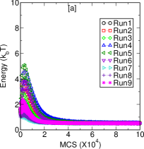
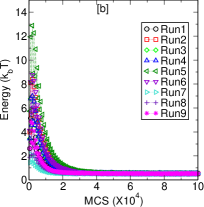
We monitor the potential energy as the chain relaxes. The value of energy relaxes to the same value at the end of $10^{5}$ iterations from the $9$ different runs, see Figure 1. It gives us confidence that the chain conformations are not stuck at metastable energy minima. From this initial state, we evolve each of the $9$ different chain conformations in independent simulation runs over the next $12\times 10^{6}$ iterations and collect data to calculate and compare structural quantities. We carry out this comparison of statistical data from $9$ independent runs for each set of CLs, viz., chains with (a) $47$ (b) $159$ CLs.

In addition, we also carry out similar calculations starting from $9$ independent initial configurations for each of the $10$ distinct sets of the randomly chosen position of CLs (monomers which are cross-linked together are chosen randomly from the list of monomers). The effective number of CLs for RC-1 and RC-2 correspond to the number of CLs in BC-1 and BC-2. In BC-1 and BC-2 set of CLs, there are some CLs which are not independent. For example, monomer number $16$ and $17$ are cross-linked to monomer $2515$ and $2516$, respectively. One cannot consider them as distinct CLs. The list of cross-linked monomers is given in Table-1 of Supplementary section TABLE $I$. Hence there are fewer effective CLs than the number of CLs in BC-1 and BC-2. Thus we compare the results of our simulation from bio-CLs (BC-1 and BC-2) with an equal number of effective random CLs. In each of these random set of CLs, we have the same number of effective CLs as the ones obtained from biological data, which is less than the corresponding number of CLs in BC-1 and BC-2. Hence the list of randomly positioned CLs have just (a) $27$ effective number of CLs (we refer these as RC-1) and (b) $82$ effective CLs (referred as RC-2), corresponding to $47$ CLs in BC-1 and $159$ CLs in BC-2. We can now compare structural data obtained from polymer simulations using BC-1 and RC-1 on the one hand, and BC-2 and RC-2 on the other.

III Results

Now we discuss the statistical quantities which we use to investigate the structure and conformation of the ring polymer. We aim to check if statistical quantities from $9$ different runs with the same set of CLs give similar results to infer that the polymer has similar shape and conformation across runs. We further compare data from $10$ different RC-1 and RC-2 CL sets with data from E.Coli CL set BC-1 and BC-2, though in this manuscript we show data primarily from one representative RC set.

The first quantity we want to estimate is the size and extent of the polymer with CLs. To that end, we calculate the moment of inertia tensor ${\mathbf{I}}$ with respect to the center of mass (CM) of the polymer coil and diagonalize the matrix to get its principal moments for each microstate. We then calculate the average principal moments $I_{1},I_{2},I_{3}$. where $I_{1}$ is the largest eigenvalue and $I_{3}$ the smallest.

Figure 2: (a) The value of $I_{1}/I_{3}$, the ratio of the largest and lowest eigenvalues of the diagonalized moment of inertia matrix for distinct random CL sets (no. of CLs for each RC-set is equal to that for RC-1 and RC-2, respectively). For each random CL-set index, the plot shows the average and s.d. of $I_{1}/I_{3}$ over $9$ independent initial conditions; the s.d. is smaller than the size of the symbol. (b) The value of $I_{1}/I_{3}$ versus run index for runs starting from $9$ independent initial conditions for biologically determined CLs: BC-1 and BC-2. (c) The plot of Radius of gyration $R_{g}=\sqrt{(I_{1}+I_{2}+I_{3})/3M)}$) versus the random CL-set index. (d) Plot of $R_{g}$ and run index from 9 independent initial conditions for biologically determined CLs: BC-1 and BC-2.

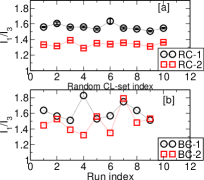
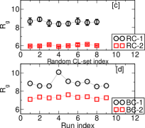
In Fig 2(a) we show the values of $(I_{1}/I_{3})$ for distinct random CL-sets but having the same number of CLs as RC-1 and RC-2. For each random CL-set, the average is taken over $9$ independent initial configurations. In subplot (b) we show $I_{1}/I_{3}$ for Biologically determined CLs: BC-1, BC-2 for 9 independent initial conditions. In plot (c) $R_{g}=\sqrt{(I_{1}+I_{2}+I_{3})/3M}$ for different random CL sets having same number of CLs as RC-1 and RC-2 is shown and in subplot (d) we show $R_{g}$ for $9$ independent initial conditions for BC-1 and BC-2 respectively. Here $M$ is the sum of masses of the individual monomers $M=\sum m_{i}$, $m_{i}=1$ is the mass of each monomer. The value of $I_{1}/I_{3}$ is the ratio of major and minor axes and gives a measure of shape asymmetry of the coil. Comparing the value of $I_{1}/I_{3}$ in 2(a), (b) we see that $I_{1}/I_{3}$ has a lower value for all ten RC-2 sets compared to BC-2 set. A plausible explanation for this difference is given later in this paragraph and confirmed by the end of this paper. Subplots Fig 2 (b) and (d) show the values of $R_{g}$ obtained from randomly determined CLs and Biologically determined CLs. The calculated value of $R_{g}$ for ring polymer without CLs and the average value is $\approx 12$. The value of $R_{g}$ decreases as we increase the number of CLs from BC-1/RC-1 set to BC-2/RC-2 sets; this decrease in the value with increase in the number of effective constraints is expected. But interestingly, the change in the value of $R_{g}$ as we go from BC-1 to BC-2 is distinctly less than the decrease in $R_{g}$ as we go from RC-1 to RC-2. We interpret the difference between the two cases as follows: the effective CLs in BC-1 are already at critical positions along the contour which give partial organization in the DNA. On increasing the number of CLs (BC-2), the organization of the molecule improves along the already established framework. On the other hand, an increase in the number of random CLs leads to an overall shrinkage in the size of the coil and not necessarily to accentuate a preferred set of conformations. The lower values of $I_{1}/I_{3}$ for all 10 sets of RC-2 compared to that in BC-2 also point towards such an understanding. This idea will get further substantiated in the rest of the paper.

Figure 3: The monomer number density of $n_{M}(r)$ is plotted versus $r$, where $r$ is the distance of the position of the monomers from the center of mass of the DNA-polymer coil. Plot (a) is for BC-1, RC-1, whereas plot (b) is for BC-2,RC-2. $n_{M}(r)$ is averaged over $9$ independent initial conditions and error bar shows the standard deviation from the average.

Figure 4: The normalized CL number density of $n_{CL}^{*}(r)$ is plotted versus $r$, where $r$ is the distance of the position of the CLs from the center of mass of the DNA-polymer coil. Subplot (a) is for BC-1 and RC-1, whereas subplot (b) is for BC-2 and RC-2. The number of CLs in each case is further normalized by the total number of CLs in each case. Further $n_{CL}^{*}(r)$ is averaged over 9 independent runs starting from initial conditions and error bar shows the standard deviation from the average.

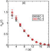
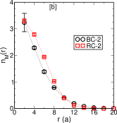
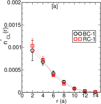
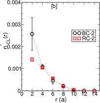
To get some idea of how the monomers of the polymer are distributed in space. And if there is any difference in the radial arrangement of bio-CLs and random CLs, we investigate the radial distribution of monomer number densities and the normalized CL number density with the distance $r$ from the center of mass (CM) of the polymer coil. The quantities $n_{M}(r)$ and $n_{CL}(r)$ are calculated by calculating the average number of monomers and CLs in radial shells of width $2a$ from the CM of the coil, divided by the volume of each shell. The CL-density is further normalized by the total number of CLs for the particular case under consideration to obtain $n_{CL}^{*}(r)$. Data for $n_{M}(r)$ and $n_{CL}^{*}(r)$ from $9$ independent runs are plotted for each of set of CLs: BC-1, BC-2, and one set of RC-1, RC-2 in Figs.3 and 4, respectively. Small standard deviation from average for monomer number densities and the normalized CL number density is an indication that the arrangement of monomers and CLs have relaxed to similar distributions and is independent of starting configuration of monomers.

Comparing subplots (a),(b) of Figs. 3 and 4 for BC-1 and BC-2, establishes that coils with a higher number of CLs lead to more number density of monomers and CLs at the center of the coil. As the coil gets into a more compact coil structure with increased number of CLs in set RC-2 as compared to RC-1, we again see an increase in the number density of monomers, CLs (suitably normalized) at the center. Comparing data for BC-1 and RC-1, respectively from Figs. 3 and 4, we observe that the distribution of monomers and CLs are similar at different $r$ for the 2 cases. In contrast, the normalized density of CLs at the central region is more for BC-2 compared to that for RC-2. Moreover, monomer density $n_{M}(r)$ for BC-2 is lower than that for RC-2 at the center of the coil, whereas there are more monomers present at the periphery (for $r>12s$) for BC-2 as compared to RC-2. Since the number of monomers in each shell is divided by the volume of the shell, the difference in the number of monomer at the periphery is just discernable from the number density $n_{M}(r)$ plots. Lastly, the number density of monomers/CLs drops down significantly beyond a distance of $8a$ from the coil’s center. Other nine sets of randomly chosen CLs also in tune with the above observations (data not shown).

Figure 5: Subplots (a), (b) and (c) (on left column) show the probabilities of individual CLs to be found in the inner, middle and outer region for CL-set BC-2. The x-axis is an index for CLs. The average is taken over 9 independent runs starting from different initial conditions, and standard deviation from the average is shown as an error bar. Small error bars indicate that the probability of finding CL $i$ is the same across different runs. Data (d), (e), (f) on the right column is for the set of random CLs RC-2. The set of 159 CLs for E. Coli are referred to as BC-2. Dataset with fewer number of E. Coli and random CLs (referred as BC-1 and RC-1, respectively) are shown in Supplementary Section Fig.16.

Figure 6: Subplots (a), (b) and (c) (in the left column) shows the probabilities of the center of mass (CM) of $80$ DNA-polymer segments to be found in the inner, middle and outer region of E. Coli DNA coil. The x-axis is segment index. In each case average values of $P_{inner},P_{middle}$ and $P_{outer}$ are taken over 9 runs starting from independent initial conditions, deviation from the average is shown as error bars. Small error bars indicate that the probability of finding CM of segment $i$ in a particular region is nearly the same across different runs. Data on subplots (d), (e), (f) is for random choice of cross-link position (set RC-2) with $82$ CLs in a chain with 4642 monomers. Each segment has 58 monomers. The dataset with fewer CLs (referred as BC-1 and RC-1, respectively) are shown in Supplementary Section Fig.17.

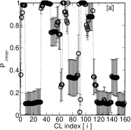
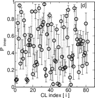
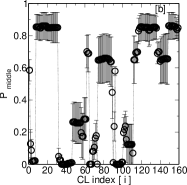
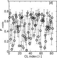
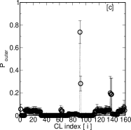
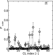
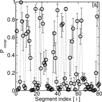
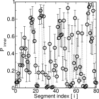
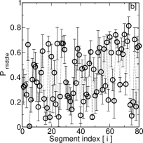
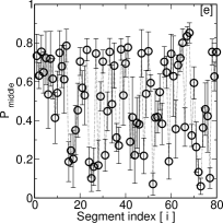
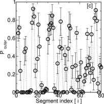
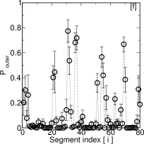
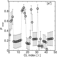
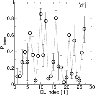
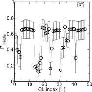
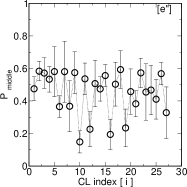
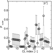
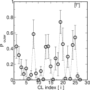
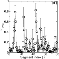
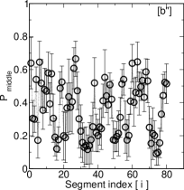
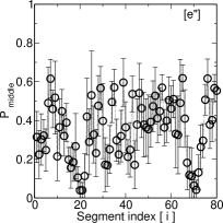
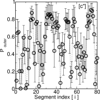
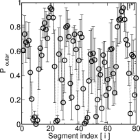
To gain some more insight about the global structural organization of the DNA-coil, the simplest question to ask is whether a particular CL is always found near the center of the coil or near the periphery of the coil. To this end, we compute the probability of each of the CLs to be found in the inner,middle, and outer regions of the DNA-coil. We use the cutoff radii $R_{inner}=5a$, $R_{middle}=9a$ (chosen from the knowledge of the value of $R_{g}\approx 8a$) and calculate the probability $P_{inner},P_{middle},P_{outer}$ of finding the $i-$th CL within distance $r<R_{inner}$ (inner region), $R_{inner}<r<R_{middle}$ (middle region) and $r>R_{middle}$ (outer region), respectively, from the coil’s center of mass. If the values of $P_{inner},P_{middle},P_{outer}$ for each CL has small deviation from the average value in each of the $9$ independent runs, it would indicate that the presence of CLs leads to similar organization of the DNA across independent runs. Also, we compare the probability distribution of CLs for runs with bio-CLs and random-CLs to investigate if bio-CLs lead to organization distinct from that obtained with random-CLs.

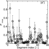
We carry out the same exercise for different segments of the polymer chain. The E. Coli chain with $4642$ monomers is divided into $80$ segments with $58$ monomers in each of segment and the segments are labeled from $i=1,2...N_{s}$ as we move along the contour. We can then calculate the location of the CMs of each segment, and find out the probability of finding the CMs in the central, middle and outer region. The segments in a random-walk polymer model (without CLs) can take any conformation, and there is no reason to believe that certain segments will preferably be found in the inner or outer regions of the coil. If the segments were completely delocalized, we would expect the polymer in different microstates to contribute to all the $P_{inner},P_{middle},P_{outer}$ quantities for each segment. The question is to what extent will this basic behavior of polymer coils get modified by the presence of bio-CLs and random-CLs?

Probability data about the location of CLs and segments for BC-2 and RC-2 is given in 5 and 6, respectively. Data for BC-1 and RC-1 is given in the Supplementary data section Fig.16, 17. Furthermore, from Figs 5 and 6(a),(b) and (c) we see that some CLs (e.g. the CL with index $60$) has the nearly equal probability of being in the inner or middle region of the coil, but very low probability to be found in the outer region. For BC-2, most CLs are found in the inner and middle regions of the coil whereas for RC-2 CL set there are some CLs at the periphery; refer Fig.5. On the other hand, from Fig.6 we see a larger number of segments have a finite probability to be in the outer regions for BC-2 as compared to data for RC-2. The data consistently shows that the position of CL, as well as segments are localized in space across different runs.

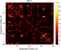
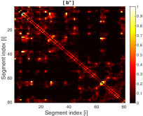
Having established that the CLs and segments of DNA-polymer coil have some degree of radial organization, we try to extract more detailed structural information about the position of segments relative to each other within the coil. We calculate the probability of each CL (alternatively, each segment) to be in proximity to other CLs (alternatively, other segments). If there are no particular well-defined relative positions of CLs/segments within the chain-coil, there is no reason to expect CM of some segments (or independent CLs) to be found spatially close to each other with high probability, especially when the segments/CLs are separated along the chain contour. We define two CLs/segment’s CM to be close to each other if the distance $r$ between the CLs/segment-CMs is $<5a$, which is just more than $0.5R_{g}$. We emphasize that we have cross-linked monomers, these constraints are at the monomer ($1000$ BP) length scale, whereas we are investigating the organization of polymer segments at a much larger length-scale. The position of CLs, position of CM of segments are just 2 different markers of different sections of the chain and we use relative position of both to identify spatial correlations between different sections of the chain.

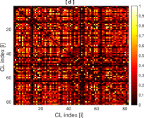
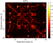
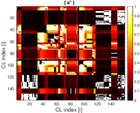
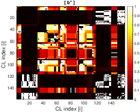
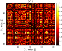
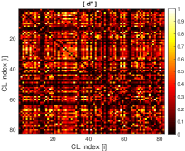
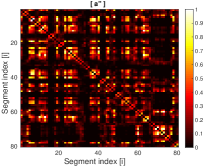
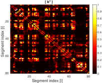
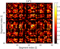
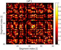
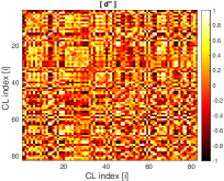
In Fig. 7 we show colormaps showing the average probability $p(i,j)$ of finding each pair CLs $i,j$ at distances of $<5a$ for BC-2, RC-2 for two independent runs. As the Monte Carlo simulation evolves, at each microstate if the distance $d$ between a pair of CLs is such that $d<5a$, a counter $c(i,j)$ for pair $i,j$ is incremented. The probability $p(i,j)$ at the end of the MC-run is the value of $p(i,j)=c(i,j)/N_{micro}$, where $N_{micro}$ is the number of microstates over which data is calculated for calculation. The x-axis and the y-axis represent CL indices $i,j$, and the colored pixel indicates the value of $p(i,j)$. The top two colormaps of Fig.7) represent data obtained for BC-2, and the bottom two colormaps Fig.7 show corresponding data from two independent runs with RC-2 set of CLs. A pair of CLs which are near each other along the contour of the chain will have the distance $d<5a$ between them by default, and will show up as high probabilities in the colormap. We set these $p(i,j)=0$ in the calculation if the monomers constituting pair of nearby CLs are separated by less than $6$ monomers along the contour. We do this because we want to see only non-trivial correlations between different CLs. Following Fig. 7, the colormaps show probability of finding a pair of segment-CMs within distance of $5a$ for BC-1/RC-1 and BC-2/RC-2 is shown in Figs.8 and 9, respectively. Note that these probability colormaps give much more detailed information than a pair correlation function $g(r)$, which would just give the average distance between CLs or segment-CMs.

Data showing probabilities $p(i,j)$ to find segments CM within a distance of $5a$ is shown in Figs.8 and 9 for BC-1,RC-1 and BC-2,RC-2, respectively. We arrive at some conclusions by comparing different pairs of probability-colormaps in Figs. 7,8 and 9. Firstly, comparing colormaps for data from different initial conditions, e.g. compare the top two colormaps in each of the figures which are for BC-1/BC-2 (or equivalently compare the bottom two colormaps which are for RC-1/RC-2), shows bright and dark patches at equivalent positions in the map. Thus the same set of CLs and segments are spatially near each other in both the runs, i.e. the polymer organization is similar in both the runs. Additional colormaps from two more independent runs for each set of CLs are also given in the Supplementary section for further comparison. The reference to relevant colormaps in the Supplementary section is given in the figure caption of each figure, and these further reiterates our conclusion that the structural organization of DNA-polymer is similar across different runs for the same set of CLs. Thus we find further evidence of our hypothesis that the set of CLs decides the large scale structure of the polymer.

Figure 7: Colormaps to represent probability $p(i,j)$ to find CLs $i$ spatially close CLs $j$. The top 2 figures are data from 2 independent runs with BC-2 with 159 CLs ($i,j=1...159$) and the bottom two subplots are from 2 independent runs with RC-2 with $i,j=1,....82$. More colormaps from independent runs are given in Supplem. Section: Fig.19.

Figure 8: Colormaps to represent probability $p(i,j)$ to find CM of segment $i$ spatially close to CMs of other chain segments $j$. There are $80$ segments in the E. Coli polymer with $58$ monomers per segment. The top 2 figures are runs with BC-1 and the bottom two for RC-1. More colormaps from independent runs are given in Supplem. Section: Fig.18.

Figure 9: Colormaps to represent probability $p(i,j)$ to find CM of segment $i$ spatially close to CMs of other chain segments $j$. There are $80$ segments in the E. Coli polymer with $58$ monomers per segment. The top 2 figures are runs with BC-2 and the bottom two subplots RC-2. More colormaps from independent runs are given in Supplem. Section: Fig.20.

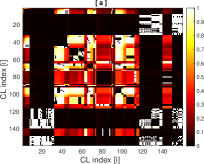
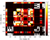
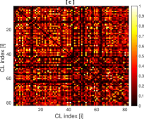
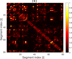
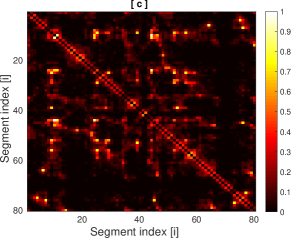
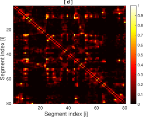
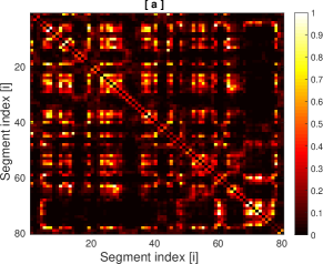
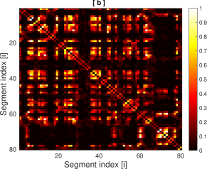
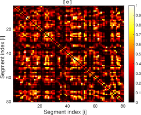
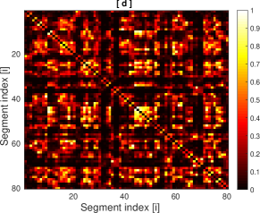
Secondly, the number of the bright pixels are much more in colormaps obtained using CL sets BC-2 and RC-2 (Figs.9) as compared to colormaps for BC-1 (Fig. 8). It is not surprising as more constraints due to the presence of higher number of CLs lead to relatively more compact well-defined structure and a large number of CLs (or segments) near one another. With the few bright patches for BC-1, RC-1 CL set with $27$ effective CLs, one cannot clearly define the mesoscale conformation of the whole chain, though there are indications of the emergence of structure. However, a set of $82$ effective CLs for BC-2, RC-2 might be enough to deduce and define the large-scale organization of DNA-polymer as we now know which segments are neighbors of a particular segment.

Thirdly, comparison of colormaps for BC-2 and RC-2, especially in Figs. 9 show a different nature of the organization of the DNA polymer. For BC-2 adjacent segments show higher propensity to be together, which can be deduced by observing that there are clusters of adjacent bright pixels. Comparatively, bright pixels are scattered more randomly in the colormaps for RC-2. From the colormaps, we can clearly, observe that there is a difference in the nature of patterns for BC-2 and RC-2.

Figure 10: Subplot (a) shows number of pixels $f(i)$ with probability $p(i,j)>0.05$ for a particular segment $i$ in the Fig. 9, normalized by the total number of segments versus the segment index. Subplot (b) shows $<f>$ for $10$ distinct random CL sets, labelled $K=1..10$ and one biologically determined CL set. The error bars show the standard deviation in $f_{av}$ (see text) calculated for the $9$ independent runs for each CL-set. Eighty-two pairs of monomers have been chosen randomly and then cross-linked for each CL set.

Fourthly and importantly, the reasons for the formation of clusters of bright pixels seen in the top two colormaps of Figs. 7 (for CLs) is not the same as that of Fig.9 (for segment-CMs). To understand the bright patches of Fig. 7, we remind the reader that the CLs are often found adjacent to each other along the chain contour for BC-1 and BC-2. Suppose, CL-$i$, CL-$j$ and CL-$k$ are next to each other along the chain. Note that then $p(i,j)$, $p(i,k)$,$p(j,k)$ has been explicitly put to zero. But if CL-$m$, which is far from $i$ and $j$ along the contour, comes within a distance of $5a$ from CL-$i$, then CL-$m$ is also automatically close to CL-$j,k$ and three adjacent pixels will appear in the colormap, viz., $p(i,m)$, $p(j,m)$,$p(k,m)$. Thus, the bigger bright patches for BC-2 in Fig. 7 should not necessarily be interpreted as evidence for a more organized polymer. A similar arrangement of bright/dark pixels across runs is just evidence of similar organization across different runs.

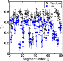
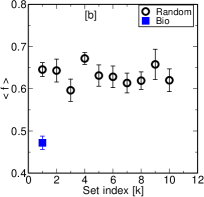
To quantify the differences in the colormaps of BC-2 and RC-2 in Fig. 9, we calculate the number of segments, $n_{seg}(i)$, which are near (i.e. within distance $d<5a$) to the CM of the $i$-th segment with probability $p(i,j)>0.05$. That is we count the number of non-black pixels in the colormaps of fig.9) for a particular segment with index $i$. Then we divide $n_{seg}(i)$ by the total number of segments to get $f(i)$ to get an estimate of the fraction of a total number of segments which approach segment $i$ with any finite probability. It is shown in the Fig.10 for RC-2 and BC-2. A cutoff of $0.05$ for the value of $p(i,j)$ is appropriate as anyways most of the colormap is black and deep red going upto yellow for very few pixels. From the figure, we observe that the value of $f(i)$ is relatively high for RC-2 set of CLs as compared to $f(i)$ for bio BC-2, this suggests for random CL-set many more segments can approach a particular segment for RC-2 compared to that for BC-2. We interpret this as a more spatially organized structure with BC-2 cross-links, as it has fewer but well-defined neighbors as can also be checked from the colormap of Fig.9. As an example, segments with indices 70-78 for BC-2 are only close to their adjacent segments (bright diagonal patch in the colormap) giving relatively very low value of $f(i)$ in Fig.10(a).

We have also obtained colormaps for the $10$ different sets of random CLs (data not shown), and for each CL-set we can calculate $f(i)$ for each segment index $i$. Moreover, we can calculate $f_{av}$, that is the average value of $f(i)$ summed over all the segment indices, i.e. $f_{av}=(\sum_{i}f(i))/80$. Furthermore, we can calculate the mean of $f_{av}$ over $9$ independent runs for each CL set, and thereby obtain $\langle f\rangle$. In Fig.10(b), we plot $\langle f\rangle$ versus the random CL-set index, each set has the same number of CLs as in RC-2. We compare this data with the $\langle f\rangle$ for the one set of biologically obtained CLs: BC-2. We clearly see that for each random CL-sets the quantity $\langle f\rangle$ has relatively higher value than $\langle$f$\rangle$ for BC-2. Observing the differences in colormaps for BC-2 and RC-2, we claim that the position of CLs along the chain for DNA are not completely random. An equivalent number of CLs in random positions also give an organized structure in that the colormaps from $9$ independent runs look similar, but the nature of organization is very different from the case where biological position of CLs are chosen.

To extract further insight into the structural organization of the DNA-polymer, we would next probe whether the segments are at geometrically fixed positions with respect to each other, of course accounting for thermal fluctuations. Thereby, we next calculate the angular correlations between CLs and equivalently between segment’s CMs.

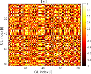
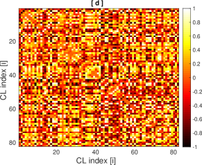
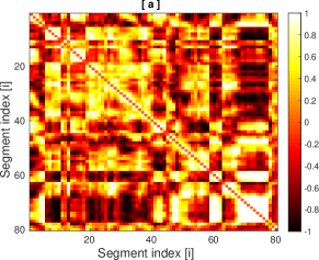
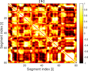
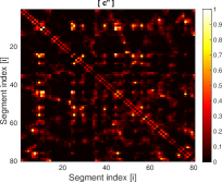
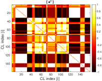
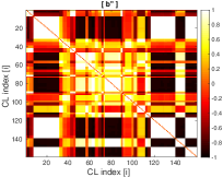
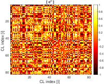
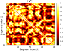
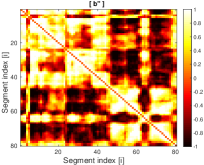
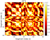
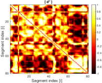
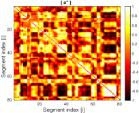
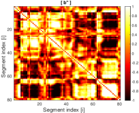
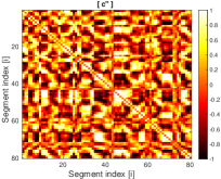
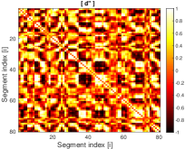
To that end, we calculate the dot product of the radial vectors from the CM of the polymer coil to the respective positions of a pair of CLs ($i,j$) and check if the value of $\cos(\theta_{ij})>0$ or $<0$, where $\theta_{ij}$ is the angle between the two vectors. If the value of $\cos(\theta_{ij})>0$, we can say that the two CLs are on the same side/hemisphere of the coil, and increment counter $c^{opp}(i,j)$ by $1$. If $\cos(\theta_{ij})<0$ we decrement $c^{opp}(i,j)$ by $1$. For all possible pairs of CLs, we calculate the average value of $\langle c^{opp}(i,j)\rangle$ suitably normalized by the number of snapshots used to calculate the average. The value of $\langle c^{opp}(i,j)\rangle\approx-1$ would indicate that the pair of CLs $i,j$ are always on two opposite hemispheres. A value of $\langle c^{opp}(i,j)\rangle\approx 1$ means that the two CLs remain on the same hemisphere. We should not interpret $\langle c^{opp}(i,j)\rangle\approx 0$ as we cannot claim that the average angle between the radial vectors is nearly a right angle. The reason is that if the CLs are closer to the center of the DNA-coil, small positional displacements could cause the quantity $c^{opp}(i,j)$ to fluctuate between $1$ and $-1$ and cause $\langle c^{opp}(i,j)\rangle$ to average out to zero. The $\langle c^{opp}(i,j)\rangle$ data for all pairs of CLs are given in Fig.11 for BC-2/RC-2 respectively, the corresponding data for relative angular positions for the segment’s CMs are given in Figs.12 & 13 for BC-1/RC-1 and BC-2/RC-2. As before, the top two colormaps in all the four figures are from two independent initial conditions with BC-1/BC-2 and the bottom two colormaps are for two independent runs with RC-1/RC-2.

In the colormaps of Figs. 11, 12 and 13 we see there are patches of bright and dark pixels, the size of patches are larger for BC-2 compared to RC-2. As mentioned before, if $\langle c^{opp}(i,j)\rangle=0$ which is represented by orange/deep yellow color in the colormap we cannot predict the angular positions of the CLs/segment’s CMs because of the reason explained above. We can clearly see that the colormaps from independent runs starting from different initial conditions look similar.

In figure 12, comparing segment-CM colormaps in (a),(b) (for BC-1) with (c),(d) (for RC-1) we do not find any difference in the nature of distribution of patches. But as the number of CLs increase as we go from BC-1 to BC-2 and RC-1 to RC-2 in Fig.13, we find differences in the pattern of colormaps on comparing (a),(b) with (c),(d) corresponding to BC-2 and RC-2 CL sets, respectively. In contrast, for color maps (a),(b) of Fig.13 we observe large patches of bright pixels as compared to the patches in (c),(d). Large patches of bright/dark pixels for BC-2 suggest adjacent segments along the chain contour are on the same/opposite hemispheres with respect to the CM of the coil. The small patches of bright and dark pixels in (c),(d) for RC-2 suggest more of random distribution of different segments. The polymer is organized in both BC-2 and RC-2 CL sets as colormaps from independent runs look similar, but the nature of the organization is different. The reasons for large bright patches in the colormaps for CL-angular positions as shown in Fig. 11 is not same as for the colormaps in Fig.13. The reasons for the difference has been explained previously for positional correlation colormaps.

Figure 11: Colormaps to investigate the angular location of different CLs with respect to each other. Subplots (a),(b) are for BC-2 and (c),(d) for RC-2 with different initial conditions, respectively. Refer Supplem. Section Fig.21 to compare with more colormaps from independent runs.

Figure 12: Colormaps to investigate the angular location of different DNA-polymer segments respect to each other. Subplots (a),(b) are for BC-1 and (c),(d) for RC-1 with different initial conditions, respectively. Refer Supplem. Section Fig.22 to compare with more colormaps from independent runs.

Figure 13: Colormaps to investigate the angular location of different DNA-polymer segments with respect to each other. Subplots (a),(b) are for BC-2 and (c),(d) for RC-2 with different initial conditions, respectively. Refer Supplem. Section Fig.23 to compare with more colormaps from independent runs.

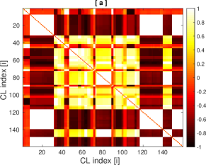
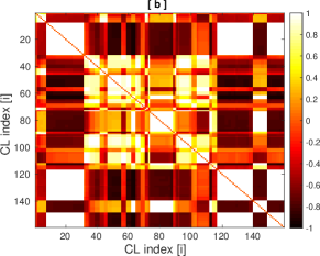
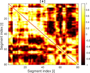
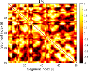
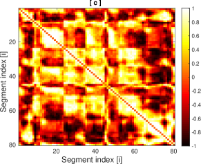
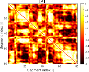
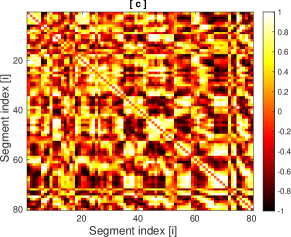
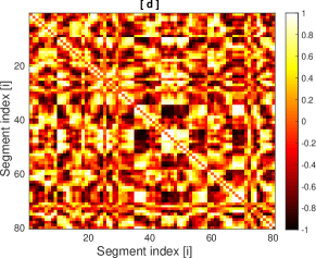
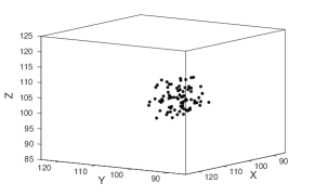
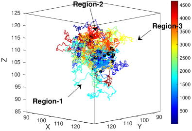
Finally, we show a representative snapshot of the DNA-polymer in Fig.14 (top). The polymer is colored from blue to red as we go from monomer index 1 to 4642 along the contour. This snapshot confirms what we have deduced from the previous figures of positional and angular correlations. Large sections of the chain are localized together in space. The snapshot confirms the kind of conformations expected from the colormaps of angular correlation shown in Fig.13(a) and (b). For example, the section marked Region-1 representing monomers around 1750 (segment index 30) is diametrically opposite Region-3 with monomer index 2990 (segment index 50). In Fig.13 (a) we see the pixel corresponding to segment indices (30,50) are black. The Region-2 represents monomer numbered around 4100, segment index 71. We can see the pixels corresponding to segment indices (30,71) is yellow whereas pixels for (50,71) is white. The bottom figure shows the CL distribution in space: only one of monomers out of the pair which constitutes a CL has been plotted.

Figure 14: Representative snapshot from our simulation of DNA-polymer with BC-2 is shown in the top figure. The color bar on the right shows the color which is used to represent the monomers numbered from $1$ to $4642$. The black circles show the positions of CLs. The bottom figure shows the position of CLs in space where we have removed the other monomers for better visualization. The coordinates are the same as used for the snapshot above. In bottom snapshot we see there are approximately 4 clusters of CLs in space for BC-2 while the CLs are uniformly distributed in space for RC-2 (refer Supplementary section Fig. 24).

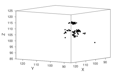
It is interesting to observe in Fig.14 (bottom) that the CLs are clumped together in space in about four aggregates. We believe that this helps in the mesoscale organization of the chain as multiple segments of the chain are pulled towards the coil’s center with multiple loops on the periphery of the coil. The peripheral loops can lead to relatively large fluctuations in the values of $I_{1}/I_{3}$ as seen in Fig.2. This is further validated by the Fig.6(c), where we see a large number of segments are to be found in the outer region with significant probabilities. Thus BC-2 set of cross-links leads to the reorganization of the CLs in space such that they form clusters in space with the possibility of polymer loops emanating from the CL-clusters in a rosette-like structure. We interpret that loops from a particular CL cluster would be neighbours of specific other polymer segments due to the nature of arrangement, as opposed to spatial proximity to many segments as seen for RC-2 in Fig.10 while comparing colormaps for BC-2 and RC-2.

Figure 15: Distribution of segment length between two adjacent CLs for BC-2 set and 4 different random CL sets corresponding to RC-2. The x-axis shows the length of the segments between two CLs and the y-axis shows the frequency density of segment’s length.

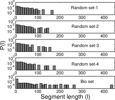
We also calculate the distribution of length of segments between two adjacent CLs in the bio and 4 representative random sets. It is given in the Fig.15. The distribution of lengths is a fixed quantity once one chooses a particular CL set as an input to the simulation. The number of segments of length $l$ between two adjacent CLs along the chain contour has been shown on x-axis (using a bin size $d\ell$ of 10 monomers) and the frequency density function (FDF) $P(l)$ is plotted on the y-axis, where $P(l)=N_{S}(l)/(N_{S}*d\ell)$. We denote the number of segments of length $\ell$ by $N_{S}(l)$ and $N_{S}$ is the total number of segments between CLs. Thus $N_{S}=82*2-1$ for RC-2 as each CL is constituted of a pair of monomers, and $l$ essentially is a count of the number of monomers between two CL-monomers along the contour. For the bio-CL, one particular monomer is attached with many other monomers (see supplementary material Table-1) hence there is a peak at segment length value $0$ to $10$. We also observe in the randomly chosen CL sets after segment length $\approx 150$ FDF is almost zero while in the biologically obtained CL set there are a few segments till segment length $\approx 400$. This shows in the biological CL set there are several longer segments which can form bigger loops as compared to CLs chosen in a random manner.

IV Discussion

The primary and new conclusions of our study is that if particular sets of monomers in a DNA-ring polymer are held together by suitable proteins (cross-links at specific points in our model polymer), it leads to an organization of the polymer coil. The number of effective CLs is 82 for a ring polymer of 4642 monomers, or approximately $2$% of the polymer chain. Moreover, the monomers which are cross-linked in the bacterial DNA are not randomly chosen from the length of the contour and lead to an organization of the ring polymer into a particular organization which is very different and distinct compared to what is obtained using an equal number of random cross-links. Of course, the DNA polymer undergoes local conformational fluctuations due to the thermal energy but overall the structure is maintained in a statistical sense. We can deduce the presence of distinctive mesoscale organization of DNA from the calculation of three quantities: (a) radial distribution of segments, (b) positional correlations between segments and (c) angular correlations between segments. Thus we have much more detailed information of organization of different segments than can be obtained from pair correlation function. We have used $159$ CLs for our simulation of DNA-polymer, but these should be considered as only $82$ effective CLs. A minimal number of CLs are required to be able to claim that there is a distinct organization of the DNA-polymer since we do not obtain a well-defined structure with $47$ bio-CLs (equivalently $27$ effective CLs). We can predict the 2-d arrangement of different segments relative to each other with the statistical quantities obtained. We find the clusters of CLs towards the center of the coil, these CLs are pulling different segments of the chain towards the center, and many loops on the periphery, which we interpret as the rosette-like structure. We have given a possible argument of how and why the structure with relatively well localized DNA-polymer segments is achieved in a polymer, but a full understanding and systematic methodology of the choice of CL-positions from the view of polymer physics can be developed only in future, when we will have access to the larger number of contact maps of many DNAs

V Supplementary Material

See supplementary material for the table of cross-linked monomers, colormaps of radial and angular correlations from additional runs and information of radial location of CLs and segments for BC-1 and RC-1.

VI Acknowledgments

We acknowledge the use of computational facilities provided by DBT Alliance, project numbers IA/I/12/1/500529,IA/I/11/2500290, to C. Assisi, S. Nadkarni, M.S. Madhusudhan. We also acknowledge the use of a cluster bought using DST-SERB grant no. EMR/2015/000018 to A. Chatterji. A. C. acknowledges funding support by DST Nanomission, India under the Thematic Unit Program (grant no.: SR/NM/TP-13/2016).

VII Appendix: Generation of contact frequency map

In the field of bioinformatics, a sequence database is a biological database which is a collection of computerized nucleic acid sequences. Paired-end sequencing allows researchers to sequence both ends of a DNA-fragment to generate high-quality, alignable sequence data. Paired-end sequencing facilitates detection of genomic reorganization and repetitive sequence elements.

In a paired end-sequencing run, the distance between the alignments of the two fragments is the length of the DNA fragment being sequenced. Aligners (software tools) use this information to better align reads when faced with a read that align to multiple regions such as those that may lie in a repeat region. To avoid this behavior, the reads are aligned in single end mode while keeping track of the pairs. We have employed the BWA Li and Durbin (2010) aligner to align reads as it has best sensitivity among short read aligners.

The aligned reads are then binned at the desired resolution (or the minimum distance between restriction sites). A 2D matrix with the required number of bins is initialized. A large fraction of the reads in a 3C library were from fragments that were not cross-linked and fall into the same bin or bins adjacent to each other. These read pairs were filtered out. The counter in the bin with the coordinates indicated by the alignment of each read in the pair is incremented for all the remaining reads. The filled matrix gives the total number of contacts between different parts of the genome and the resulting matrix is called the contact map.

To be able to compare between different runs, the contact map is normalized so that effect of varying number of sequenced reads is accounted for. Each sum of the number of contacts in each row and column in the matrix were normalized to 1. This provides a normalized contact map, which can now be used to elucidate the 3D structure of the genome and compare changes across different conditions.

Escherichia coli (E. coli) strain K12-MG1622 were obtained from German collection of microorganisms and cell cultures at Leibniz institute (DSMZ).

The aligned reads were then binned at the desired resolution (or the minimum distance between restriction sites). A 2D matrix with the required number of bins was initialized. A large fraction of the reads in a 3C library were from fragments that were not cross-linked and fall into the same bin or bins adjacent to each other. These read pairs were filtered out. The counter in the bin with the coordinates indicated by the alignment of each read in the pair is incremented for all the remaining reads. The filled matrix gives the total number of contacts between different parts of the genome and the resulting matrix is called the contact map. To be able to compare between different runs, the contact map were normalized so that effect of varying number of sequenced reads is accounted for. Each sum of the number of contacts in each row and column in the matrix were normalized to 1. This provides a normalized contact map, which can now be used to elucidate the 3D structure of the genome.

VIII List of cross-linked monomers in our simulations.

In the following table, we list the monomers which are cross-linked to model the constraints for the DNA of bacteria Caulobacter Crecentus. Note that for random cross links (CL) set-1 and set-2 (RC-1, RC-2) we have fewer number of CLs, as there are fewer effective CLs in the list of CLs.

In particular while counting the number of independent CLs, one should pay special attention to the points listed below. As a consequence, $47$ CLs of BC-1 should be counted as only $27$ independent CLs. Hence, we use just $26$ CLs in RC-1, when we compare organization of RC-1 and BC-1. Correspondingly, we have just $82$ CLs in RC-2, instead of $158$ in BC-2.

• The rows corresponding to independent cross-links of set BC-1 are marked by ^∗, one can observe that the next row of CLs are adjacent to the monomers marked just previously by ^∗. These cannot be counted as independent CLs.

• The rows marked by ⁺ is not a independent CL at all, monomers $-$ and $-$ are trivially close to each other by virtue of their position along the contour.

This table has been generated by analysis of raw data obtained from C. Cagliero et. al., Nucleic Acids Res, 41, 6058-6071 (2013).

Table 1: Table shows the list of pair of monomers which constitute the CLs for E.Coli, these CLs are used as an input to the simulation by constraining these monomers to be at a distance $a$ from each other. The first monomer with label $1$ and the last monomer labelled $4642$ are linked together because the DNA is a ring polymer.

-	BC-1		RC-1		BC-2		RC-2
Serial	Monomer	Monomer	Monomer	Monomer	Monomer	Monomer	Monomer	MOnomer
no.	index-1	index-2	index-1	index-2	Index-1	Index-2	Index-1	Index-2
1	1∗	4642	1	4642	1	4642	1	4642
2	16∗	2515	3739	4531	16	2515	3739	4531
3	17	2516	3011	1610	17	2516	3011	1610
4	20∗	1051	2582	4367	20	1051	2582	4367
5	224∗	2731	3370	1680	20	3584	3370	1680
6	225	2731	556	2622	21	1050	556	2622
7	226	2730	1676	1426	21	3584	1676	1426
8	226∗	3428	998	2741	224	2731	998	2741
9	227	2728	474	2233	224	3429	474	2233
10	227	2729	2522	533	224	4208	2522	533
11	228	2727	1967	2490	224	4209	1967	2490
12	228	2728	2536	616	225	2730	2536	616
13	229∗	2727	769	4614	225	2731	769	4614
14	271∗	4509	2	2023	226	2729	2	2023
15	272	4508	3494	2484	226	2730	3494	2484
16	275∗	1300	2534	1365	226	3427	2534	1365
17	280∗	1051	3053	2256	226	3428	3053	2256
18	291∗	1051	3779	2647	226	4038	3779	2647
19	316∗	393	4199	4452	226	4169	4199	4452
20	317∗	2172	2839	1309	227	2728	2839	1309
21	382∗	1469	1385	449	227	2729	1385	449
22	383	1469	4398	371	228	2727	4398	371
23	527∗	1529	522	1434	228	2728	522	1434
24	575∗	1301	3676	320	228	3946	3676	320
25	609∗	2515	178	4317	229	2727	178	4317
26	730∗	3763	3220	515	229	3424	3220	515
27	731	3764	527	2992	229	3947	527	2992
28	732	3765	-	-	229	3948	2391	1402
29	733+	735	-	-	229	4172	284	4086
30	733∗	3766	-	-	229	4213	4311	2243
31	1301∗	3132	-	-	229	4214	283	1687
32	1433∗	1635	-	-	271	4509	1599	2420
33	1434	1634	-	-	272	1471	4445	3365
34	1533∗	3626	-	-	272	4508	1523	739
35	1571∗	3667	-	-	274	1301	2721	113
36	1572	3668	-	-	275	1300	1371	4360
37	2728∗	3945	-	-	275	1301	4137	2593
38	2729	3945	-	-	275	3130	1026	2807
39	2730	3943	-	-	276	2291	3007	2767
40	3429∗	3942	-	-	276	3130	1576	1282
41	3471∗	4177	-	-	276	3367	3041	3010
42	3620∗	3763	-	-	280	292	2558	2709
43	3620	3764	-	-	280	1050	2156	3872
44	3621	3764	-	-	280	1051	945	4229
45	3622	3765	-	-	291	1051	4465	2873
46	3622	3766	-	-	291	2760	1943	4488
47	3623∗	3766	-	-	315	393	4286	881
48	-	-	-	-	316	391	3282	3882
49	-	-	-	-	316	392	3555	2445
50	-	-	-	-	316	393	1196	40
51	-	-	-	-	317	392	1997	3918
52	-	-	-	-	317	568	4178	1595
53	-	-	-	-	317	569	678	3768
54	-	-	-	-	317	1094	3519	164
55	-	-	-	-	317	1095	2979	4115
56	-	-	-	-	317	2172	2871	3747
57	-	-	-	-	382	1469	3930	4263
58	-	-	-	-	383	1468	2787	2654
59	-	-	-	-	383	1469	1101	831
60	-	-	-	-	393	567	2785	1485
61	-	-	-	-	393	1096	3477	1069
62	-	-	-	-	393	2171	2345	795
63	-	-	-	-	526	1529	4037	3848
64	-	-	-	-	527	1529	395	1040
65	-	-	-	-	527	1530	328	930
66	-	-	-	-	575	1301	1926	2551
67	-	-	-	-	576	3130	4440	1484
68	-	-	-	-	576	3367	3799	4456
69	-	-	-	-	581	1636	4129	837
70	-	-	-	-	581	1637	1500	1352
71	-	-	-	-	582	1636	3197	947
72	-	-	-	-	608	2515	263	3435
73	-	-	-	-	609	2515	2272	277
74	-	-	-	-	688	1301	4276	702
75	-	-	-	-	730	3763	3405	978
76	-	-	-	-	731	3763	388	3658
77	-	-	-	-	731	3764	2796	1022
78	-	-	-	-	732	3621	3411	1122
79	-	-	-	-	732	3764	861	2185
80	-	-	-	-	732	3765	3564	1606
81	-	-	-	-	733	735	1860	1447
82	-	-	-	-	733	3623	904	3577
83	-	-	-	-	733	3765	-	-
84	-	-	-	-	733	3766	-	-
85	-	-	-	-	734	3765	-	-
86	-	-	-	-	734	3766	-	-
87	-	-	-	-	738	1533	-	-
88	-	-	-	-	738	3626	-	-
89	-	-	-	-	782	2522	-	-
90	-	-	-	-	1051	3585	-	-
91	-	-	-	-	1208	1210	-	-
92	-	-	-	-	1269	1271	-	-
93	-	-	-	-	1301	1398	-	-
94	-	-	-	-	1301	2102	-	-
95	-	-	-	-	1301	2289	-	-
96	-	-	-	-	1301	3132	-	-
97	-	-	-	-	1301	3366	-	-
98	-	-	-	-	1301	3652	-	-
99	-	-	-	-	1397	2573	-	-
100	-	-	-	-	1397	3118	-	-
101	-	-	-	-	1433	1635	-	-
102	-	-	-	-	1434	1634	-	-
103	-	-	-	-	1435	1633	-	-
104	-	-	-	-	1469	2071	-	-
105	-	-	-	-	1470	2071	-	-
105	-	-	-	-	1470	2071	-	-
106	-	-	-	-	1470	2998	-	-
107	-	-	-	-	1470	3186	-	-
108	-	-	-	-	1470	4498	-	-
109	-	-	-	-	1470	4508	-	-
110	-	-	-	-	1470	4509	-	-
111	-	-	-	-	1471	4508	-	-
112	-	-	-	-	1533	3625	-	-
113	-	-	-	-	1533	3626	-	-
114	-	-	-	-	1571	3667	-	-
115	-	-	-	-	1572	3667	-	-
116	-	-	-	-	1572	3668	-	-
117	-	-	-	-	2726	4172	-	-
118	-	-	-	-	2727	4172	-	-
119	-	-	-	-	2728	3945	-	-
120	-	-	-	-	2728	4039	-	-
121	-	-	-	-	2728	4171	-	-
122	-	-	-	-	2729	3945	-	-
123	-	-	-	-	2729	4038	-	-
124	-	-	-	-	2730	3943	-	-
125	-	-	-	-	2730	4038	-	-
126	-	-	-	-	2731	3942	-	-
127	-	-	-	-	2731	4036	-	-
128	-	-	-	-	2732	3942	-	-
129	-	-	-	-	3424	4172	-	-
130	-	-	-	-	3426	3945	-	-
131	-	-	-	-	3426	4156	-	-
132	-	-	-	-	3427	3944	-	-
133	-	-	-	-	3427	4038	-	-
134	-	-	-	-	3428	3943	-	-
135	-	-	-	-	3428	3944	-	-
136	-	-	-	-	3429	3942	-	-
137	-	-	-	-	3471	4177	-	-
138	-	-	-	-	3472	4176	-	-
139	-	-	-	-	3472	4177	-	-
140	-	-	-	-	3619	3763	-	-
141	-	-	-	-	3620	3763	-	-
142	-	-	-	-	3620	3764	-	-
143	-	-	-	-	3621	3764	-	-
144	-	-	-	-	3621	3765	-	-
145	-	-	-	-	3622	3765	-	-
146	-	-	-	-	3622	3766	-	-
147	-	-	-	-	3623	3766	-	-
148	-	-	-	-	3623	3768	-	-
149	-	-	-	-	3942	4167	-	-
150	-	-	-	-	3942	4209	-	-
151	-	-	-	-	3943	4038	-	-
152	-	-	-	-	3944	4038	-	-
153	-	-	-	-	3944	4169	-	-
154	-	-	-	-	3944	4210	-	-
155	-	-	-	-	4036	4167	-	-
156	-	-	-	-	4036	4209	-	-
157	-	-	-	-	4037	4443	-	-
158	-	-	-	-	4041	4214	-	-
159	-	-	-	-	4172	4214	-	-

IX Radial location of CLs and segment’s CM of E.Coli.

In the main manuscript, we show the radial organization of different CLs and segment-CMs in Figs.6 and Fig.7, respectively for BC-2 and compare it with the DNA-polymer with CLs corresponding to RC-2, which has the same number of effective CLs as in BC-2. In the following, we give analogous plots with BC-1 and RC-1.

Figure 16: Data for bacteria E.Coli with no. of CLs = BC-1 : Subplots (a”), (b”) and (c”) show the probabilities of CLs to be found in the inner, middle and outer region of DNA globule. The x-axis is segment index, Each valuue of probability is the average over 9 independent initial conditions. Eroor bar shows the standard deviation. Subplots (d”), (e”), (f”) are for RC-1. Each segment has 58 monomers, the dna-polymer has around 80 segments.

Figure 17: Data for bacteria E.Coli with no. of CLs = BC-1 : Subplots (a”), (b”) and (c”) show the probabilities of center of mass of polymer segments to be found in the inner, middle and outer region of polymer globule. The x-axis is segment index. Each valuue of probability is the average over 9 independent initial conditions. Eroor bar shows the standard deviation. Subplots (d”), (e”), (f”) are for RC-1. Each segment has 58 monomers, the dna-polymer has around 80 segments.

X COLOR-MAPS for positional correlations

Figure 18: Colormaps show the probability of center of mass of the segments (i) (58 monomer each) to be found within a distance $5\sigma$ of other segment’s center of mass. The colormaps (a”), (b”) and (c”) and (d”) are from two additional independent runs for BC-1 and RC-1, respectively.

Figure 19: Colormaps show the probability to find CLs $i$ and CLs $j$ within a distance of $5\sigma$. The colormaps (a”), (b”) and (c”) and (d”) are from two additional independent runs for BC-2 and RC-2, respectively.

Figure 20: Colormaps show the probability of center of mass of the segments (i) (58 monomer each) to be found within a distance $5\sigma$ of other segment’s center of mass. The colormaps (a”), (b”) and (c”) and (d”) are from two additional independent runs for BC-2 and RC-2, respectively.

XI COLOR-MAPS for angular correlations

Figure 21: Colormaps show the angular positions of different CL with respect to each other. The colormaps (a”), (b”) and (c”) and (d”) are from two additional independent runs for BC-2 and RC-2, respectively.

Figure 22: Colormaps show the angular positions of center of mass of the different segments with respect to each other. The colormaps (a”), (b”) and (c”) and (d”) are from two additional independent runs for BC-1 and RC-1, respectively.

Figure 23: Colormaps show the angular positions of center of mass of the different segments with respect to each other. The colormaps (a”), (b”) and (c”) and (d”) are from two additional independent runs for BC-2 and RC-2, respectively.

XII Snapshot from simulation

Figure 24: Representative snaphots from our simulations of the positions of CLs for RC-2.

References

- Dekker et al. (2013) J. Dekker, M. A. Marti-Renom, and L. A. Mirny, Nat Rev Genet. 14, 390 (2013).
- Lieberman-Aiden et al. (2009) Lieberman-Aiden, N. L. van Berkum, L. Williams, M. Imakaev, I. A. T. Ragoczy, A. Telling, B. R. Lajoie, P. J. Sabo, M. O. Dorschner, B. B. R. Sandstrom, M. A. Bender, J. S. M. Groudine, A. Gnirke, L. A. Mirny, and J. D. E. S. Lander, Science 326, 289 (2009).
- Joyeux (2015) M. Joyeux, Journal of Physics: Condensed Matter 27, 383001 (2015).
- Dekker and Mirny (2016) J. Dekker and L. Mirny, Cell 164, 1110 (2016).
- Bickmore and van Steensel (2013) W. A. Bickmore and B. van Steensel, Cell 152, 1270 (2013.).
- Dixon et al. (2012) J. R. Dixon, S. Selvaraj, F. Yue, A. Kim, M. H. Y. Li, Y. Shen, J. S. Liu, and B. Ren, Nature 485, 376 (2012).
- Maxim V. Imakaev (2015) L. A. M. Maxim V. Imakaev, Geoffrey Fudenberg, FEBS Letters 589, 3031 (2015).
- Chaudhuri and Mulder (2012) D. Chaudhuri and B. M. Mulder, Phys. Rev. Lett. 108 (2012), 10.1103/PhysRevLett.108.268305.
- Jonathan D. Halverson and Grosberg (2014) K. K. Jonathan D. Halverson, Jan Smrek and A. Y. Grosberg, Reports on Progress in Physics 77 (2014.).
- Grosberg (2016) A. Y. Grosberg, Biophysical Journal 110, 2133–2135 (2016).
- Andreas Hofmann (2015) D. W. H. Andreas Hofmann, FEBS Letters 589, 2958 (2015).
- Ramakrishnan et al. (2015) N. Ramakrishnan, K. Gowrishankar, L. Kuttippurathu, P. B. S. Kumar, and M. Rao, “Active remodeling of chromatin and implications for in-vivo folding,” (2015), arXiv:1510.04157 .
- Fudenberg et al. (2016a) G. Fudenberg, M. Imakaev, C. Lu, A. Goloborodko, N. Abdennur, and L. A. Mirny, Cell Reports 15, 2038 (2016a).
- Rosa and Everaers (2008) A. Rosa and R. Everaers, PLOS Computational Biology 4:e1000153 (2008), 10.1371/journal.pcbi.1000153.
- Pombo and Nicodemi (2014) A. Pombo and M. Nicodemi, Current Opinion in Cell Biology, 28 (2014.).
- Chiariello et al. (2016a) A. M. Chiariello, C. Annunziatella, S. Bianco, A. Esposito, and M. Nicodemi, Nature Scientific Reports 6 (2016.a).
- Iyer and Arya (2012) B. V. S. Iyer and G. Arya, Phys. Rev. E 86 (2012), 10.1103/PhysRevE.86.011911.
- Le et al. (2013) T. B. K. Le, M. V. Imakaev, L. A. Mirny, and M. T. Laub., Science 342, 731 (2013).
- Cagliero et al. (2013) C. Cagliero, R. S. Grand, M. B. Jones, D. J. Jin, and J. M. O’Sullivan, Nucleic Acids Res. 41, 6058 (2013).
- Phillips-Cremins et al. (2013) J. E. Phillips-Cremins, M. E. Sauria, A. Sanyal, T. I. Gerasimova, B. R. Lajoie, J. S. Bell, C.-T. Ong, T. A. Hookway, C. Guo, Y. Sun, M. J. Bland, W. Wagstaff, S. Dalton, T. C. McDevitt, R. Sen, J. Dekker, J. Taylor, and V. G. Corces., Cell 153, 1281 (2013.).
- Imakaev et al. (2015) M. V. Imakaev, K. M. Tchourine, S. K. Nechaev, and L. A. Mirny, Soft Matter 11, 665 (2015).
- Mirny (2011) L. A. Mirny, Chromosome Res. 19, 37 (2011.).
- Vologodskii (2009) A. Vologodskii, Nucleic Acids Res. 37, 3125 (2009).
- Sachs et al. (1995) R. K. Sachs, G. van den Engh, B. Trask, H. Yokota, , and J. E. Hearst., PNAS U.S.A. 92, 2710 (1995.).
- Marenduzzo et al. (2006) D. Marenduzzo, C. Micheletti, and P. R. Cook, Biophysical Journal 90, 3712 (2006.).
- Bohn and Heermann (2010) M. Bohn and D. W. Heermann, PLoS ONE (2010), 10.1371/journal.pone.0012218, e12218 .
- Barbieri et al. (2012) M. Barbieri, M. Chotalia, J. Fraser, L.-M. Lavitas, J. Dostie, A. Pombo, and M. Nicodemi, PNAS U.S.A. 109, 16173 (2012).
- Fudenberg et al. (2016b) G. Fudenberg, M. Imakaev, C. Lu, A. Goloborodko, and N. Abdennur, Cell Reports 15, 2038 (2016b).
- Goloborodko et al. (2016) A. Goloborodko, J. F. Marko, and L. A. Mirny, Biophysical Journal 110, 2162 (2016).
- Rubinstein and Colby (2003) M. Rubinstein and R. H. Colby, Polymer physics (Oxford University Press, Oxford., 2003).
- Rob Phillips (2008) J. T. Rob Phillips, Jane Kondev, Physical Biology of the Cell (Garland Science., 2008).
- Maeshima et al. (2010) K. Maeshima, S. Hihara, and M. Eltsov, Current Opinion in Cell Biology 22, 291 (2010).
- Mateos-Langerak et al. (2009) J. Mateos-Langerak, M. Bohn, W. de Leeuw, O. Giromus, E. M. M. Manders, P. J. Verschure, M. H. G. Indemans, H. J. Gierman, D. W. Heermann, R. van Driel, and S. Goetze, PNAS U.S.A. 106, 3812 (2009).
- Chiariello et al. (2016b) A. M. Chiariello, C. Annunziatel, S. Bianco, A. Esposito, and M. Nicodemi, Scientific Reports 6 (2016b), 10.1038/srep29775.
- Gilbert et al. (2017) N. Gilbert, Marenduzzo, and Davide, Chromosome Research 25, 1 (2017).
- Fudenberg et al. (2016c) G. Fudenberg, M. Imakaev, C. Lu, A. Goloborodko, N. Abdennur, and L. A. Mirny, Cell Reports 15, 2038 (2016c).
- Alipour and Marko (2012) E. Alipour and J. F. Marko, Nucleic Acids Research 40 (2012), 10.1093/nar/gks925.
- Naumova et al. (2013) N. Naumova, M. Imakaev, G. Fudenberg, Y. Zhan, B. R. Lajoie, L. A. Mirny, and J. Dekker, Science 342, 948 (2013), http://science.sciencemag.org/content/342/6161/948.full.pdf .
- Rousseau et al. (2011) M. Rousseau, J. Fraser, M. A. Ferraiuolo, J. Dostie, and M. Blanchette, BMC Bioinformatics 12 (2011), 10.1186/1471-2105-12-414.
- Baù et al. (2011) D. Baù, A. Sanyal, B. R. Lajoie, E. Capriotti, M. Byron, J. B. Lawrence, J. Dekker, and M. A. Marti-Renom, Nature Structural & Molecular Biology 18, 107 (2011).
- Li and Durbin (2010) H. Li and R. Durbin, Bioinformatics, 26, 589 (2010.).
Supplementary Materials