An Adiabatic Invariant Approach to Transverse Instability:
Landau Dynamics of Soliton Filaments

Abstract

Consider a lower-dimensional solitonic structure embedded in a higher dimensional space, e.g., a 1D dark soliton embedded in 2D space, a ring dark soliton in 2D space, a spherical shell soliton in 3D space etc. By extending the Landau dynamics approach [Phys. Rev. Lett. 93, 240403 (2004)], we show that it is possible to capture the transverse dynamical modes (the “Kelvin modes”) of the undulation of this “soliton filament” within the higher dimensional space. These are the transverse stability/instability modes and are the ones potentially responsible for the breakup of the soliton into structures such as vortices, vortex rings etc. We present the theory and case examples in 2D and 3D, corroborating the results by numerical stability and dynamical computations.

Introduction. In numerous contexts, such as atomic physics stringari ; siambook , nonlinear optics kivshar , water waves water , and others dauxois , soliton dynamics is of crucial importance. It is then especially relevant, e.g., in external potentials confining Bose-Einstein condensates (BECs) or in refractive index landscapes in optics or, more recently, in gain/loss profiles of $\mathcal{PT}$-symmetric media yang , to be able to characterize the reduced degree-of-freedom evolution of soliton characteristics (center of mass, width, etc. kivmal ; malomed ).

While mathematical theories including those of nonlinear dispersive wave equations, such as the nonlinear Schrödinger (NLS) equation sulem ; ablowitz , are well developed in one-dimensional (1D) settings, solitons often emerge in (or experimental settings naturally feature) higher dimensional scenarios. Then, a question of paramount importance is that of the stability of e.g., 1D or quasi-1D (in the case of polar or spherical coordinates) solitonic “filaments” in the higher dimensional space in which they may be embedded. A classical example of an instability that may arise because of the transverse degrees of freedom, is the transverse modulational (or “snaking”) instability, first analyzed in Ref. kuzne for dark soliton stripes embedded in a 2D space. It has since then motivated many studies in optics and in atomic physics, exploiting as well as evading the instability, both theoretically smirnov ; us and experimentally brian .

In this work, our aim is to develop a theory that combines these two elements: considers the soliton motion, but explores it in a scenario where the solitonic structure is embedded in a higher dimensional space. Relevant examples include a 1D (rectilinear) soliton in a 2D domain, as is the case of Ref. kuzne , as well as two quasi-1D dark soliton structures: the ring dark soliton (RDS) and the dark spherical shell soliton (SSS), in 2D and 3D settings, respectively. RDSs were predicted kivyang (and observed rings ) in optics, and in BECs rings2 , while SSSs were studied in optics and BECs kivyang ; carr ; wenlong , and observed as transient structures in a BEC experiment hau . In earlier works, the so-called Landau dynamics approach (i.e., a semiclassical dynamics of the solitary wave as a quasi-particle relying on a local-density approximation) was developed for dark solitons konotop_pit ; konotop_pit2 and for RDSs korneev . Here, we adapt this approach towards accounting for the possibility of transverse instabilities, i.e., for transversely undulating soliton filaments. Employing this suitably modified technique, we analyze the (Kelvin) modes of transverse undulation, identify the modes of potential instability, and also offer a previously unknown class of partial differential equations (PDEs) unveiling the motion of the soliton filament within the higher dimensional space. The diversity of the above examples will serve to illustrate the broad applicability of this concept, well beyond the specific selections made herein.

Background and Transverse Instability of Planar Dark Solitons. Our starting point is the dimensionless (for relevant adimensionalizations in the BEC problem, see Refs. stringari ; siambook ) form of the 1D defocusing NLS equation:

$$iu_{t}=-\frac{1}{2}u_{xx}+|u|^{2}u+V(x)\,u.$$ (1)

In the absence of the external potential ($V\equiv 0$), and assuming a background density $\mu$, the dark soliton preserves the renormalized energy (see, e.g., the review djf ):

$$H_{\rm 1D}=\frac{1}{2}\int_{-\infty}^{\infty}\left[|u_{x}|^{2}+\left(|u|^{2}-\mu\right)^{2}\right]dx.$$ (2)

For the dark soliton solution of Eq. (1) (for $V=0$), with center $x_{0}$ and velocity $v=\dot{x}_{0}$, namely:

$$u=e^{-i\mu t}\left[\sqrt{\mu-v^{2}}\tanh\left(\sqrt{\mu-v^{2}}(x-x_{0})\right)+iv\right],~{}$$ (3)

the energy reads $H_{\rm 1D}=(4/3)(\mu-\dot{x}_{0}^{2})^{3/2}$. Then, according to the Landau dynamics approach konotop_pit ; konotop_pit2 this energy is treated as an adiabatic invariant in the presence of a slowly varying potential, i.e., the background density $\mu$ will be slowly varying according to $\mu\rightarrow\mu-V(x)$. Then, assuming the adiabatic invariance of

$$H_{\rm 1D}=\frac{4}{3}\left(\mu-V(x_{0})-\dot{x}_{0}^{2}\right)^{3/2}~{}\Rightarrow~{}\ddot{x}_{0}=-\frac{1}{2}V^{\prime}(x_{0}),$$ (4)

i.e., by its direct differentiation, one obtains the effective equation for the dark soliton center, in remarkable agreement with numerical results konotop_pit ; konotop_pit2 ; siambook ; djf .

Our proposal is to extend this notion of adiabatic invariants to the case of 1D stripes and quasi-1D RDSs embedded in 2D, as well as SSSs embedded in 3D. Our ultimate aim is not only to provide a fresh and broad/general perspective on the transverse instability, but also to describe the motion of the soliton filament in the higher dimensional space. It is known that in 2D as the undulation intensifies along the transverse direction, the soliton eventually decays into vortex-antivortex pairs smirnov ; dep . In 3D, the corresponding transverse instability gives rise to vortex rings and vortex lines siambook ; brian ; pindzola ; wenlong .

We specifically propose to consider the energy of a dark soliton stripe/filament again as an adiabatic invariant, whereby the 2D energy has an additional term:

$$H_{\rm 2D}=\frac{1}{2}\int_{-\infty}^{\infty}\left[|u_{x}|^{2}+|u_{y}|^{2}+\left(|u|^{2}-\mu\right)^{2}\right]dxdy.$$ (5)

Now, assuming an ansatz of the form of Eq. (3) with the center position not solely a function of $t$, but a function $x_{0}(y,t)$, we obtain an “effective energy” (an adiabatic invariant, again) of the form:

$$E=\frac{4}{3}\int_{-\infty}^{\infty}\left(1+\frac{{x_{0}}_{y}^{2}}{2}\right)\left(\mu-V(x_{0})-{x_{0}}_{t}^{2}\right)^{3/2}dy.$$ (6)

Based on this “effective Hamiltonian”, one can describe the transverse motion of the soliton filament. At the level of existence and stability of equilibria, one can use $x_{0}(y,t)=X_{0}(t)+\varepsilon X_{1}(t)\cos(ny)$, in order to (a) identify the leading order dynamical equation above [cf. second of Eqs. (4)], and (b) obtain the small amplitude —longitudinal, as well as transverse— excitations . Perhaps even more importantly, one can obtain from energy conservation the field-theoretic equation governing such a modulation. To simplify the exposition, for $V=0$, the relevant equation reads (see Supplement for details):

$$\left(1+\frac{{x_{0}}_{y}^{2}}{2}\right){x_{0}}_{tt}=\frac{1}{3}{x_{0}}_{yy}\left(\mu-{x_{0}}_{t}\right)+{x_{0}}_{t}{x_{0}}_{y}{x_{0}}_{ty}.$$ (7)

Importantly, at the linear level, this PDE is elliptic [${x_{0}}_{tt}+(\mu/3){x_{0}}_{yy}=0$] leading to the instability rate of Ref. kuzne . However, the key feature is that this novel, nonlinear PDE, Eq. (7), and its variant in the presence of the trap, can describe the nonlinear evolution of the soliton filament. When the latter leads to a jump discontinuity (a shock), then the filament breaks and develops the vortical patterns of principal interest herein.

A 2D Scenario: the Ring Dark Soliton (RDS). The RDS kivyang ; rings ; rings2 ; korneev is a quasi-1D solitonic structure (localized along the radial direction and extending as a filament along the azimuthal direction) embedded in 2D space; namely, a RDS is a circular dark soliton that closes into itself. The work of Ref. korneev utilized the argument of Ref. konotop_pit to a RDS of radius $R(t)$ and used the adiabatic invariant $E=2\pi R(\mu-\dot{R}^{2}-V(R))^{3/2}$ to obtain its purely radial equation of motion (see Supplement for details). Our Landau dynamics generalization considers this as a genuinely 2D filament whose radial position is $R(\theta,t)$, i.e., includes azimuthal “departures” from a perfect ring. Then, from the polar form of Eq. (5), the adiabatic invariant is generalized as:

$$E=\int_{0}^{2\pi}R\left(1+\frac{R_{\theta}^{2}}{2R^{2}}\right)\left(\mu-R_{t}^{2}-V(R)\right)^{3/2}d\theta.$$ (8)

From this equation, we can extract conditions for the existence of stationary RDS filaments of radius $R_{0}$ in a certain potential, and the stability (eigenfrequencies $\omega$) of small-amplitude excitations around it, using $R=R_{0}+\varepsilon\,e^{i(n\theta+\omega t)}$. These, respectively, read:

$$3R_{0}V^{\prime}(R_{0}) = 2(\mu-V(R_{0})),$$ (9)

$$\omega^{2} = \frac{V^{\prime}(R_{0})}{2R_{0}}\left[\frac{5}{3}-n^{2}+\frac{R_{0}V^{\prime\prime}(R_{0})}{V^{\prime}(R_{0})}\right].~{}~{}~{}$$ (10)

For the experimentally generic in BECs case of a parabolic potential, $V(R)=(1/2)\Omega^{2}R^{2}$ stringari ; siambook , we obtain

$$R_{0}^{2}=\frac{\mu}{2\,\Omega^{2}}\quad{\rm and}\quad\omega=\pm\left(\frac{1}{2}\left(\frac{8}{3}-n^{2}\right)\right)^{1/2}\Omega.$$ (11)

in very good agreement with asymptotic predictions of our numerical computations, as shown in Fig. 1 (see also for the equilibrium radius Fig. 14 in Ref. kaper ). It is important to highlight here that the above prediction enables a systematic and complete understanding of the modes of the Bogolyubov-de Gennes (BdG) linearization analysis in the asymptotic limit where this particle description is relevant, namely the Thomas-Fermi (TF) limit stringari ; siambook . This is due to the following fact: the spectrum of a nonlinear wave consists of the spectrum of the underlying “background” (the fundamental, equilibrium state on top of which the excitation exists) and the localized point spectrum associated with the excitation (the internal undulations of the solitary wave). In the BEC realm, the spectrum of the underlying ground state has been revealed in the fundamental work of Ref. stringari2 (see also Ref. dep2 ) and in 2D consists of the eigenfrequencies:

$$\omega=\pm\Omega(\ell+2k(1+\ell)+2k^{2})^{1/2},$$ (12)

for $k,\ell\geq 0$ (thin horizontal dashed lines in Fig. 1). Hence, the union of this set and of the eigenfrequencies of Eq. (11) (thin horizontal solid lines in Fig. 1) provides an unprecedented, all-encompassing theoretical prediction for the BdG spectrum of a RDS in the TF limit.

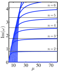
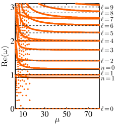
Figure 1: (Color online) Imaginary (left) and real (right) parts of the BdG excitation spectrum for the ring dark soliton (RDS). The former correspond to the instability modes, while the latter to the vibration modes. The thin horizontal solid lines in both panels correspond to undulation modes of the RDS in the Thomas-Fermi (large nonlinearity/large chemical potential $\mu$) limit, as predicted by Eq. (11). The thin horizontal dashed lines in the right panel correspond to the asymptotic predictions for the ground state spectrum for $k=0$ and $0\leq\ell\leq 9$ [cf. Eq. (12)]. To avoid clogging the relevant diagram, only the lowest modes of instability are shown.

Going one step beyond the equilibrium radius and the near-equilibrium vibrations, one can study the ring PDE evolution for $R(\theta,t)$. This can be obtained from energy conservation applied to Eq. (8). To illustrate this, we present two examples of dynamics comparing Eqs. (1) with the dynamics resulting from the energy functional (8), as shown in Fig. 2. Both cases correspond to non-ideal rings in the TF limit, for $\mu=24$ and $\Omega=1$. In one case, we have perturbed the rings with a combination of $n=0$, $n=1$, and $n=8$ modes with the initial condition $R(\theta)=2.8+0.1\cos(\theta)+3\times 10^{-7}\cos(8\theta)$ (top series of panels). In the second case, the ring is perturbed using a combination of $n=0$ and $n=2$ modes with the initial condition $R(\theta)=2.4+0.1\cos(2\theta)$ (bottom series of panels). The dynamics compare extremely well for the two PDEs until the rings significantly deform/break, illustrating that the PDE derived from the energy functional (8) is a valuable tool for understanding the evolution of ring soliton filaments. See Ref. movies for movies depicting the dynamics of these two examples and more definitively showcasing the comparison.

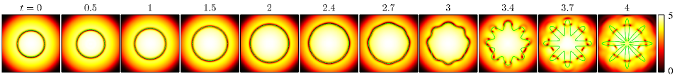
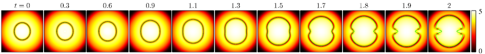
Figure 2: (Color online) Comparison of the full NLS dynamics (1) and the adiabatic invariant PDE obtained from Hamilton’s principle applied to Eq. (8) for a ring dark soliton (RDS) for $\mu=24$. Top series of panels: RDS with initial azimuthal position given by $R(\theta)=2.8+0.1\cos(\theta)+3\times 10^{-7}\cos(8\theta)$. Bottom series of panels: another RDS, but now with initial azimuthal position given by $R(\theta)=2.4+0.1\cos(2\theta)$. In both series of panels the top (bottom) subpanels depict the density (phase) of the solution on a $6\times 6$ square. The dynamics of the ensuing PDE is depicted by a solid green line. Note how the derived PDE closely follows the RDS dynamics before the break up of the latter into a series of vortex pairs.

A 3D Scenario: Dark Spherical Shell Soliton (SSS). Extending our considerations to a 3D case, we first study a 1D (rectilinear) dark soliton embedded (as a planar filament) in 3D space. For the soliton of Eq. (3) with center $x_{0}=x_{0}(y,z)$, the relevant energy functional reads:

$$E\!\!=\!\!\int\!\!\left(1+\frac{{x_{0}}_{y}^{2}}{2}+\frac{{x_{0}}_{z}^{2}}{2}\right)\!\left(\mu-V(x_{0})-{x_{0}}_{t}^{2}\right)^{3/2}\!dydz.~{}~{}$$ (13)

However, we do not focus on this simpler case (somewhat analogous to the 2D one), but rather consider the more intricate example of a quasi-1D dark SSS wenlong , localized along the radial direction with a center potentially undulating according to $R=R(\theta,\phi)$. Here, the adiabatic invariant of Landau dynamics subject to transverse undulations assumes the form:

$$E=\int R^{2}\left(1+\frac{R_{\theta}^{2}}{2R^{2}}+\frac{R_{\phi}^{2}}{2R^{2}\sin^{2}(\theta)}\right)$$

$$\times\left(\mu-R_{t}^{2}-V(R)\right)^{3/2}d\theta d\phi.$$ (14)

While the radial dynamics can be straightforwardly obtained wenlong , the calculation of the internal undulation modes is more technically involved, incorporating a decomposition of $R=R_{0}+\varepsilon R_{1}(\theta)R_{2}(t)\cos(n\phi)$ effectively into spherical harmonic modes. The shell’s equilibrium position $R_{0}$ satisfies:

$$3R_{0}V^{\prime}(R_{0})=4(\mu-V(R_{0})).$$ (15)

For the physically relevant (isotropic) parabolic potential $V(R)=(1/2)\Omega^{2}R^{2}$, this result leads to the equilibrium position $R_{0}=(4\mu/(5\Omega^{2}))^{1/2}$ in very good agreement with numerical results wenlong . The distilled final expression of the far more tedious eigenmodes calculation reads:

$$\frac{\omega^{2}}{\Omega^{2}}=\frac{7}{6}\frac{V^{\prime}}{R_{0}}+\frac{V^{\prime\prime}}{2}-\frac{V^{\prime}}{4R_{0}}\left(\frac{B}{A}+n^{2}\frac{C}{A}\right),$$ (16)

where $A=\int_{0}^{\pi}R_{1}^{2}\sin\theta d\theta$, $B=\int_{0}^{\pi}(R_{1}^{\prime})^{2}\sin\theta d\theta$ and $C=\int_{0}^{\pi}R_{1}^{2}\sin\theta d\theta$, while $V^{\prime}$ and $V^{\prime\prime}$ are evaluated at $R_{0}$. In this expression $R_{1}=P_{n}^{l}(\cos(\theta))$ corresponds to the associated Legendre polynomials. A closed form expression can be obtained, e.g., for $A=2(l+n)!/((2l+1)(l-n)!)$, yet generally these expressions amount to straightforward integral evaluations. In the particular case of the (spherical) parabolic trap, the expression becomes

$$\omega^{2}=\Omega^{2}\left(\frac{5}{3}-\frac{1}{4}\left(\frac{B}{A}+n^{2}\frac{C}{A}\right)\right).$$ (17)

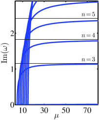
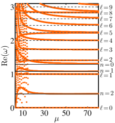
Figure 3: (Color online) The BdG excitation spectrum for the dark spherical shell soliton. The layout and meaning is the same as in the case of the ring dark soliton of Fig. 1. The thin horizontal solid lines correspond to the undulation modes in the TF limit, as predicted by Eq. (17), and the thin horizontal dashed lines to the asymptotic prediction for the ground state for $k=0$ and $0\leq\ell\leq 9$ [cf. Eq. (18)]. Once again, only the dominant instability modes are shown.

In this case too, combining the predictions of Eq. (17) with those for the vibration modes of the background (the ground state of the system), namely stringari2 ; dep2 :

$$\omega=\pm\Omega(\ell+3k+2k\ell+2k^{2})^{1/2},$$ (18)

with $k,\ell\geq 0$, one obtains the full linearization (BdG) spectrum of a dark SSS in the Thomas-Fermi limit. The relevant comparison illustrating once again the very good asymptotic agreement can be found in Fig. 3.

Conclusions $\&$ Future Work. In the present study, we provided a generalization of the theory of Landau dynamics as applied to solitary waves. We illustrated that this methodology can be extended to the formulation of soliton filaments and has the ability to provide a wealth of systematic results: (a) it can provide quantitative information about the equilibrium features of the solitonic filaments; (b) it can systematically characterize their stability in the form of undulation (Kelvin) modes, unveiling an unprecedented and complementary perspective on the transverse instability features; and (c) it can elucidate the dynamics proper of the solitonic filament, yielding insights on the potential amplification and eventual breakdown (i.e., formation of vortices and vortex rings) of the soliton filaments. Importantly, it should be underlined that our aim is not to manifest the advantages of this method over other methods (e.g., soliton perturbation theory kivmal or the variational approach malomed ) that treat solitary waves as quasi-particles. It is rather to highlight that some of these approaches (in fact, the variational approach can be similarly extended to address transverse instabilities and soliton filament motion) can be suitably “embedded” in higher dimensions and thus enable the detailed characterization of soliton filament motion.

This emerging theory of soliton filaments is promising in a broad range of directions. In addition to its usefulness for studying the modes of droplets and dynamics in other (e.g., magnetic hoefer ) systems, it can be used to obtain further insights on the dynamics of vortex and vortex-ring creation. From the point of view of the energy functionals and resulting PDEs for the solitonic filaments, the emergence of these other coherent structures is nothing but a collapse phenomenon. Hence, studying (possibly self-similar or asymptotically self-similar) collapse sulem ; galaktionov of the resulting PDEs is a particularly appealing future topic. Moreover, the technique is by no means constrained to dark solitons; for instance, as was discussed in Ref. JacksonMcCannAdams , using the energy of a vortex and a suitable azimuthal integration, one can obtain the energy of a vortex ring. If now the center of the vortex (in $R,Z$) varies as $R=R(\theta)$ and $Z=Z(\theta)$, then the undulations of a vortex ring (Kelvin modes) can be identified and compared with the corresponding BdG results horng ; bisset .

As an aside, we should mention here that the work of Ref. smirnov presents an alternative to the present method that may be especially powerful due to its intrinsic character. Considering the soliton filament as a curve if embedded in 2D (or as a surface if embedded in 3D), one can derive effective reduced PDEs for intrinsic quantities such as the curvature (or the torsion), as well as its coupling to the speed of the motion of the curve (or surface). This is a particularly appealing formulation to pursue in the near future.

Finally, it would be relevant to consider extending the adiabatic invariant approach to include the effects of dissipation. Such a generalization would need to involve a Hamiltonian formulation for PDEs similar to the Lagrangian formulation used in Ref. Panos_NCVA for $\mathcal{PT}$-symmetric sine-Gordon and $\phi^{4}$ models including gain and loss and in Ref. Julia_NCVA for NLS models including gain and loss, which in turn, were inspired by the work of Ref. Galley on classical, finite dimensional, mechanics of nonconservative systems; see also galley2 . Some of these directions are presently under consideration and will be reported in future works.

Acknowledgments. P.G.K. gratefully acknowledges support from the Alexander von Humboldt Foundation, the US-NSF under grants DMS-1312856, and PHY-1602994. W.W. acknowledges support from NSF-DMR-1151387. The work of W.W. is supported in part by the Office of the Director of National Intelligence (ODNI), Intelligence Advanced Research Projects Activity (IARPA), via MIT Lincoln Laboratory Air Force Contract No. FA8721-05-C-0002. The views and conclusions contained herein are those of the authors and should not be interpreted as necessarily representing the official policies or endorsements, either expressed or implied, of ODNI, IARPA, or the U.S. Government. The U.S. Government is authorized to reproduce and distribute reprints for Governmental purpose notwithstanding any copyright annotation thereon. R.C.G. gratefully acknowledges support from US-NSF under grants DMS-1309035 and PHY-1603058. We thank Texas A&M University for access to their Ada cluster. P.G.K. and D.J.F. gratefully acknowledge the Stavros Niarchos Foundation via the Greek Diaspora Fellowship Program.

APPENDIX

I Derivation of Equations for the Dark Soliton Stripe.

Firstly, we provide here a proof of the dynamics for a dark soliton stripe [Eq. (7) in the main text] starting from the corresponding adiabatic invariant Hamiltonian. The conservation of this Hamiltonian leads to

$$\frac{dE}{dt} = \frac{4}{3}\int_{-\infty}^{\infty}\frac{\partial}{\partial t}\left[\left(1+\frac{{x_{0}}_{y}^{2}}{2}\right)\left(\mu-V(x_{0})-{x_{0}}_{t}^{2}\right)^{3/2}\right]dy$$ (19)

$$= 0.$$

Using the notation

$$A \equiv \mu-V(x_{0})-{x_{0}}_{t}^{2},$$

$$B \equiv 1+\frac{{x_{0}}_{y}^{2}}{2},$$

the integrand $I$ of the above integral reads

$$I={x_{0}}_{y}{x_{0}}_{yt}A^{3/2}+\frac{3}{2}A^{1/2}B\left(-V^{\prime}(x_{0}){x_{0}}_{t}-2{x_{0}}_{t}{x_{0}}_{tt}\right).$$

Now, if we integrate by parts the first term in the integral, assuming boundary conditions such that surface terms disappear, we obtain

$$\int_{-\infty}^{\infty}{x_{0}}_{y}{x_{0}}_{yt}A^{3/2}dy=-\int_{-\infty}^{\infty}{x_{0}}_{t}\left({x_{0}}_{y}A^{3/2}\right)_{y}dy.$$

Now all the terms in the integral multiply ${x_{0}}_{t}$ and hence in order for the integral to vanish for arbitrary choices of $x_{0}$, the term multiplying ${x_{0}}_{t}$ should vanish. In fact, this is rather intuitive because the reverse process (i.e., multiplying the resulting equation by ${x_{0}}_{t}$ and integrating over $y$) leads naturally to the conservation law for the energy. This way, we obtain the final PDE for the filament’s dynamical evolution:

$${x_{0}}_{tt}B\!+\!\frac{1}{3}{x_{0}}_{yy}A\!=\!{x_{0}}_{y}{x_{0}}_{t}{x_{0}}_{yt}\!-\!\frac{1}{2}V^{\prime}(x_{0})\left(B\!-\!{x_{0}}_{y}^{2}\right).$$ (20)

Equation (20) has a number of meaningful limits:

• Near the linear limit, as indicated in the main text, it leads to

  $${x_{0}}_{tt}+\frac{\mu}{3}{x_{0}}_{yy}=0,$$ (21)

  yielding the proper linear growth rate of the transverse instability SSSkuzne .

• If $x_{0}=x_{0}(t)$ only, it recovers the celebrated result for the single dark soliton (obtained originally by Busch and Anglin SSSbusch and also by Konotop and Pitaevskii SSSkonotop_pit ),

• In the case where there is no potential, i.e., for $V(x_{0})=0$, it yields Eq. (7) in the main text, namely:

  $${x_{0}}_{tt}B+\frac{1}{3}{x_{0}}_{yy}(\mu-{x_{0}}_{t}^{2})={x_{0}}_{y}{x_{0}}_{t}{x_{0}}_{yt}.$$ (22)

II Derivation of Equations for the Ring Dark Soliton.

We proceed in a similar fashion for the derivation of the equation of motion in the case of the ring dark soliton. Using the notation

$$C \equiv \mu-V(R)-{R}_{t}^{2},$$

$$D \equiv 1+\frac{R_{\theta}^{2}}{2R^{2}},$$

we obtain that:

$$\frac{3}{4}\frac{dE}{dt} = \int_{0}^{2\pi}\left[R_{t}DC^{3/2}+\frac{R_{\theta}R_{\theta t}}{R}C^{3/2}-\frac{R_{\theta}^{2}}{R^{2}}R_{t}C^{3/2}\right.$$ (23)

$$+ \left.\frac{3}{2}RDC^{1/2}(-V^{\prime}(R)-2R_{tt})R_{t}\right]d\theta=0.$$

Following a similar pattern as the derivation in the previous section, we recognize that all other terms multiply $R_{t}$ except for the second one, for which we use integration by parts as follows:

$$\int_{0}^{2\pi}\frac{R_{\theta}R_{\theta t}}{R}C^{3/2}d\theta=-\int_{0}^{2\pi}R_{t}\frac{\partial}{\partial\theta}\left(\frac{R_{\theta}}{R}C^{3/2}\right)d\theta.$$

Here, the surface terms disappear due to the periodic boundary conditions in the angular variable. As a result, once again all terms multiply $R_{t}$ and hence this multiplicative prefactor of $R_{t}$ in the angular integral has to vanish for the integral to generically vanish. The resulting PDE for the ring evolution reads:

$$CD-\frac{R_{\theta\theta}}{R}C = -\frac{R_{\theta}}{R}\left(\frac{3}{2}V^{\prime}(R)R_{\theta}+3R_{t}R_{t\theta}\right)$$ (24)

$$+ RD\left(\frac{3}{2}V^{\prime}(R)+3R_{tt}\right)$$

Again a series of special limits are of particular value:

• For the homogeneous steady state (time- and angle-independent $\theta$) $R_{0}$, we obtain $\mu-V(R_{0})=\frac{3}{2}R_{0}V^{\prime}(R_{0})$, in line, e.g., with Ref. SSSkaper .

• In the case of angle-independent radial motion, we obtain

  $$R_{tt}=\frac{C}{3R}-\frac{1}{2}V^{\prime}(R),$$ (25)

  in agreement with Ref. SSSkorneev .

• Finally, assuming $R=R_{0}+\epsilon R_{1}(t)\cos(n\theta)$, we obtain to O$(\epsilon)$ the evolution for $R_{1}$ in the form:

  $${R_{1}}_{tt}=\frac{V^{\prime}(R_{0})}{3R_{0}}\left[-\frac{5}{2}+\frac{3}{2}n^{2}-\frac{3}{2}\frac{R_{0}V^{\prime\prime}(R_{0})}{V^{\prime}(R_{0})}\right]R_{1}.$$ (26)

  Assuming $R_{1}\sim e^{i\omega t}$, we obtain the modes of vibration

  $$\omega^{2}=\frac{V^{\prime}(R_{0})}{2R_{0}}\left[\frac{5}{3}-n^{2}+\frac{R_{0}V^{\prime\prime}(R_{0})}{V^{\prime}(R_{0})}\right]$$ (27)

  In the case of a parabolic trap, $V(r)=\frac{1}{2}\Omega^{2}r^{2}$, this leads to $\omega=\Omega((8/3-n^{2})/2)^{1/2}$. These constitute Eqs. (10) and (11) in the main text.

References

- (1) L. P. Pitaevskii and S. Stringari, Bose-Einstein Condensation, Oxford University Press (Oxford, 2003).
- (2) P. G. Kevrekidis, D. J. Frantzeskakis, and R. Carretero-González, The Defocusing Nonlinear Schrödinger Equation, SIAM (Philadelphia, 2015).
- (3) Yu. S. Kivshar and G. P. Agrawal, Optical solitons: from fibers to photonic crystals, Academic Press (San Diego, 2003).
- (4) M. J. Ablowitz, Nonlinear dispersive waves: Asymptotic analysis and solitons, Cambridge University Press (Cambridge, 2011).
- (5) T. Dauxois, M. Peyrard, Physics of Solitons, Cambridge University Press (Cambridge, 2006).
- (6) S. V. Suchkov, A. A. Sukhorukov, J. Huang, S. V. Dmitriev, C. Lee and Yu.S. Kivshar, Laser Photon. Rev. 10 177 (2016); V. V. Konotop, J. Yang, and D. A. Zezyulin, Rev. Mod. Phys. 88 035002 (2016).
- (7) Yu. S. Kivshar and B. A. Malomed, Rev. Mod. Phys. 61, 763 (1989).
- (8) B. A. Malomed, Progress in Optics 43, 71 (2002).
- (9) C. Sulem and P. L. Sulem, The Nonlinear Schrödinger Equation, Springer-Verlag (New York, 1999).
- (10) M. J. Ablowitz, B. Prinari, and A. D. Trubatch, Discrete and Continuous Nonlinear Schrödinger Systems, Cambridge University Press (Cambridge, 2004).
- (11) E. A. Kuznetsov and S. K. Turitsyn, Zh. Eksp. Teor. Fiz. 94, 119 (1988) [Sov. Phys. JETP 67, 1583 (1988)].
- (12) V. A. Mironov, A. I. Smirnov, and L .A. Smirnov, Zh. Eksp. Teor. Fiz. 139, 55 (2011) [Sov. Phys. JETP 112, 46 (2011)].
- (13) See, e.g., the discussion of: M. Ma, R. Carretero-González, P. G. Kevrekidis, D. J. Frantzeskakis, and B. A. Malomed, Phys. Rev. A 82, 023621 (2010) and references therein.
- (14) B. P. Anderson, P. C. Haljan, C. A. Regal, D. L. Feder, L. A. Collins, C. W. Clark, and E. A. Cornell, Phys. Rev. Lett. 86, 2926 (2001).
- (15) Yu. S. Kivshar and X. Yang, Phys. Rev. E 50, R40 (1994).
- (16) D. Neshev, A. Dreischuh, V. Kamenov, I. Stefanov, S. Dinev, W. Fliesser, and L. Windholz, Appl. Phys. B 64, 429 (1997); A. Dreischuh, D. Neshev, G. G. Paulus, F. Grasbon, and H. Walther, Phys. Rev. E 66, 066611 (2002).
- (17) G. Theocharis, D. J. Frantzeskakis, P. G. Kevrekidis, B. A. Malomed, and Yu. S. Kivshar, Phys. Rev. Lett. 90, 120403 (2003).
- (18) L. D. Carr and C. W. Clark, Phys. Rev. A 74, 043613 (2006).
- (19) W. Wang, P. G. Kevrekidis, R. Carretero-González, and D. J. Frantzeskakis, Phys. Rev. A 93, 023630 (2016).
- (20) N. S. Ginsberg, J. Brand, and L. V. Hau, Phys. Rev. Lett. 94, 040403 (2005).
- (21) V. V. Konotop and L. P. Pitaevskii, Phys. Rev. Lett. 93, 240403 (2004).
- (22) V. A. Brazhnyi, V. V. Konotop, and L. P. Pitaevskii, Phys. Rev. A 73, 053601 (2006).
- (23) A. M. Kamchatnov and S. V. Korneev, aPhys. Lett. A 374, 4625 (2010).
- (24) D. J. Frantzeskakis, J. Phys. A 43, 213001 (2010).
- (25) Yu. S. Kivshar and D. E. Pelinovsky, Phys. Rep. 331, 117 (2000).
- (26) D. L. Feder, M. S. Pindzola, L. A. Collins, B. I. Schneider, and C. W. Clark, Phys. Rev. A 62, 053606 (2000).
- (27) W. Wang, P.G. Kevrekidis, R. Carretero-González, D.J. Frantzeskakis, T.J. Kaper, and M. Ma Phys. Rev. A 92, 033611 (2015).
- (28) S. Stringari, Phys. Rev. Lett. 77, 2360 (1996).
- (29) P. G. Kevrekidis and D. E. Pelinovsky, Phys. Rev. A 81, 023627 (2010).
- (30) See http:nonlinear.sdsu.edu/carreter/AI.html for animations depicting the dynamics ensuing from the destabilization of the ring dark soliton for the two different initial conditions.
- (31) D. Xiao, V. Tiberkevich, Y. H. Liu, Y. W. Liu, S. M. Mohseni, S. Chung, M. Ahlberg, A. N. Slavin, J. Akerman, Yan Zhou, arXiv:1610.06650.
- (32) V. A. Galaktionov, E. L. Mitidieri, and S. I. Pohozaev, Blow-up for Higher-Order Parabolic, Hyperbolic, Dispersion and Schrödinger Equations, CRC Press (Boca Raton, 2015).
- (33) B. Jackson, J.F. McCann, and C. S. Adams, Phys. Rev. A 61, 013604 (1999)
- (34) T.-L Horng, S.-C. Gou, T.-C. Lin, Phys. Rev. A 74, 041603 (2006).
- (35) R. N. Bisset, Wenlong Wang, C. Ticknor, R. Carretero-González, D. J. Frantzeskakis, L. A. Collins, and P. G. Kevrekidis, Phys. Rev. A 92, 063611 (2015).
- (36) P. G. Kevrekidis, Phys. Rev. A 89 010102 (2014).
- (37) J. Rossi, R. Carretero-González, and P.G. Kevrekidis, arXiv:1508.07040 [nlin.PS]; J. Rossi, R. Carretero-González, P.G. Kevrekidis, and M. Haragus, J. Phys. A 49 455201 (2016).
- (38) C. R. Galley, Phys. Rev. Lett. 110, 174301 (2013).
- (39) C. R. Galley, D. Tsang, L.C. Stein, arXiv:1412.3082.

References

- (1) E. A. Kuznetsov and S. K. Turitsyn, Zh. Eksp. Teor. Fiz. 94, 119 (1988) [Sov. Phys. JETP 67, 1583 (1988)].
- (2) Th. Busch and J. R. Anglin Phys. Rev. Lett. 84, 2298 (2000).
- (3) V. V. Konotop and L. P. Pitaevskii, Phys. Rev. Lett. 93, 240403 (2004).
- (4) W. Wang, P.G. Kevrekidis, R. Carretero-González, D.J. Frantzeskakis, T.J. Kaper, and M. Ma Phys. Rev. A 92, 033611 (2015).
- (5) A. M. Kamchatnov and S. V. Korneev, Phys. Lett. A 374, 4625 (2010).