Topological deconfinement transition in QCD at finite isospin density

Abstract

The confinement-deconfinement transition is discussed from topological viewpoints. The topological change of the system is achieved by introducing the dimensionless imaginary chemical potential ($\theta$). Then, the non-trivial free-energy degeneracy becomes the signal of the deconfinement transition and it can be visualized by using the map of the thermodynamic quantities to the circle $S^{1}$ along $\theta$. To understand this “topological” deconfinement transition at finite real quark chemical potential ($\mu_{\mathrm{R}}$), we consider the isospin chemical potential ($\mu_{\mathrm{iso}}$) in the effective model of QCD. The phase diagram at finite $\mu_{\mathrm{iso}}$ is identical with that at finite $\mu_{\mathrm{R}}$ outside of the pion-condensed phase at least in the large-$N_{\mathrm{c}}$ limit via the well-known orbifold equivalence. In the present effective model, the topological deconfinement transition does not show a significant dependence on $\mu_{\mathrm{iso}}$ and then we can expect that this tendency also appears at small $\mu_{\mathrm{R}}$. Also, the chiral transition and the topological deconfinement transition seems to be weakly correlated. If we will access lattice QCD data for the temperature dependence of the quark number density at finite $\mu_{\mathrm{iso}}$ with $\theta=\pi/3$, our surmise can be judged.

1 Introduction

Understanding the confinement-deconfinement transition is one of the important subjects in the particle and nuclear physics. In the heavy quark mass limit, the Polyakov loop respecting the gauge invariant holonomy characterizes the deconfinement transition. In that case, the spontaneous $\mathbb{Z}_{3}$ symmetry breaking describes the deconfinement transition and the Polyakov-loop becomes the order parameter of the symmetry breaking. On the other hand, the Polyakov loop cannot be considered as the order-parameter of the deconfinement transition at finite quark mass.

Recently, it was found that the confined and deconfined states at zero temperature ($T=0$) are characterized by the ground-state degeneracy when the system has non-trivial topology [1]. This argument is based on the topological order discussed in the condensed matter physics where the spontaneous symmetry breaking is absent [2]. Thus, we can expect that the deconfinement transition can be described by the topological order and then it does not require spontaneous symmetry breaking. In Ref. [3], the present authors consider the free-energy degeneracy at finite $T$ based on the analogy of the ground-state degeneracy to determine the deconfinement phase transition. The modification of the topology is achieved by introducing the dimensionless imaginary chemical potential, $\theta\equiv\mu_{\mathrm{I}}/T\in\mathbb{R}$ where $\mu_{\mathrm{I}}$ is the imaginary chemical potential. As a result, the deconfinement transition temperature at zero real quark chemical potential ($\mu_{\mathrm{R}}=0$) can be determined by the Roberge-Weiss (RW) endpoint temperature, $T_{\mathrm{RW}}$. The RW endpoint is the endpoint of the RW transition at $\theta=\pi/N_{\mathrm{c}}$ where $N_{\mathrm{c}}$ is the number of colors [4]. This suggests that the deconfinement transition may be the topological phase transition related with the topological order.

From differences of topology between the confined and deconfined phases as mentioned above, we can construct the quantum order-parameter which we call the quark number holonomy [5] as

$$\Psi =\oint_{0}^{2\pi}\mathrm{Im}\Bigl{(}\frac{d{\tilde{n}}_{q}}{d\theta}\Bigr{)}~{}d\theta,$$ (1)

where ${\tilde{n}}_{q}=n_{q}/T^{3}$ represents the quark number density normalized by $T^{3}$ to make $\Psi$ dimensionless. When $n_{q}$ has the gap at $\theta=\pi/N_{\mathrm{c}}$, $\Psi$ should be nonzero and it counts the number of the gapped points of $n_{q}$ along $\theta$;

$$\Psi =2N_{\mathrm{c}}\lim_{\epsilon\to 0}\mathrm{Im}~{}n_{q}\Bigl{(}\theta=\frac{\pi}{N_{\mathrm{c}}}-\epsilon\Bigr{)}.$$ (2)

Therefore, $\theta=\pi/N_{\mathrm{c}}$ is an important and interesting point. If the RW endpoint becomes the triple-point where three first-order transition lines meet [6, 7], the point where $\Psi$ start to have nonzero value is shifted to lower temperature than $T_{\mathrm{RW}}$. This temperature is sometimes called $T_{\mathrm{Beard}}$; see Ref. [5] for details. In both cases, we can see difference of topology between the confined and deconfined phases and thus we can state that the deconfinement transition is the topological phase transition. It should be noted that the expression (1) is valid not only at zero density but also finite density.

The topological structure can be visualized via the map of thermodynamic quantities, for example the thermodynamic potential, to the circle $S^{1}$ along periodic $\theta$ as shown in Fig. 1.

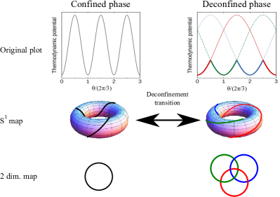
Figure 1: Schematic figures of the topological difference in the confined and deconfined phases with $N_{\mathrm{c}}=3$. The left (right) column represents the confined (deconfined) phase. The first, second and third rows are the original $\theta$-dependence of the thermodynamic potential, its map to $S^{1}$ and its map to 2 dimensional space by replacing the torus. In the right panel of the first row, the bold line represents the global minima. In the second row, solid lines which wind around torus are realized thermodynamic state (global minima of the effective potential) and its $\mathbb{Z}_{3}$ images if those exist.

Here, we plot the thermodynamic states which are global minimum and two possible local minima of the thermodynamic potential at each $\theta$ as lines on the torus. Two possible local minima are so called the $\mathbb{Z}_{3}$ images of the global minimum. In the confined phase, only one line winds around the torus $N_{\mathrm{c}}$ times, but there are $N_{\mathrm{c}}$ lines in the deconfined phase and each line wind around the torus only one time. Number of winding are related with the RW periodicity and its realization mechanism [4, 3]. By removing the torus, lines can be mapped to the 2-dimensional space as closed rings: one ring exists in the confined phase and three entangled rings appear in the deconfined phase. These entangled rings are not the Borromean rings because we cannot untangle them by removing one ring.

To see more topological properties of thermodynamic states, we consider three operations, $\Theta$, $\Upsilon$ and $\mathbb{Z}_{\mathrm{N_{c}}}$, for the thermodynamic state. We set the global minimum of the thermodynamic potential at $\theta=0$ as the initial thermodynamic state and express it as $\psi(\theta=0,\phi=0)$ where $\phi$ represents the phase of the Polyakov loop. In the case with $\mathrm{N}_{c}=3$, $\phi$ can take $0,2\pi/3$ and $4\pi/3$ in the deconfined phase. Three operations are following: ($\Theta$ operation) It shifts $\psi(\theta,\phi)$ to $\psi(\theta+2\pi,\phi^{\prime})$ and then we trace the state which thermodynamic potential decreases if states intersect each other when $\theta$ is varying. ($\Upsilon$ operation) It shifts $\psi(\theta,\phi)$ to $\psi(\theta+2\pi/N_{\mathrm{c}},\phi)$. It can be interpreted that the certain flux is inserted to the closed Euclidean temporal coordinate loop and then $\theta$ is shifted by the Aharonov-Bohm effect. ($\mathbb{Z}_{\mathrm{N_{c}}}$ operation) It is the standard $\mathbb{Z}_{\mathrm{N_{c}}}$ transformation which changes $\psi(\theta,\phi)$ to $\psi(\theta,\phi+2\pi/N_{\mathrm{c}})$ if the $\mathbb{Z}_{\mathrm{N_{c}}}$ images exist. In the confined phase, these operations should commute with each other because thermodynamic states at any $\theta$ belong to the same image as shown in the left-top panel of Fig. 1. By comparison, three operations are not always commutable in the deconfined phase and these show non-trivial commutation relations.

The topological determination of the deconfinement phase transition is not yet applied to nonzero $\mu_{\mathrm{R}}$ region and thus we investigate this region in this paper by using the effective model approach. At finite $\mu_{\mathrm{R}}$, there is the sign problem in the lattice QCD simulation and thus we cannot obtain reliable results. Therefore, the effective model calculations are important to have qualitative and quantitative understanding of the QCD phase structure. To describe the non-trivial free-energy degeneracy correctly, effective models should possess several topological properties of QCD at finite $\theta$. Such effective models sometimes have the model sign problem [8, 9] which, of course, relates with the original sign problem. The model sign problem can be resolved by using the Lefschetz-thimble path-integral method [10, 11, 12] and then we may investigate $\mu_{\mathrm{R}}$ region directly [9], but it is not an easy task at present. We need some more technical extensions of Ref. [9] in the complex $\mu$ case. It should be noted that we can not use the standard approximation for the model sign problem in the PNJL model which only takes into account the real part of the thermodynamics potential in the present case. This approximation restricts $\Phi$ to only take real values. At finite $\mu_{\mathrm{I}}$, the phase of $\Phi$ plays a crucial role and thus it is necessary that $\Phi$ can take complex values.

In this paper, we consider $\mu_{\mathrm{iso}}$ as an alternative approach to investigate the QCD phase structure at finite $\mu_{\mathrm{R}}$. It is because phase diagrams at finite $\mu_{\mathrm{R}}$ and $\mu_{\mathrm{iso}}$ are identical outside of the pion condensed region in the large-$N_{\mathrm{c}}$ limit via the well-known orbifold equivalence [13, 14, 15].

This paper is organized as follows. In the next section, we explain the isospin chemical potential and formulation of the effective model. Numerical results are shown in Sec. 3 Section 4 is devoted to summary.

2 Effective model with isospin chemical potential

In this paper, we consider $\mu_{\mathrm{iso}}$ to extract information of the $\mu_{\mathrm{R}}$ region because the $\mu_{\mathrm{iso}}$ region has following two characteristic properties:

1. Sign problem free

It is well known that there is no sign problem because the condition $\tau_{2}\gamma_{5}{\cal D}\gamma_{5}\tau_{2}={\cal D}^{\dagger}$ is manifested where ${\cal D}$ denotes the Dirac operator and the symbol $\tau_{i}$ mean Pauli matrices in the flavor space. This leads the condition $\mathrm{det}({\cal D})\geq 0$ even if $\mu_{\mathrm{I}}$ is nonzero.

2. Orbifold equivalence

The phase structure at finite $\mu_{\mathrm{iso}}$ is identical with that at finite $\mu_{\mathrm{R}}$ outside of the pion-condensed phase at least in the large-$N_{\mathrm{c}}$ limit [15]. This equivalence is violated with finite $N_{\mathrm{c}}$ by $1/N_{\mathrm{c}}$ corrections such as the flavor mixing loops.

With the two properties, we can expect that the qualitative information of QCD phase diagram at finite $\mu_{\mathrm{R}}$ can be extracted from the QCD phase diagram at finite $\mu_{\mathrm{iso}}$. For example, the no-go theorem of critical phenomena were obtained in Ref. [16] via the orbifold equivalence. The mean-field approximation which picks up the leading-order of the $1/N_{\mathrm{c}}$ expansion is widely used in the effective model calculation to investigate the QCD phase structure and thus our analysis based on the orbifold equivalence can be acceptable for a first step of the issue to understand the topological deconfinement transition at finite $\mu_{\mathrm{R}}$. Therefore, our results may provide positive motivation to perform the lattice QCD simulation in the $\mu_{\mathrm{iso}}\in\mathbb{R}$ region with finite $\mu_{\mathrm{I}}$. It should be noted that the sign problem comes back if we consider the different $\theta$ for two quark fields with different flavor. In this case, the imaginary part of $\mu_{\mathrm{iso}}$ appears in addition to its real part and then the condition, $\tau_{2}\gamma_{5}{\cal D}\gamma_{5}\tau_{2}={\cal D}^{\dagger}$, is no longer valid. This issue does not affect our present discussions, but it should be considered when we take into account the imaginary part of $\mu_{\mathrm{iso}}$ in the future.

To investigate the phase structure at finite $T$ and $\mu_{\mathrm{iso}}$, we use the Polyakov-loop extended Nambu–Jona-Lasinio (PNJL) model [17]. This model can well reproduce the QCD properties at finite $\theta$; see Ref. [18] as an example. The Lagrangian density of the two-flavor and three-color PNJL model in the Euclidean space is

$${\cal L} ={\bar{q}}({\ooalign{\hfil/\hfil\crcr$D$}}+m_{0})-G[({\bar{q}}q)^{2}+({\bar{q}}i\gamma_{5}{\vec{\tau}}q)^{2}]+{\cal V}_{\mathrm{g}}(\Phi,{\bar{\Phi}}),$$ (5)

where $m_{0}$ means the current quark mass, the covariant derivative is $D_{\nu}-igA_{\nu}\delta_{\nu 4}$, $\Phi$ (${\bar{\Phi}}$) denotes the Polyakov-loop (its conjugate) and ${\cal V}_{\mathrm{g}}$ expresses the gluonic contribution. In the case with $m_{0}=\mu_{\mathrm{iso}}=0$, the Lagrangian density has $SU(2)_{L}\times SU(2)_{R}\times U(1)_{V}\times SU(3)_{\mathrm{color}}$ symmetry. With $m_{0}\neq 0$ and $\mu_{\mathrm{I}}\neq 0$, the Lagrangian density has $U(1)_{{\bf I}_{3}}\times U(1)_{V}\times SU(3)_{\mathrm{color}}$ symmetry. For example, see Refs. [19, 20, 21, 22] for recent progress in the investigation of QCD phase structure at finite $\mu_{\mathrm{iso}}$.

The imaginary and isospin chemical potentials can be introduced to the model as the form

$$\mu=\mu_{q}{\bf I}+\mu_{\mathrm{iso}}\tau_{3},$$ (6)

where ${\bf I}$ is the unit matrix. Each $\mu_{q}$ and $\mu_{\mathrm{iso}}$ can be represented as

$$\mu_{q}=\frac{\mu_{u}+\mu_{d}}{2},~{}~{}~{}~{}\mu_{\mathrm{iso}}=\frac{\mu_{u}-\mu_{d}}{2},$$ (7)

where $\mu_{u}$ ($\mu_{d}$) is the quark chemical potential of up (down) quark. In this paper, we consider $\mu_{q}=i\mu_{\mathrm{I}}$ ($\mu_{\mathrm{I}}\in\mathbb{R}$) and $\mu_{\mathrm{iso}}\in\mathbb{R}$ to discuss the topological deconfinement transition at finite $\mu_{\mathrm{iso}}$.

With the mean-field approximation, the thermodynamic potential can be expressed as

$${\cal V} ={\cal V}_{\mathrm{f}}+{\cal V}_{\mathrm{g}},$$ (8)

where ${\cal V}_{\mathrm{f,g}}$ are the fermionic and gluonic parts, respectively. The actual form of ${\cal V}_{\mathrm{f}}$ is

$${\cal V}_{\mathrm{f}} =-2\sum_{i=\pm}\int\frac{d^{3}p}{(2\pi)^{3}}\Bigl{[}3E_{i,{\bf p}}+T\ln\Bigl{(}f_{i}^{-}f_{i}^{+}\Bigr{)}\Bigr{]}$$

$$+G(\sigma^{2}+\pi^{2}),$$ (9)

where

$$f^{-}_{i} =1+3(\Phi+{\bar{\Phi}}e^{-\beta E_{i,{\bf p}}^{-}})e^{-\beta E_{i,{\bf p}}^{-}}+e^{-3\beta E_{i,{\bf p}}^{-}},$$

$$f^{+}_{i} =1+3({\bar{\Phi}}+\Phi e^{-\beta E_{i,{\bf p}}^{+}})e^{-\beta E_{i,{\bf p}}^{+}}+e^{-3\beta E_{i,{\bf p}}^{+}}.$$ (10)

Quark single particle energies are given as $E_{\pm{\bf p}}^{\mp}=E_{\pm}\mp i\mu_{\mathrm{I}}$ with $E_{\pm}=\sqrt{(E_{\bf p}\pm\mu_{\mathrm{iso}})^{2}+N^{2}}$ for $E_{\bf p}=\sqrt{{\bf p}^{2}+M^{2}}$. Symbols $M$ and $N$ are defined as $M=m_{0}-2G\sigma$ and $N=-2G\pi$ with $\sigma=\langle{\bar{q}}q\rangle$ and $\pi=\langle{\bar{q}}i\gamma_{5}\tau_{1}q\rangle$. Here we take the order parameter of the $U(1)_{{\bf I}_{3}}$ symmetry breaking as

$$\pi^{\pm}=\frac{1}{\sqrt{2}}e^{\pm i\varphi}=\langle{\bar{q}}i\gamma_{5}\tau_{\pm}q\rangle,$$ (11)

and we can set $\varphi=0$ as in Ref. [23, 24] without loss of generality. In the following disucssions, we set $\pi=|\langle{\bar{q}}i\gamma_{5}\tau_{1}q\rangle|$. For example, see Ref. [23, 25, 26] for discussions in the isospin chemical potential region by using the NJL model.

We employ the Polyakov loop potential used in Ref. [27] as ${\cal V}_{\mathrm{g}}$ and the parameter set used in Ref. [28]; for details of the PNJL model with $\mu_{\mathrm{iso}}$, see Refs. [24, 29, 28] as an example. In the PNJL model, the model Polyakov-loop is defined as

$$\Phi =\frac{1}{N_{\mathrm{c}}}\mathrm{tr}_{c}\Bigl{[}e^{ig\langle A_{4}\rangle/T}\Bigr{]},$$ (12)

with the Polyakov-gauge fixing. The Polyakov loop is, of course, gauge invariant, but Eq. (12) is not; see Ref. [30] for discussions on the model and correct Polyakov-loops from the Jensen inequality. Nevertheless, the model Polyakov loop Eq. (12) is enough for our purpose. The Polyakov loop is introduced to just model the $\mathbb{Z}_{3}$ properties of QCD because the modeling of $\mathbb{Z}_{3}$ properties plays a crucial role to reproduce characteristic properties of QCD at finite $\theta$. Thus, there is no need to reproduces the correct Polyakov-loop by the model Polyakov-loop. It is the reason why we use the simplest PNJL model in this paper.

The PNJL model seems to be an adequate effective model to describe the topological properties of QCD at finite $\mu_{\mathrm{I}}$ and thus it allows us to discuss the topological confinement-deconfinement transition. Our numerical results presented in the next section are performed in the situation that the topological confinement-deconfinement transition is modeled at $\mu_{\mathrm{R}}=0$ and after the $\mu_{\mathrm{iso}}$-dependence of the transition is discussed. It should be noted that we do not claim that the PNJL model can reproduce all of QCD properties.

3 Numerical results

To investigate the topological deconfinement transition, $\theta=\pi/3$ region is important as shown in Eq. (2) and thus we show the quark number density at $\theta=\pi/3$ in addition to the chiral condensate, the pion condensate and the Polyakov loop at $\theta=0$ here. Figure 2 shows $|\sigma|/m_{\pi}^{3}$, $\pi/m_{\pi}^{3}$, $|\Phi|$ and $|n_{q}|/m_{\pi}^{3}$ as a function of $T/m_{\pi}$ and $\mu_{\mathrm{iso}}/m_{\pi}$.

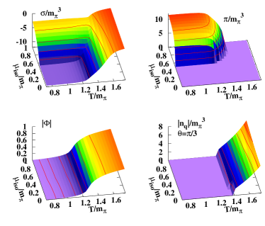
Figure 2: The $T$ and $\mu_{\mathrm{iso}}$ dependence of the chiral condensate, the pion condensate and the Polyakov loop at $\theta=0$ and the quark number density at $\theta=\pi/3$. Quantities are normalized by $m_{\pi}=138$ [MeV].

The chiral and pion condensates strongly depend on $\mu_{\mathrm{iso}}$ as well as on $T$, but the Polyakov loop and the quark number density are less sensitive to $\mu_{\mathrm{iso}}$. In the leading-order approximation of the PNJL model, the gluonic contributions do not have the explicit chemical-potential dependence because there is no quark polarization effects which are higher order contributions of the $1/N_{\mathrm{c}}$ expansion. Thus, $\mu_{\mathrm{iso}}$ cannot affect the Polyakov loop directly. It is interesting to compare these results with the isospin-density dependence of the Polyakov-loop on the lattice [19]. Interesting point is that the quark number density is also insensitive to $\mu_{\mathrm{iso}}$ and it means that the chiral and deconfinement transition are not correlated strongly. This tendency can be expected to appear at finite $\mu_{\mathrm{R}}$ via the orbifold equivalence outside of the pion-condensed phase.

In the topological determination of the confinement-deconfinement transition, the behavior of quark number density at finite $\theta$ is important. The left (right) panel of Fig. 3 shows the behavior of $n_{q}$ as a function of $\theta$ with $\mu_{\mathrm{iso}}=0$ ($0.8m_{\pi}$) for $T=160$, $180$ and $200$ MeV. The $\theta$ dependence of the quark number density clearly shows the general feature of the topological phase transition discussed in Sec. 1: It is smooth below $T_{\mathrm{RW}}$ and has gaps above $T_{\mathrm{RW}}$. By comparison, the quark number density does not strongly depend on $\mu_{\mathrm{iso}}$. This behavior means that the topological confinement-deconfinement temperature is not very sensitive to $\mu_{\mathrm{iso}}$ in the present model.

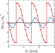
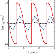
Figure 3: The $\theta$ dependence of the quark number density with $\mu_{\mathrm{iso}}=0$ and $0.8m_{\pi}$. The dotted, dashed and solid lines are results at $T=160$, $180$ and $200$ MeV, respectively.

For reader’s convenience, we also show the $T/m_{\pi}$ dependence of $|\sigma|/\sigma_{0}$, $\pi/\sigma_{0}$ and $\Phi$ at $\theta=0$ and $|n_{q}|/\sigma_{0}$ at $\theta=\pi/3$ with $\mu_{\mathrm{iso}}/m_{\pi}=0,0.4,0.6,1$ in Fig. 4.

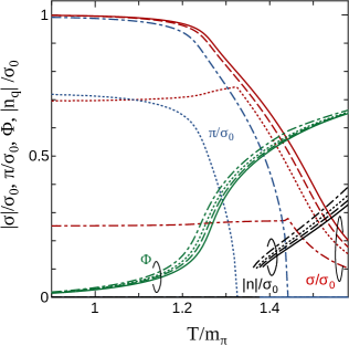
Figure 4: The $T$ dependence of the chiral condensate, the pion condensate and the Polyakov loop at $\theta=0$ and the quark number density at $\theta=\pi/3$. The solid, dashed, dotted, and dot-dashed lines are these quantities at $\mu_{\mathrm{iso}}/m_{\pi}=0,0.4,0.6,\mathrm{and}\ 1$, respectively. Quantities are normalized by $\sigma_{0}=|\sigma_{\mathrm{vacuum}}|$. The step-size of $T$ is 1 [MeV].

The phase diagram in the $(T,\mu_{\mathrm{iso}})$ plane is shown in Fig. 5.

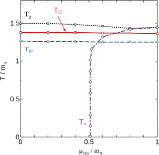
Figure 5: The phase diagram in the $T$-$\mu_{\mathrm{iso}}$ plane. Symbols are numerical results and lines are linear interpolations between them. The solid, dashed, dotted and dot-dashed lines are explained in the text. Numerical error of these lines are about $\pm 1.5$ [MeV].

The solid, dashed, dotted and dot-dashed lines are the deconfinement transition temperature ($T_{\mathrm{D}}$), the deconfinement pseudo-critical temperature determined by the peak of $d\Phi/dT$ ($T_{\Phi}$), the chiral pseudo-critical temperature determined by the peak of $d\sigma/dT$ ($T_{\chi}$) and the phase transition temperature of the pion condensation ($T_{\pi}$). If $d\sigma/dT$ and $d\Phi/dT$ have two peaks, we choice higher one as the pseudo-critical temperature. We determine $T_{\mathrm{D}}$ by $T_{\mathrm{RW}}$ in this paper because the triple-point nature of the RW endpoint depends on the form of ${\cal V}_{\mathrm{g}}$ in the PNJL model and also the qualitative behavior of $T_{\mathrm{RW}}$ and $T_{\mathrm{Beard}}$ are basically same. From Fig. 5, we can find following features:

1. Behavior of $\mathbf{T_{D}}$ and $\mathbf{T_{\Phi}}$

$T_{\mathrm{D}}$ and $T_{\Phi}$ slightly decrease with increasing $\mu_{\mathrm{iso}}$ and show similar qualitative behaviors. However, $\Phi$ is continuously changed at finite $T$ and thus the determination of $T_{\Phi}$ is not clear unlike $T_{\mathrm{D}}$.

2. Behavior of $\mathbf{T_{D}}$ at finite density

$T_{\mathrm{D}}$ decreases with increasing $\mu_{\mathrm{iso}}$ and thus we can expect that $T_{\mathrm{D}}$ also show decreasing behavior at finite $\mu_{\mathrm{R}}$ via the orbifold equivalence. This result is consistent with our perturbative estimate of $T_{D}$ at small $\mu_{\mathrm{R}}$ [3].

3. Relation between $\mathbf{T_{D}}$ and $\mathbf{T_{\chi}}$

The present definition of $T_{D}$ is not affected much by the chiral transition even though we use the quark-bilinear $\langle{q^{\dagger}q}\rangle$.

4. Relation between $\mathbf{T_{D}}$ and $\mathbf{T_{\pi}}$

By comparison, $T_{D}$ seems to be smaller than $T_{\pi}$ at large $\mu_{\mathrm{iso}}$. This is not unreasonable since these transition are independent of each other. Finite quark mass leaves $\sigma$ finite and pion keeps its Nambu-Goldstone boson nature even at large $T$. For example, some effective model results including the present one show $T_{\chi}>T_{\mathrm{D}}$ at $\mu_{\mathrm{R}}=0$.

We also note that $T_{D}$ is smaller than $T_{\chi}$ at small $\mu_{\mathrm{iso}}$. When the pseudo-critical chiral transition boundary ends at the RW endpoint, one should find $T_{\chi}(\theta=0)<T_{\chi}(\theta=\pi/3)=T_{\mathrm{RW}}(=T_{D})$. It should be noted that this is not always the case; the order of two temperatures, $T_{\chi}$ and $T_{\mathrm{RW}}$, depends on the details of the framework. In the present setup, the chiral transition boundary reaches the RW transition line ($\theta=\pi/3$) at significantly higher temperature than the RW endpoint, $T_{\chi}(\theta=\pi/3)>T_{\mathrm{RW}}$. It should be noted that the difference between the confinement-deconfinement temperatures determined from $T_{\mathrm{RW}}$ and $T_{\mathrm{Beard}}$ are almost the same in the present model. We check it at $\mu_{\mathrm{iso}}=0$ and $0.8m_{\pi}$. Actually, the difference, $(T_{\mathrm{RW}}-T_{\mathrm{Beard}})/T_{\mathrm{RW}}$, is less than $3$% and the slightly decreasing behavior of $T_{\mathrm{Beard}}$ with increasing $\mu_{\mathrm{iso}}$ also appears.

Sensitivity of the critical temperature on the chemical potential is quantified using the curvature $\kappa$,

$$\frac{T_{c}(\mu)}{T_{c}(\mu=0)}=1-\kappa\,\left(\frac{N_{\mathrm{c}}\mu}{T}\right)^{2}+\mathcal{O}\left[\left(\frac{N_{\mathrm{c}}\mu}{T}\right)^{4}\right]\ .$$ (13)

For $T_{c}=T_{\chi},T_{\Phi}$ and $T_{\mathrm{D}}$ with $\mu=\mu_{\mathrm{iso}}$, the curvatures are obtained as $\kappa_{\chi}=0.017\pm 0.001$, $\kappa_{\Phi}=0.004\pm 0.001$ and $\kappa_{\mathrm{D}}=0.003\pm 0.001$, respectively. Compared with the chiral transition, curvatures in $T_{\Phi}$ and $T_{D}$ are much smaller, and show that the deconfinement temperature is much less sensitive to $\mu_{\mathrm{iso}}$ than the chiral transition temperature. The chiral transition curvature is larger than the lattice result in the real quark chemical potential, $\kappa\simeq 0.008$ [31], but it is within a two sigma uncertainty of more recent lattice results $\kappa=0.013\pm 0.003$ [32], $\kappa=0.0135\pm 0.002$ [33], $\kappa=0.0149\pm 0.0021$ [34] and $\kappa=0.020\pm 0.004$ [35]. The agreement would be accidental, but suggests the validity of the orbifold equivalence.

4 Summary

In this paper, we have discussed the deconfinement transition from topological viewpoints. Modification of the topology of the system is achieved by introducing the dimensionless imaginary chemical potential ($\theta$).

The topological difference between the confined and deconfined is visualized by using the map of the thermodynamic quantities to circle $S^{1}$ along periodic $\theta$. Then, we find that there are three entangled rings of thermodynamic states in the deconfined phase, but there is only one ring in the confined phase after performing the $2$-dimensional map of thermodynamic states. To understand it more clearly, we have considered three operations for the thermodynamic state, $\theta$ shift, the flux insertion to the closed Euclidean temporal coordinate loop and $\mathbb{Z}_{\mathrm{N_{c}}}$ transformation, and found nontrivial commutation relations between them in the deconfined phase.

To investigate the topological deconfinement phase transition in the real chemical potential ($\mu_{\mathrm{R}}$) region, we have investigated the isospin chemical potential ($\mu_{\mathrm{iso}}$) region. Phase diagrams in both regions are identical to each other outside of the pion-condensed phase via the orbifold equivalence at least in the large-$N_{\mathrm{c}}$ limit. The chiral and pion condensates are strongly affected by $\mu_{\mathrm{iso}}$, but the Polyakov-loop and the quark number density at $\theta=\pi/3$ are not. We show this feature by estimating the curvature of transition lines. In the present PNJL model treatment, the gluonic part does not have explicit chemical potential dependence because the quark polarization effects are ignored. This leads to uncorrelated results between the chiral and deconfinement transitions. Some results for the chiral and pion condensations have been observed on the lattice [36, 37, 38, 39, 40, 19, 20], but not for the quark number density at $\theta=\pi/3$. If we will access lattice QCD data of the quark number density at finite $\mu_{\mathrm{iso}}$ with $\theta=\pi/3$ in the future, we can judge our surmise. If lattice simulations will provide the strong correlated results between the chiral and the deconfinement transitions at finite $\mu_{\mathrm{iso}}$, we can use the $\mu_{\mathrm{iso}}$ region as a laboratory to extend the gluonic part of the effective model to include quark polarization effects by comparing the deconfinement transition in the effective model and that in lattice QCD simulations.

In this study, we clarify topological properties of QCD via the imaginary chemical potential. Also, it is a first study of the topological deconfinement transition at finite chemical potential. We hope that this study shed a light to nature of the deconfinement transition from topological viewpoint. One of the possible future directions of this study is the calculation of the Uhlmann phase [41] which has been used to discuss the finite temperature topological-order in the condensed matter physics [42, 43]. Therefore, we can clarify the confinement-deconfinement transition from the same context of the condensed matter physics if we can calculate the Uhlmann phase in QCD. The calculation of the Uhlmann phase in QCD seems to be very difficult or impossible at present, but it will complete our discussions presented in Refs. [3, 5] and also this paper.

The authors thank H. Kouno for his useful comments. K.K. is supported by Grant-in-Aid for Japan Society for the Promotion of Science (JSPS) fellows No.26-1717. A.O. is supported in part by the Grants-in-Aid for Scientific Research from JSPS (Nos. 15K05079, 15H03663, 16K05350), the Grants-in-Aid for Scientific Research on Innovative Areas from MEXT (Nos. 24105001, 24105008), and by the Yukawa International Program for Quark-hadron Sciences (YIPQS).

References

- [1] M. Sato, Topological discrete algebra, ground state degeneracy, and quark confinement in QCD, Phys.Rev. D77 (2008) 045013. arXiv:0705.2476, doi:10.1103/PhysRevD.77.045013.
- [2] X. Wen, Topological Order in Rigid States, Int.J.Mod.Phys. B4 (1990) 239. doi:10.1142/S0217979290000139.
- [3] K. Kashiwa, A. Ohnishi, Topological feature and phase structure of QCD at complex chemical potential, Phys. Lett. B750 (2015) 282–286. arXiv:1505.06799, doi:10.1016/j.physletb.2015.09.036.
- [4] A. Roberge, N. Weiss, Gauge Theories With Imaginary Chemical Potential and the Phases of QCD, Nucl.Phys. B275 (1986) 734. doi:10.1016/0550-3213(86)90582-1.
- [5] K. Kashiwa, A. Ohnishi, Quark number holonomy and confinement-deconfinement transition, Phys. Rev. D93 (11) (2016) 116002. arXiv:1602.06037, doi:10.1103/PhysRevD.93.116002.
- [6] M. D’Elia, F. Sanfilippo, The Order of the Roberge-Weiss endpoint (finite size transition) in QCD, Phys. Rev. D80 (2009) 111501. arXiv:0909.0254, doi:10.1103/PhysRevD.80.111501.
- [7] C. Bonati, G. Cossu, M. D’Elia, F. Sanfilippo, The Roberge-Weiss endpoint in QCD, Phys.Rev. D83 (2011) 054505. arXiv:1011.4515, doi:10.1103/PhysRevD.83.054505.
- [8] K. Fukushima, Y. Hidaka, A Model study of the sign problem in the mean-field approximation, Phys.Rev. D75 (2007) 036002. arXiv:hep-ph/0610323, doi:10.1103/PhysRevD.75.036002.
- [9] Y. Tanizaki, H. Nishimura, K. Kashiwa, Evading the sign problem in the mean-field approximation through Lefschetz-thimble path integral, Phys. Rev. D91 (10) (2015) 101701. arXiv:1504.02979, doi:10.1103/PhysRevD.91.101701.
- [10] E. Witten, Analytic Continuation Of Chern-Simons Theory, AMS/IP Stud. Adv. Math. 50 (2011) 347–446. arXiv:1001.2933.
- [11] M. Cristoforetti, F. Di Renzo, L. Scorzato, New approach to the sign problem in quantum field theories: High density QCD on a Lefschetz thimble, Phys.Rev. D86 (2012) 074506. arXiv:1205.3996, doi:10.1103/PhysRevD.86.074506.
- [12] H. Fujii, D. Honda, M. Kato, Y. Kikukawa, S. Komatsu, T. Sano, Hybrid Monte Carlo on Lefschetz thimbles - A study of the residual sign problem, JHEP 1310 (2013) 147. arXiv:1309.4371, doi:10.1007/JHEP10(2013)147.
- [13] A. Cherman, M. Hanada, D. Robles-Llana, Orbifold equivalence and the sign problem at finite baryon density, Phys. Rev. Lett. 106 (2011) 091603. arXiv:1009.1623, doi:10.1103/PhysRevLett.106.091603.
- [14] A. Cherman, B. C. Tiburzi, Orbifold equivalence for finite density QCD and effective field theory, JHEP 06 (2011) 034. arXiv:1103.1639, doi:10.1007/JHEP06(2011)034.
- [15] M. Hanada, N. Yamamoto, Universality of Phases in QCD and QCD-like Theories, JHEP 1202 (2012) 138. arXiv:1103.5480, doi:10.1007/JHEP02(2012)138.
- [16] Y. Hidaka, N. Yamamoto, No-Go Theorem for Critical Phenomena in Large-Nc QCD, Phys.Rev.Lett. 108 (2012) 121601. arXiv:1110.3044, doi:10.1103/PhysRevLett.108.121601.
- [17] K. Fukushima, Chiral effective model with the Polyakov loop, Phys.Lett. B591 (2004) 277–284. arXiv:hep-ph/0310121, doi:10.1016/j.physletb.2004.04.027.
- [18] Y. Sakai, K. Kashiwa, H. Kouno, M. Yahiro, Polyakov loop extended NJL model with imaginary chemical potential, Phys.Rev. D77 (2008) 051901. arXiv:0801.0034, doi:10.1103/PhysRevD.77.051901.
- [19] G. Endrödi, Magnetic structure of isospin-asymmetric QCD matter in neutron stars, Phys. Rev. D90 (9) (2014) 094501. arXiv:1407.1216, doi:10.1103/PhysRevD.90.094501.
-
[20]
B. B. Brandt, G. Endrodi,
QCD
phase diagram with isospin chemical potential, in: Proceedings, 34th
International Symposium on Lattice Field Theory (Lattice 2016): Southampton,
UK, July 24-30, 2016, 2016.
arXiv:1611.06758.
URL https://inspirehep.net/record/1499491/files/arXiv:1611.06758.pdf - [21] T. Brauner, X.-G. Huang, Vector meson condensation in a pion superfluid, Phys. Rev. D94 (9) (2016) 094003. arXiv:1610.00426, doi:10.1103/PhysRevD.94.094003.
- [22] G. Cao, L. He, X.-G. Huang, A quarksonic matter at high isospin densityarXiv:1610.06438.
- [23] L.-y. He, M. Jin, P.-f. Zhuang, Pion superfluidity and meson properties at finite isospin density, Phys. Rev. D71 (2005) 116001. arXiv:hep-ph/0503272, doi:10.1103/PhysRevD.71.116001.
- [24] Z. Zhang, Y.-X. Liu, Coupling of pion condensate, chiral condensate and Polyakov loop in an extended NJL model, Phys. Rev. C75 (2007) 064910. arXiv:hep-ph/0610221, doi:10.1103/PhysRevC.75.064910.
- [25] G.-f. Sun, L. He, P. Zhuang, BEC-BCS crossover in the Nambu-Jona-Lasinio model of QCD, Phys. Rev. D75 (2007) 096004. arXiv:hep-ph/0703159, doi:10.1103/PhysRevD.75.096004.
- [26] L. He, M. Jin, P. Zhuang, Pion Condensation in Baryonic Matter: from Sarma Phase to Larkin-Ovchinnikov-Fudde-Ferrell Phase, Phys. Rev. D74 (2006) 036005. arXiv:hep-ph/0604224, doi:10.1103/PhysRevD.74.036005.
- [27] S. Roessner, C. Ratti, W. Weise, Polyakov loop, diquarks and the two-flavour phase diagram, Phys.Rev. D75 (2007) 034007. arXiv:hep-ph/0609281, doi:10.1103/PhysRevD.75.034007.
- [28] H. Kouno, M. Kishikawa, T. Sasaki, Y. Sakai, M. Yahiro, Spontaneous parity and charge-conjugation violations at real isospin and imaginary baryon chemical potentials, Phys. Rev. D85 (2012) 016001. arXiv:1110.5187, doi:10.1103/PhysRevD.85.016001.
- [29] S. Mukherjee, M. G. Mustafa, R. Ray, Thermodynamics of the PNJL model with nonzero baryon and isospin chemical potentials, Phys. Rev. D75 (2007) 094015. arXiv:hep-ph/0609249, doi:10.1103/PhysRevD.75.094015.
- [30] J. Braun, H. Gies, J. M. Pawlowski, Quark Confinement from Color Confinement, Phys.Lett. B684 (2010) 262–267. arXiv:0708.2413, doi:10.1016/j.physletb.2010.01.009.
- [31] C. R. Allton, S. Ejiri, S. J. Hands, O. Kaczmarek, F. Karsch, E. Laermann, C. Schmidt, L. Scorzato, The QCD thermal phase transition in the presence of a small chemical potential, Phys. Rev. D66 (2002) 074507. arXiv:hep-lat/0204010, doi:10.1103/PhysRevD.66.074507.
- [32] C. Bonati, M. D’Elia, M. Mariti, M. Mesiti, F. Negro, F. Sanfilippo, Curvature of the chiral pseudocritical line in QCD, Phys. Rev. D90 (11) (2014) 114025. arXiv:1410.5758, doi:10.1103/PhysRevD.90.114025.
- [33] C. Bonati, M. D’Elia, M. Mariti, M. Mesiti, F. Negro, F. Sanfilippo, Curvature of the chiral pseudocritical line in QCD: Continuum extrapolated results, Phys. Rev. D92 (5) (2015) 054503. arXiv:1507.03571, doi:10.1103/PhysRevD.92.054503.
- [34] R. Bellwied, S. Borsanyi, Z. Fodor, J. Günther, S. D. Katz, C. Ratti, K. K. Szabo, The QCD phase diagram from analytic continuation, Phys. Lett. B751 (2015) 559–564. arXiv:1507.07510, doi:10.1016/j.physletb.2015.11.011.
- [35] P. Cea, L. Cosmai, A. Papa, Critical line of 2+1 flavor QCD: Toward the continuum limit, Phys. Rev. D93 (1) (2016) 014507. arXiv:1508.07599, doi:10.1103/PhysRevD.93.014507.
- [36] J. B. Kogut, D. K. Sinclair, Quenched lattice QCD at finite isospin density and related theories, Phys. Rev. D66 (2002) 014508. arXiv:hep-lat/0201017, doi:10.1103/PhysRevD.66.014508.
- [37] J. B. Kogut, D. K. Sinclair, Lattice QCD at finite isospin density at zero and finite temperature, Phys. Rev. D66 (2002) 034505. arXiv:hep-lat/0202028, doi:10.1103/PhysRevD.66.034505.
- [38] J. B. Kogut, D. K. Sinclair, The Finite temperature transition for 2-flavor lattice QCD at finite isospin density, Phys. Rev. D70 (2004) 094501. arXiv:hep-lat/0407027, doi:10.1103/PhysRevD.70.094501.
- [39] P. de Forcrand, M. A. Stephanov, U. Wenger, On the phase diagram of QCD at finite isospin density, PoS LAT2007 (2007) 237. arXiv:0711.0023.
- [40] W. Detmold, K. Orginos, Z. Shi, Lattice QCD at non-zero isospin chemical potential, Phys. Rev. D86 (2012) 054507. arXiv:1205.4224, doi:10.1103/PhysRevD.86.054507.
- [41] A. Uhlmann, Parallel Transport and Quantum Holonomy along Density Operators, Rep. Math. Phys. 24 (1986) 229. doi:10.1016/0034-4877(86)90055-8.
- [42] O. Viyuela, A. Rivas, M. Martin-Delgado, Uhlmann Phase as a Topological Measure for One-Dimensional Fermion Systems, Phys.Rev.Lett. 112 (2014) 130401. arXiv:1309.1174, doi:10.1103/PhysRevLett.112.130401.
- [43] O. Viyuela, A. Rivas, M. Martin-Delgado, Two-dimensional density-matrix topological fermionic phases: Topological uhlmann numbers, Physical review letters 113 (7) (2014) 076408.