This paper presents an alternative approach to p-values in regression settings. This approach, whose origins can be traced to machine learning, is based on the leave-one-out bootstrap for prediction error. In machine learning this is called the out-of-bag (OOB) error. To obtain the OOB error for a model, one draws a bootstrap sample and fits the model to the in-sample data. The out-of-sample prediction error for the model is obtained by calculating the prediction error for the model using the out-of-sample data. Repeating and averaging yields the OOB error, which represents a robust cross-validated estimate of the accuracy of the underlying model. By a simple modification to the bootstrap data involving “noising up” a variable, the OOB method yields a variable importance (VIMP) index, which directly measures how much a specific variable contributes to the prediction precision of a model. VIMP provides a scientifically interpretable measure of the effect size of a variable, we call the predictive effect size, that holds whether the researcher’s model is correct or not, unlike the p-value whose calculation is based on the assumed correctness of the model. We also discuss a marginal VIMP index, also easily calculated, which measures the marginal effect of a variable, or what we call the discovery effect. The OOB procedure can be applied to both parametric and nonparametric regression models and requires only that the researcher can repeatedly fit their model to bootstrap and modified bootstrap data. We illustrate this approach on a survival data set involving patients with systolic heart failure and to a simulated survival data set where the model is incorrectly specified to illustrate its robustness to model misspecification.

Keywords: Bootstrap sample; Out-of-bag; Prediction error; Variable importance.

1 Introduction

The issue of p-values has taken center stage in the media with many scientists expressing grave concerns about their validity. “P values, the ’gold standard’ of statistical validity, are not as reliable as many scientists assume”, is the leading assertion of the highly accessed Nature article, “Scientific method: Statistical errors” (Nuzzo, 2014). Even more extreme is the recent action of the journal of Basic and Applied Social Psychology (BASP), which announced it would no longer publish papers containing p-values. In explaining their decision for this policy (Trafimow and Marks, 2015), the editors stated that hypothesis significance testing procedures are invalid, and that p-values have become a crutch for scientists dealing with weak data. These, and other highly visible discussions, so alarmed the American Statistical Association (ASA), that it recently issued a formal statement on p-values (Wasserstein and Lazar, 2016), the first time in its history it had ever issued a formal statement on matters of statistical practice.

A big part of the problem is that researchers want the p-value to be something that it was never designed for. Researchers want to make context specific assertions about their findings; they especially want a statistic that allows them to assert statements regarding scientific effect. Because the p-value cannot do this, and because the terminology is confusing and stifling, this leads to misuse and confusion. Another problem is verifying correctness of the model under which the p-value is calculated. If model assumptions do not hold, the p-value itself becomes statistically invalid. This is not an esoteric point. Commonly used models such as linear regression, logistic regression, and Cox proportional hazards can involve strong assumptions. Common practices such as fitting main effect models without interactions, assuming linearity of variables, and invoking distributional assumptions regarding the data, such as normality, can easily fail to hold. Moreover, the functional relationship between attributes and outcome implicit in some of these models, such as proportionality of hazards, may also fail to hold. Researchers rarely test for model correctness, and even when they do, they invariably do so by considering goodness of fit. But goodnesss of fit measures are notoriously unreliable for assessing the validity of a model (Breiman, 2001a). All of this implies that a researchers’ findings, which hinges so much on the p-value being correct, could be suspect without their even knowing it. This fragility of the p-value is further compounded by other conditions typically outside of the control of the researcher, such as the sample size, which has enormous effect on its efficacy.

In this paper we focus on the use of p-values in the context of regression models. All widely used statistical software provide p-value information when fitting regression models; typically p-values are given for the regression coefficients. These are provided in an ANOVA table with each row of the table displays the regression coefficient estimate, $\hat{\beta}$, for a specific coefficient, $\beta$, an estimate of its standard error, $\hat{\sigma}_{\beta}$, and then finally the p-value of the coefficient, obtained typically by comparing a $Z$-statistic to a normal distribution:

$$Z_{\text{observed}}=\frac{\hat{\beta}}{\hat{\sigma}_{\beta}},\hskip 10.0pt\text{p-value}=P\{Z\geq|Z_{\text{observed}}|\}.$$

The p-value for the regression coefficient represents the statistical significance of the test of the null hypothesis $H_{0}\!\!:\beta=0$. In other words, it provides a means of assessing whether a specific coefficient, in this case $\beta$, is zero. However, there is a subtle aspect to this where confusion can take place. When considering this p-value, it is important to keep in mind that its value is calculated not only under the null hypothesis of a zero coefficient value, but also assuming that the model holds. Thus, technically speaking, the null hypothesis is not just that the coefficient is zero, but is a collection of assorted assumptions, which should probably read something like:

$$H_{0}\!:\,\Bigl{\{}\beta=0,\hskip 3.0pt\text{model holds},\hskip 3.0pt\text{model assumptions hold (e.g.\, interactions not present)}\Bigr{\}}.$$

If any of these assumptions fail to hold, then the p-value is technically invalid.

1.1 Contributions and outline of the article

Given these concerns with the p-value, we suggest a different approach using a quantity we call the variable importance (VIMP) index. Our VIMP index is based on variable importance, an idea that originates from machine learning. One of its earliest examples can be traced to Classification and Regression Trees (CART), where variable importance based on surrogate splitting was used to rank variables (see Chapter 5 of Breiman et al. (1984)). The idea was later refined for variable selection in random forest regression and classification models by using prediction error (Breiman, 2001a, b). Extensions to random survival forests were considered by Ishwaran et al. (2008). Our VIMP index uses the same idea as these latter approaches, but recasts it within the p-value context. Like those methods, it uses prediction error to assess the effect of a variable in a model. It replaces the statistical significance of a p-value with the predictive importance of a variable. Most importantly, the VIMP index holds regardless of whether the model is true. This is because the index is calculated using test data and is not based on a presupposed model being true as the p-value does.

In statistics, effect size is a quantitative measure of the strength of a phenomenon, which includes as examples: Cohen’s $d$ (standard group mean difference); the correlation between two variables; and relative risk. In regression models, effect size is measured by the standardized $\hat{\beta}$ coefficient. Since VIMP is also a measure of the quantitative strength of a variable, we refer to its quantitative measure as predictive effect size to prevent readers from confusing it with the traditional effect size. With a simple modification to the VIMP procedure, we estimate another quantity we call marginal VIMP and refer to its quantitative measure as the discovery effect size. This refers to the discovery contribution of a variable, which will be explained in Section 4. An important aspect of both our procedures is that they can be carried out using the same models the researcher is interested in studying. Implementing them only requires the ability to resample the data, apply some modifications to the data, and calculate prediction error. Thus they can easily be incorporated with most existing statistical software procedures.

Section 2 outlines the VIMP index and provides a formal algorithmic formulation (see Algorithm 1). The VIMP index is based on out-of-bag (OOB) estimation, which relies on bootstrap sampling. These concepts are also discussed in Section 2. Section 3 illustrates the use of the VIMP index to a survival data set involving patients with systolic heart failure with cardiopulmonary stress testing. We show how to use this value to rank risk factors and assess their predictive effect sizes. In Section 4 we discuss the extension to marginal VIMP (Algorithm 2) and show how this can be used to estimate discovery effect sizes in the systolic heart failure example. Section 5 studies how sample size ($n$) effects VIMP, comparing this to p-values to show robustness of VIMP to $n$, then in Section 6 we use a synthetically constructed data set where the model is incorrectly specified to illustrate the robustness of VIMP in misspecified settings. We conclude the paper with a discussion in Section 7.

2 OOB prediction error and VIMP

OOB estimation is a bootstrap technique for estimating the prediction error of a model. While the phrase “out-of-bag” might be unfamiliar to readers, the technique has been known for quite some time in the literature, appearing under various names and seemingly different guises. In the statistical literature, the OOB estimator is refered to as the leave-one-out bootstrap due to its connection to leave-one-out cross-validation (Efron and Tibshirani, 1997). See also the earlier paper by Efron (1983) where a similar idea is discussed. It is also used in machine learning where it is refered to as OOB estimation (Breiman, 1996) due to its connections to the machine learning method, bagging (Breiman, 1996).

Calculating the OOB error begins with bootstrap sampling. A bootstrap sample is a sample of the data obtained by sampling with replacement. Sampling by replacement creates replicated values. On average, a bootstrap sample contains only 63.2% of the original data referred to as in-sample or inbag. The remaining 37% of the data, which is out-of-sample, and called the OOB data, is used as test data in the OOB calculation. The OOB error for a model is obtained by fitting a model to bootstrap data, calculating its test set error on the OOB data, and then repeating this many times ($B$ times), and averaging. More technically, if $\text{Err}_{b}$ is the OOB test set error from the $b$th bootstrap sample, the OOB error is

$$\text{Err}_{\text{oob}}=\frac{1}{B}\sum_{b=1}^{B}\text{Err}_{b}.$$

See Figure 1 for an illustration of calculating OOB error.

Figure 1: Calculating the OOB prediction error for a model. Blue points depict inbag sampled values, red points depict OOB values. Model is fit using inbag data and then tested on OOB test data. Averaging the prediction error over the different bootstrap realizations yields the OOB prediction error.

2.1 Calculating the VIMP index for a variable

The VIMP index for a variable $v$ is obtained by a slight extension to the above procedure. When calculating the OOB error for a model, the OOB data for variable $v$ is “noised up”. Noising the OOB data is intended to destroy the association between $v$ and the outcome. Using the altered OOB data, one calculates the prediction error for the model, call this $\text{Err}_{v,b}$ ($b$ is the specific bootstrap sample). The VIMP index $\Delta_{v,b}$ is the difference between this and the prediction error for the original OOB data, $\text{Err}_{b}$. This value will be positive if $v$ is predictive because the prediction error for the noised up data will increase relative to the original prediction error. Averaging $\Delta_{v,b}$ yields the VIMP index, $\Delta_{v}$,

$$\Delta_{v}=\frac{1}{B}\sum_{b=1}^{B}\Delta_{v,b}=\frac{1}{B}\sum_{b=1}^{B}\left[\text{Err}_{v,b}-\text{Err}_{b}\right].$$

It follows that a positive value indicates a variable $v$ with a predictive effect. We call this value the predictive effect size. A formal description of the VIMP algorithm is provided in Algorithm 1.

Algorithm 1    VIMP index for a variable $v$

1:  for $b=1,\ldots,B$ do

2:     Draw a bootstrap sample of the data.

3:     Fit the model to the bootstrap data.

4:     Calculate the prediction error, $\text{Err}_{b}$, using the OOB data.

5:     Noise up the OOB data for $v$.

6:     Calculate the prediction error, $\text{Err}_{v,b}$, using the noised up OOB data.

7:     Calculate the boostrap VIMP index $\Delta_{v,b}=\text{Err}_{v,b}-\text{Err}_{b}$

8:  end for

9:  Calculate the VIMP index by averaging: $\Delta_{v}=\sum_{b=1}^{B}\Delta_{v,b}/B$.

10:  The OOB error for the model can also be obtained using $\text{Err}_{\text{oob}}=\sum_{b=1}^{B}\text{Err}_{b}/B$.

We make several remarks regarding the implementation of Algorithm 1.

1. As stated, the algorithm provides a VIMP index for a given variable $v$, but in practice one applies the same procedure for all variables in the model. The same bootstrap samples are to be used when doing so. This is required because it ensures that the VIMP index for each variable is always compared to the same value $\text{Err}_{b}$.

2. Because all calculations are run independently of one another, Algorithm 1 can be implemented using parallel processing. This makes the algorithm extremely fast and scalable to big data settings. The most obvious way to parallelize the algorithm is on the bootstrap sample. Thus, on a specific computing machine on a cluster, a single bootstrap sample is drawn and $\text{Err}_{b}$ determined. Steps 3-7 are then run for each variable in the model for the given bootstrap draw. Results from different computing machines on the computing cluster are then averaged as in Steps 9 and 10.

3. Noising up a variable is typically done by permuting its data. This approach is what is generaly used by nonparametric regression models. In the case of parametric and semiparametric regression models (such as Cox regression), in place of permutation noising up, the OOB data for the variable $v$ is set to zero. This is equivalent to setting the regression coefficient estimate for $v$ to zero which is the convenient way of implementing this procedure.

4. As a side effect, the algorithm can also be used to return the OOB error rate for the model, $\text{Err}_{\text{oob}}$ (see Step 10). This can be useful for assessing the effectiveness of the model and identifying poorly constructed models.

5. Algorithm 1 requires being able to calculate prediction error. The type of prediction error used will be context specific. For example in linear regression, prediction error can be measured using mean-squared-error, or standardized mean-squared errror. In classification problems, prediction error is typically defined by misclassification. In survival problems, a common measure of prediction performance is the Harrell’s concordance index. Thus unlike the p-value, the interpretation of the VIMP index will be context specific.

3 Risk factors for systolic heart failure

To illustrate VIMP, we consider a survival data set previously analyzed in Hsich et al. (2011). The data involves 2231 patients with systolic heart failure who underwent cardiopulmonary stress testing at the Cleveland Clinic. Of these 2231 patients, during a mean follow-up of 5 years, 742 died. In total, 39 variables were measured for each patient including baseline characteristics and exercise stress test results. Specific details regarding the cohort, exclusion criteria, and methods for collecting stress test data are discussed in Hsich et al. (2011).

We used Cox regression to fit the data using all cause mortality for the survival endpoint (as was used in the original analysis). Only linear variables were included in the model (i.e. no attempt was made to fit non-linear effects). Prediction error was assessed by the Harrell’s concordance index as described in Ishwaran et al. (2008). For improved interpretation, prediction error was multiplied by 100. This is helpful because the resulting VIMP becomes expressible in terms of a percentage. For example, a VIMP index of 5% indicates a variable that improves by 5% the ability of the model to rank patients by their risk. We should emphasize once again that VIMP is cross-validated and provides a measure of predictive effect size.

Table 1: Results from analysis of systolic heart failure data.

	Cox Regression		VIMP			Marginal
						VIMP
Variable	$\hat{\beta}$	p-value	${\hat{\beta}_{\text{inbag}}}$	$\Delta_{\beta}$	$\text{Err}_{\text{step}}$	$\Delta_{\beta}^{\!\text{marg}}$
Peak VO2	-0.06	0.002	-0.06	1.94	32.40	0.25
BUN	0.02	0.000	0.02	1.67	30.81	0.37
Exercise time	0.00	0.008	0.00	1.37	30.80	0.08
Male	0.47	0.000	0.47	0.52	30.01	0.37
beta-blocker	-0.23	0.006	-0.23	0.30	29.34	0.16
Digoxin	0.36	0.000	0.36	0.30	29.00	0.22
Serum sodium	-0.02	0.071	-0.02	0.20	28.93	0.07
Age	0.01	0.022	0.01	0.18	28.99	-0.03
Resting heart rate	0.01	0.058	0.01	0.14	28.93	0.04
Angiotensin receptor blocker	0.26	0.067	0.27	0.13	28.92	0.02
LVEF	-0.01	0.079	-0.01	0.11	28.86	0.03
Aspirin	-0.21	0.018	-0.21	0.11	28.83	0.03
Resting systolic blood pressure	0.00	0.158	0.00	0.07	28.83	0.00
Diabetes insulin treated	0.26	0.057	0.25	0.07	28.87	-0.02
Previous CABG	0.11	0.316	0.12	0.07	28.86	-0.02
Coronary artery disease	0.12	0.284	0.12	0.06	28.92	-0.04
Body mass index	0.00	0.800	0.00	0.00	28.96	-0.05
Potassium-sparing diuretics	-0.14	0.134	-0.14	-0.03	28.97	-0.01
Previous MI	0.29	0.012	0.30	-0.03	29.02	-0.01
Thiazide diuretics	0.04	0.707	0.04	-0.04	29.07	-0.05
Peak respiratory exchange ratio	0.12	0.701	0.12	-0.04	29.12	-0.05
Statin	-0.12	0.183	-0.13	-0.04	29.19	-0.07
Antiarrythmic	0.04	0.700	0.04	-0.04	29.25	-0.06
Diabetes noninsulin treated	0.01	0.930	0.00	-0.05	29.30	-0.06
Dihydropyridine	0.03	0.851	0.03	-0.05	29.35	-0.05
Serum glucose	0.00	0.486	0.00	-0.05	29.42	-0.07
Previous PCI	-0.06	0.557	-0.06	-0.05	29.48	-0.05
ICD	0.04	0.676	0.03	-0.05	29.55	-0.07
Anticoagulation	-0.01	0.933	-0.01	-0.06	29.61	-0.06
Pacemaker	-0.02	0.851	-0.01	-0.06	29.67	-0.06
Current smoker	0.03	0.807	0.03	-0.06	29.74	-0.06
Nitrates	-0.04	0.623	-0.04	-0.06	29.80	-0.06
Serum hemoglobin	0.00	0.923	0.01	-0.06	29.87	-0.07
Black	0.07	0.589	0.06	-0.07	29.95	-0.08
Nondihydropyridine	-0.30	0.510	-0.51	-0.07	30.03	-0.08
Loop diuretics	-0.07	0.541	-0.08	-0.07	30.09	-0.06
ACE inhibitor	0.10	0.371	0.11	-0.09	30.15	-0.06
Vasodilators	-0.08	0.606	-0.07	-0.09	30.25	-0.09
Creatinine clearance	0.00	0.624	0.00	-0.11	30.31	-0.06

Table 1 presents the results from the Cox regression analysis. Included are VIMP indices and other quantities obtained from $B=1000$ bootstrapped Cox regression models. Column $\hat{\beta}$ lists the coefficient estimate for each $\beta$ variable, ${\hat{\beta}_{\text{inbag}}}$ is the averaged coefficient estimate from the $1000$ bootstrapped models. Column 4 agrees closely with column 2, which is to be expected if the number of iterations $B$ is selected suitably large. Table 1 has been sorted in terms of the VIMP index, $\Delta_{\beta}$. Interestingly, ordering by VIMP does not match ordering by p-value. For example, insulin treated diabetes has a near significant p-value of 6%, however, its VIMP of 0.07% is relatively small compared with other variables. The top variable peak VO₂ has a VIMP of 1.9%, which is over 27 times larger.

Peak VO₂, BUN, and treadmill exercise time are the top three variables identified by the VIMP index. Following these are an assortment of variables with moderate VIMP: sex, use of beta-blockers, use of digoxin, serum sodium level, and age of patient. Then are variables with small but non-zero VIMP, starting with patient resting heart rate, and terminating with presence of coronary artery disease. VIMP indices become zero or negative after this. These latter variables, with zero or negative VIMP indices, can be viewed as “noisy” variables that degrade model performance. This can be seen by considering the column labeled as $\text{Err}_{\text{step}}$. This equals the OOB prediction error for each stepwise model ordered by VIMP. Table 2 lists the stepwise models that were considered. For example the third line, 30.80, is the OOB error for the model using top three variables. The fourth line is the OOB error for the top four variables, and so forth. Table 1 shows that $\text{Err}_{\text{step}}$ decreases for models with positive VIMP, but rises once models begin to include noisy variables with zero or negative VIMP.

Remark 1.

Because prediction error will be optimistic for models based on ranked variables, we calculate $\text{Err}_{\text{step}}$ using the same bootstrap samples used by Algorithm 1. Thus, the value 30.31 in the last row of column $\text{Err}_{\text{step}}$, corresponding to fitting the entire model, coincides exactly with the OOB model prediction error obtained using Algorithm 1.

Table 2: Stepwise models used in calculating $\text{Err}_{\text{step}}$.

$$\begin{array}[]{L@{\quad}L@{\quad}}\text@underline{Model Number}&\text@underline{Stepwise Model}\\[6.0pt] 1&Model using the top variable only, $\{\text{peak VO${}_{2}$}\}$\\ 2&Model using top two variables, $\{\text{peak VO${}_{2}$, BUN}\}$\\ 3&Model using top three variables, $\{\text{peak VO${}_{2}$, BUN, exercise time}\}$\\ \vdots&\vdots\\ 39&Model using all 39 variables\end{array}$$

4 Marginal VIMP

Now we explain the meaning of the column entry $\Delta_{\beta}^{\!\text{marg}}$ in Table 1. Recall that $\text{Err}_{\text{step}}$ measures the OOB prediction error for a specific stepwise model. Relative to its previous entry, it estimates the effect of a variable when added to the current model. For example, the effect of adding exercise time to the model with peak VO₂ and BUN is the difference between the second row (model 2), 30.81, and the third row (model 3), 30.80. The effect of adding exercise time is therefore 0.01 (30.81 minus 30.80). This is much smaller than the VIMP index for exercise time which equals 1.37. These values differ because the stepwise error rate estimates the effect of adding treadmill exercise time to the model with Peak VO₂ and BUN. We call this the discovery effect size of the variable. The entry $\Delta_{\beta}^{\!\text{marg}}$ in Table 1 is a generalization of this concept and is what we call the marginal VIMP. It calculates the discovery effect of a variable compared to the model containing all variables except that variable. Table 3 summarizes the difference between marginal VIMP and the VIMP index.

Table 3: Difference between VIMP and marginal VIMP.

VIMP is calculated through noising up a variable.

Marginal VIMP is calculated through removing a variable.

Note that removing a variable from the model will change the coefficients of other variables, while noising up a variable will not change those.

The marginal VIMP is easily calculated by a simple modification to Algorithm 1. In place of noising up a variable $v$, a second model is fit to the bootstrap data, but with $v$ removed. The OOB error for this model is compared to the OOB error for the full model containing all variables. Averaging these values over the bootstrap realizations yields $\Delta_{v}^{\!\text{marg}}$. See Algorithm 2 for a formal description of this procedure.

Algorithm 2    Marginal VIMP for a variable $v$

1:  for $b=1,\ldots,B$ do

2:     Draw a bootstrap sample of the data.

3:     Fit the model to the bootstrap data and calculate its prediction error, $\text{Err}_{b}$, using the OOB data.

4:     Fit a second model, but without variable $v$, and calculate its predictiction error, $\text{Err}_{v,b}^{\!\text{marg}}$ using the OOB data.

5:  end for

6:  Calculate the marginal VIMP by averaging: $\Delta_{v}^{\!\text{marg}}=\sum_{b=1}^{B}\left[\text{Err}_{v,b}^{\!\text{marg}}-\text{Err}_{b}\right]/B$.

Table 1 reveals interesting differences between marginal VIMP and the VIMP index. Generally, marginal VIMP is much smaller. We can conclude that the discovery effect size is a conservative measure, as we would expect given the large number of variables in our model. Second, as expected, the discovery effect of exercise time is substantially smaller than its VIMP index. Third, there is a small collection of variables whose discovery effect is relatively large compared to their VIMP index. The most interesting is sex, which has the largest discovery effect among all variables (being tied with BUN). The explanation for this is that adding sex to the model supplies “orthogonal” information not contained in other variables. Marginal VIMP is in some sense a statement about correlation. For example, correlation of exercise time with peak VO₂ is 0.87, whereas correlation of BUN with peak VO₂ is -0.40. This allows BUN to have a high discovery effect when peak VO₂ is included in the model, while exercise time cannot. Differences between marginal VIMP and VIMP indices are summarized in Figure 2. The right-hand plot displays the ranking of variables by the two methods. There is some overlap in the top variables (points in lower left hand side), but generally we see important differences.

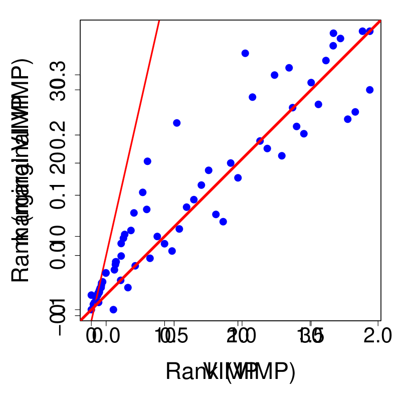
Figure 2: Differences between marginal VIMP and the VIMP index for systolic heart failure data. Left-hand figure displays the two values plotted against each other. Right-hand figure compares the ranking of variables by the two methods.

5 Robustness of VIMP to the sample size

Here we demonstrate the robustness of VIMP to the sample size. We use the systolic heart failure data as before, but this time using only a fraction of the data. We used a random 10%, 25%, 50%, and 75% of the data. This process was repeated 500 times independently. For each data set, we saved the p-values and VIMP indices for all variables. Figure 3 displays the logarithm of the p-values from the experiment (large negative values correspond to near zero p-values). Figure 4 displays the VIMP indices. What is most noticeable from Figure 4 is that VIMP indices are informative even in the extremely low sample size setting of 10%. For example, VIMP interquartile values (the lower and upper ends of the boxplot) are above zero for peak VO₂, BUN, and treadmill exercise time, showing that VIMP is able to consistently identify the top three variables even with limited data. In contrast, in Figure 3 for the low sample setting of 10%, no variable had a median log p-value below the threshold of $\log(0.05)$; showing that no variable met the 5% level of significance on average. Furthermore, even with 75% of the data, the upper end of the boxplot for exercise time is still above the threshold, showing its significance is questionable. These results demonstrate the robustness of VIMP to sample size in contrast to the p-value.

Figure 3: Logarithm of p-value as a function of fraction of sample size for systolic heart failure data (large negative values correspond to near zero p-values). Values are calculated using 500 independently subsampled data sets. Horizontal line is $\log(0.05)$, the typical threshold used to identify a significant variable.

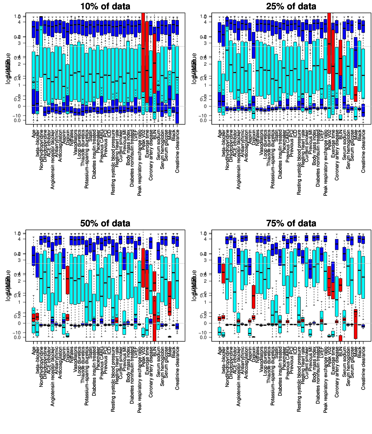
Figure 4: Subsampled data is the same as Figure 3 but where VIMP is now reported.

6 Misspecified model

For our next illustration we used simulations to demonstrate robustness of VIMP to model misspecification. For our simulation, we sampled $n=1000$ values from a Cox regression model with five variables. The first two variables are “psa” and “tumor volume” and represent variables associated with the survival outcome. The remaining three variables are noise variables with no relationship to the outcome. These are called $X_{1},X_{2},X_{3}$. The variable psa has a linear main effect, but tumor volume has both a linear and non-linear term. The true regression coefficient for psa is 0.05 and the coefficient for the linear term in tumor volume is 0.01. A censoring rate of approximately 70% was used. The log of the hazard function used in our simulation is given in the left panel of Figure 5. Mathematically, our log-hazard function assumes the following function

$$\log(h(t))=\alpha_{0}+0.05\times\text{psa}+0.01\times\text{tumor volume}+\psi(\text{tumor volume})$$

where $\psi(x)=0.04x^{2}-0.005x^{3}$ is a polyomial function with quadratic and cubic terms. The right panel of Figure 5 displays the log-hazard for the misspecified model that does not include the non-linear term for tumor volume.

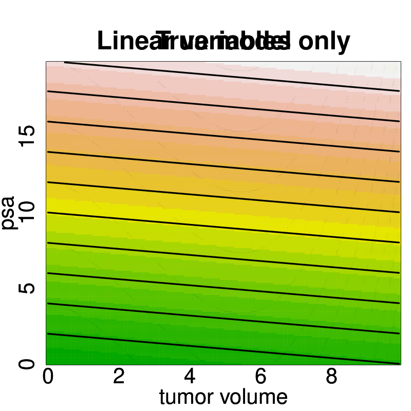
Figure 5: Log-hazard function from Cox simulation example. Left figure displays the true log-hazard function which includes the non-linear term for tumor volume. Right figure displays the log-hazard function assuming linear variables only.

We first fit a Cox regression model to the data using only linear variables as one might typically do. Following this, Algorithms 1 and 2 were applied with $B=1000$. The entire procedure was then repeated $M=1000$ times. Each of these Monte Carlo runs consisted of simulating a new data set, fitting a Cox regression model to this simulated data, and running Algorithms 1 and 2. The results are summarized in Table 4. All reported values are averaged over the $M=1000$ Monte Carlo experiments.

We first fit a Cox regression model to the data using only linear variables as one might typically do. This model was bootstrapped $B=1000$ values and VIMP and marginal VIMP calculated. This entire procedure of simulating a data set, fitting a Cox model and 1000 bootstrapped Cox models, was repeated $M=1000$ times. The results from these 1000 Monte Carlo experiments were averaged. These values are summarized in Table 4. The table shows that the p-value has no difficulty in identifying the strong effect of psa, which is correctly specified in the model. However, the p-value for tumor volume is 0.267, indicating a non-significant effect. The p-value tests whether this coefficient is zero, assuming the model is true, but the problem is that the fitted model is misspecified. The estimated Cox regression model inflates the coefficient for tumor volume in a negative direction (estimated value of -0.03, but true value is 0.01) in an attempt to compensate for the non-linear effect that was excluded from the model. This leads to the invalid p-value. In contrast, both the VIMP and marginal VIMP values for tumor volume are positive. Although these values are substantially smaller than the values for psa, VIMP is still able to identify a predictive effect size associated with tumor volume. Once again, this is possible because VIMP bases its estimation on test data and not a presumed model which can be incorrect. Also, notice that all three noise variables are correctly identified as uninformative. All have negative VIMP values.

Table 4: Results from analysis of simulated Cox regression data set. The model is misspecified by failing to include the non-linear term for tumor volume.

	$\hat{\beta}$	p-value	${\hat{\beta}_{\text{inbag}}}$	$\Delta_{\beta}$	$\Delta_{\beta}^{\!\text{marg}}$
psa	0.05	0.001	0.05	6.32	6.34
tumor volume	-0.03	0.267	-0.03	0.14	0.15
$X_{1}$	0.00	0.490	0.00	-0.25	-0.25
$X_{2}$	0.00	0.486	0.00	-0.25	-0.25
$X_{3}$	0.00	0.493	0.00	-0.27	-0.27

The overall OOB model error is 43%.

Typically, a standard analysis would end after looking at the p-values. However, a researcher with access to the entire Table 4 might be suspicious of the small positive VIMP of tumor volume and its negative coefficient value which is unexpected from previous experience. This combined with the high OOB model error (equal to 43%) should alert them to consider more sophisticated modeling. This is easily done using standard statistical methods. Here we use B-splines (Eilers and Marx, 1996) to add non-linearity to tumor volume. This expands the design matrix for the Cox regression model to include additional columns for the B-spline expansion of tumor volume. When noising up tumor volume all of these B-spline columns are noised up simultaneously (i.e. their coefficient estimates are set to zero). The extensions to Algorithms 1 and 2 are straightforward.

Table 5: Results from Cox regression simulation using a B-spline to model non-linearity in tumor volume.

	$\Delta_{\beta}$	$\Delta_{\beta}^{\!\text{marg}}$
psa	4.20	4.23
tumor volume	2.27	2.31
$X_{1}$	-0.20	-0.20
$X_{2}$	-0.20	-0.20
$X_{3}$	-0.21	-0.21

The overall OOB model error is 40%.

The results from the B-spline analysis are displayed in Table 5. As before, the entire procedure was repeated $M=1000$ times, with values averaged over the Monte Carlo runs. Notice the large values of VIMP for tumor volume. The overall model performance has also improved to 40%. Overall, results have improved substantially.

7 Discussion

It seems questionable that the p-value can continue to meet the needs of scientists. It does not provide an interpretable scientific effect size that researchers desire and it is valid only if the underlying model holds, which can often be questionable given the restrictive assumptions often used with traditional modeling. In this paper, we introduced VIMP as an alternative approach. VIMP provides an interpretable measure of effect size that is robust to model misspecification. It uses prediction error based on out-of-sample data and replaces statistical significance with predictive importance. The VIMP framework is feasible to all kinds of models including not only parametric models, such as those considered here, but also non-parametric models such as those used in machine learning approaches.

We discussed two types of VIMP measures: the VIMP index and the marginal VIMP. The scientific application will dictate which of these is more suitable. VIMP indices are appropriate in settings where variables for the model are already established and the goal is to identify the predictive effect size. For example, if several genetic markers are already identified as a genetic cause for coronary heart disease risk, VIMP can provide a rank for these and estimate the magnitude each marker plays in the prediction for the outcome. Marginal VIMP is appropriate when the goal is new scientific discovery. For instance, if a researcher is proposing to add a new genetic marker for evaluating coronary heart disease risk, marginal VIMP can yield a discovery effect size for how much the new proposed marker adds to previous risk models.

From a statistical perspective, VIMP idices are an OOB alternative to the regression coefficient p-value. However, what VIMP measures about a variable can be very flexible. It may be a linear effect, or quite easily a non-linear effect, such as modeled using B-splines. An important feature is that degrees of freedom and other messy details required with p-values when dealing with complex modeling are never an issue with VIMP. Marginal VIMP is an OOB analog to the likelihood-ratio test. In statistics, likelihood-ratio tests compare the goodness-of-fit of two models, one of which (the null model with certain variables removed) is a special case of the other (the alternative model with all variables included). Marginal VIMP compares the prediction precision of these two scenarios.

Because both VIMP and marginal VIMP are measures of predictive importance, their values are standardized to the measure of prediction performance used. This makes it possible to compare values across different data sets. For example, a 0.05 VIMP value for two different variables from two different survival datasets is comparable—both imply a 5% contribution to the concordance index. Another feature which we touched upon briefly in our B-spline example is the ability to use VIMP to measure the effect of groups of variables. In our B-spline example, the cluster of variables used were the B-spline contributions to tumor volume, and were combined together to give an overall estimate of the effect of tumor volume. One could easily extend this to calculate cluster-VIMP as a better sense of the importance of a highly correlated group of variables.

References

- Breiman et al. (1984) Breiman L., Friedman J.H., Olshen R.A., and Stone C.J. Classification and Regression Trees. Wadsworth, Belmont, California, 1984.
- Breiman (1996) Breiman, L. Out-of-bag estimation. Technical report, Statistics Dept., University of California at Berkeley, CA, 1996.
- Breiman (1996) Breiman, L. Bagging predictors. Machine learning, 24(2), 123–140, 1996.
- Breiman (2001a) Breiman, L. Statistical modeling: The two cultures (with comments and a rejoinder by the author). Statistical Science, 16(3), pp.199–231, 2001a.
- Breiman (2001b) Breiman, L. Random forests. Machine learning, 45(1), 5–32, 2001b.
- Efron (1983) Efron B. Estimating the error rate of a prediction rule: improvement on cross-validation. J. Amer. Stat. Assoc., 78:316–331, 1983.
- Efron and Tibshirani (1997) Efron B. and Tibshirani R. Improvements on cross-validation: the .632+ bootstrap method. J. Amer. Stat. Assoc., 92:548–560, 1997.
- Eilers and Marx (1996) Eilers P.H.C. and Marx B.D. Flexible smoothing with B-splines and penalties. Statistical Science, pages 89–102, 1996.
- Hsich et al. (2011) Hsich E., Gorodeski E.Z., Blackstone E.H., Ishwaran H., and Lauer M.S. Identifying important risk factors for survival in systolic heart failure patients using random survival forests. Circ. Cardiovasc. Qual. Outcomes, 4(1):39–45, 2011.
- Ishwaran et al. (2008) Ishwaran H., Kogalur U.B., Blackstone E.H., and Lauer M.S. Random survival forests. Annals of Applied Statistics, 2(3):841–860, 2008.
-
Nuzzo (2014)
Nuzzo, R. (2014),
Scientific method: statistical errors.
Nature, 506, 150–152, 2014.
www.nature.com/news/scientific-method-statistical-errors-1.14700 - Trafimow and Marks (2015) Trafimow, D. and Marks, M. Editorial. Basic and Applied Social Psychology, 37(1):1–2, 2015.
- Wasserstein and Lazar (2016) Wasserstein, R.L. and Lazar, N.A. The ASA’s statement on p-values: context, process, and purpose. The American Statistician, 70, 129–133, 2016.