Evaluating (and Improving) Estimates of the Solar Radial Magnetic Field Component from Line-of-Sight Magnetograms

Abstract

Although for many solar physics problems the desirable or meaningful boundary is the radial component of the magnetic field $B_{\rm r}$, the most readily available measurement is the component of the magnetic field along the line-of-sight to the observer, $B_{\rm los}$. As this component is only equal to the radial component where the viewing angle is exactly zero, some approximation is required to estimate $B_{\rm r}$ at all other observed locations. In this study, a common approximation known as the “$\mu$-correction”, which assumes all photospheric field to be radial, is compared to a method which invokes computing a potential field that matches the observed $B_{\rm los}$, from which the potential field radial component, $B_{\rm r}^{\rm pot}$ is recovered. We demonstrate that in regions that are truly dominated by radially-oriented field at the resolution of the data employed, the $\mu$-correction performs acceptably if not better than the potential-field approach. However, it is also shown that for any solar structure which includes horizontal fields, i.e. active regions, the potential-field method better recovers both the strength of the radial field and the location of magnetic neutral line.

1 Introduction

sec:intro

Studies of the solar photospheric magnetic field are ideally performed using the full magnetic field vector; for many scientific investigations which may not require the full vector, it is the radial component $B_{\rm r}$ which is often desired, as is derivable from vector observations. Yet observations of the full magnetic vector are significantly more difficult to obtain, from both instrumentation and data-reduction/analysis points of view, than obtaining maps of solely the line-of-sight component of the magnetic field $B_{\rm los}$. Observations consisting of the line-of-sight component can accurately approximate the radial component only along the Sun-Earth line, that is where the observing angle $\theta=0$, or $\mu=\cos(\theta)=1.0$. Away from that line, i.e. at any non-zero observing angle, the line-of-sight component deviates from the radial component. Observing solely the line-of-sight component of the solar photospheric magnetic field implies that the observing angle $\theta$ imposes an additional difficulty in interpreting the observations – it is not simply that the full strength and direction of the magnetic vector is unknown, but the contribution of these unknown quantities to the $B_{\rm los}$ signal changes with viewing angle. In other words, when $\mu=\cos(\theta)=1.0$, the line-of-sight component $B_{\rm los}$ is equal to the radial component $B_{\rm r}$. Nowhere else is this true.

A common approach to alleviate some of this “projection effect” on the inferred total field strength is to assume that the field vector is radial everywhere; then by dividing the observed $B_{\rm los}$ by $\mu$, an approximation to the radial field may be retrieved. This is the “$\mu$-correction”. Its earliest uses first supported the hypothesis of the overall radial nature of plage and polar fields, and provided a reasonable estimate of polar fields for heliospheric and coronal magnetic modeling [Svalgaard, Duvall, and Scherrer (1978), Wang and Sheeley (1992)]. However, it was evident from very early studies using longitudinal magnetographs and supporting chromospheric imaging that sunspots were composed of fields which were significantly non-radial, i.e. inclined with respect to the local normal. This geometry can lead to the notorious introduction of apparent flux imbalance and “false” magnetic polarity inversion lines (see Figure fig:projection) when the magnetic vector’s inclination relative to the line-of-sight surpasses $90^{\circ}$ while the inclination to the local vertical remains less than $90^{\circ}$ or vice versa [Chapman and Sheeley (1968), Pope and Mosher (1975), Giovanelli (1980), Jones (1985)]. Although this artifact can be cleverly used for some investigations [Sainz Dalda and Martínez Pillet (2005)] it generally poses a hindrance to interpreting the inherent solar magnetic structure present.

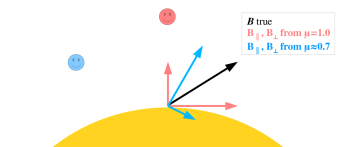
Figure 1.: Geometry of projection effects when observing a photospheric magnetic field vector (black) in the image plane, from two different perspectives. Of note regarding the inferred polarity is that the $B_{\rm los}$ component (pointed toward/away from the observer) changes sign between the $\mu=1.0$ and $\mu=0.7$ viewing angles. fig:projection

The inaccuracies which arise from using $B_{\rm los}$ are generally assumed to be negligible when the observing angle $\theta$ is less than $30^{\circ}$; if the field is actually radial, the correction is only a $\approx 13$% error, and introduced false neutral lines generally appear only in the super-penumbral areas. Yet this is a strong assumption, and one known to be inaccurate for many solar magnetic structures. The estimates of polar radial field strength are especially crucial for global coronal field modeling and solar wind estimations [Riley et al. (2006), Riley et al. (2014)], but these measurements are exceedingly difficult [Tsuneta et al. (2008), Ito et al. (2010), Petrie (2015)].

The gains afforded by using the full magnetic vector include the ability to better estimate the $B_{\rm r}$ component by way of a coordinate transform of the azimuthally-disambiguated inverted Stokes vectors [Gary and Hagyard (1990)]. However, although there are instruments now which routinely provide full-disk vector magnetic field data (such as SOLIS, solis; HMI hmi_pipe), the line-of-sight component $B_{\rm los}$ remains the least noisy, easiest measurement of basic solar magnetic field properties.

We present here a method of retrieving a different, and in the case of sunspots, demonstrably better, estimate of the radial field boundary, $B_{\rm r}^{\rm pot}$, the radial component of a potential field which is constructed from $B_{\rm los}$ so as to match to the observed line-of-sight component. This approach was originally described by Sakurai1982 and Alissandrakis1981, but is rarely used in the literature. We demonstrate here its implementation, including in spherical geometry for full-disk data. The method is described in section sec:method, the data used are described in section sec:data, and both the planar and spherical results for $B_{\rm r}^{\rm pot}$ are evaluated quantitatively for active-region and solar polar areas in section sec:arcomps and sec:fluxcomps. In section sec:rcomps we reflect specifically on the different approximations in the context of “false polarity-inversion lines” artifacts, and in section sec:successNfailure we investigate the reasons behind both regions of success and areas of failure.

2 Method

sec:method

Approaches to computing the potential field which matches the observed line-of-sight component are outlined here for two geometries, with details given in Appendices app:method_planar and app:method_spherical. When one is focused on a limited part of the Sun such that curvature effects are minimal, a planar approach can be used to approximate the radial field (section sec:method_planar, appendix app:method_planar). The planar approach is fast, and reasonably robust for active-region sized patches (section sec:arcomps). When the desired radial-field boundary is the full disk, or covers an extended area of the disk, such as the polar area, then the spherical extension of the method is the most appropriate (section sec:method_spherical, appendix app:method_spherical); however, depending on the image size of the input, calculating the radial field in this way can be quite slow.

2.1 Method: Planar Approximation

sec:method_planar

The line-of-sight component is observed on an image-coordinate planar grid. We avoid having to interpolate to a regular heliographic grid by performing the analysis using a uniform grid in image coordinates, $(\xi,\eta)$. Restricting the volume of interest to $0<\xi<L_{x}$, $0<\eta<L_{y}$ and $z\geq 0$, and neglecting curvature across the field of view, the potential field can be written in terms of a scalar potential $\mbox{\boldmath$B$}^{\rm pot}=\mbox{\boldmath$\nabla$}\Phi$, with the scalar potential given by

$$\Phi(\xi,\eta,z) = \sum_{m,n}A_{mn}e^{[2\pi im\xi/L_{x}+2\pi in\eta/L_{y}-\kappa_{mn}z]}+A_{0}z,$$ (1)

where $z$ is the vertical distance above the solar surface. The value of $\kappa_{mn}$ is determined by $\mbox{\boldmath$\nabla$}^{2}\Phi=0$, namely

$$\kappa_{mn}^{2} = (2\pi)^{2}\bigg{[}(c_{11}^{2}+c_{12}^{2})\bigg{(}{m\over L_{x}}\bigg{)}^{2}+2(c_{11}c_{21}+c_{12}c_{22})\bigg{(}{m\over L_{x}}\bigg{)}\bigg{(}{n\over L_{y}}\bigg{)}$$ (2)

$$\qquad+(c_{21}^{2}+c_{22}^{2})\bigg{(}{n\over L_{y}}\bigg{)}^{2}\bigg{]},$$

where $c_{ij}$ are the coordinate transformation coefficients given in garyhagyard90, and choose $\kappa_{mn}>0$ so the field stays finite at large heights. The values of the coefficients $A_{mn}$ are determined by requiring that the observed line-of-sight component of the field matches the line-of-sight component of the potential field, which results in

$${\tt FFT}(B^{l}) = L_{x}L_{y}A_{jk}\bigg{[}{2\pi ij\over L_{x}}(c_{11}a_{13}+c_{12}a_{23})+{2\pi ik\over L_{y}}(c_{21}a_{13}+c_{22}a_{23})-\kappa_{jk}a_{33}\bigg{]}$$ (3)

$$\quad+L_{x}L_{y}a_{33}A_{0}\delta_{0j}\delta_{0k}.$$

where $a_{ij}$ are the elements of the field components transformation matrix given in garyhagyard90, and ${\tt FFT}(B^{l})$ denotes taking the Fourier Transform of $B^{l}$. The value of $A_{0}$ is determined by the net line-of-sight flux through the field of view.

Placing the tangent point at the center of the presented field of view (corresponding to evaluating the coordinate transformation coefficients and the field components transformation matrix at the longitude and latitude of the center of the field of view) is the default, producing a boundary labeled $B_{\rm z}^{\rm pot,center}$. The resulting radial component estimation is least accurate near the edges, as expected, and as such we also present $B_{\rm r}^{\rm pot,all}$, for which the tangent point is placed at each pixel presented, the field calculated, and only that pixel’s resulting radial field (for which it acted as the tangent point) is included.

2.2 Method: Spherical Case

sec:method_spherical

The potential field in a semi-infinite volume $r\geq R$ can be written in terms of a scalar potential $\mbox{\boldmath$B$}^{\rm pot}=-\mbox{\boldmath$\nabla$}\Psi$, given by

$$\Psi = R\sum_{n=1}^{\infty}\sum_{m=0}^{n}\bigg{(}{R\over r}\bigg{)}^{n+1}(g_{n}^{m}\cos m\phi+h_{n}^{m}\sin m\phi)P_{n}^{m}(\mu),$$ (4)

where $\mu=\cos\theta$. Defining the coordinate system such that the line of sight direction corresponds to the polar axis of the expansion results in particularly simple expressions for the coefficients $g_{n}^{m}$, $h_{n}^{m}$ [Rudenko (2001)]. However, because observations are only available for the near side of the Sun, it is necessary to make an assumption about the far side of the Sun. The resulting potential field at the surface $r=R$ is not sensitive to this assumption except close to the limb, so for convenience, let $B_{l}(R,\pi-\theta,\phi)=B_{l}(R,\theta,\phi)$, where the front side of the Sun is assumed to lie in the range $0<\theta<\pi/2$.

With these conventions, the coefficients are determined from

$$g_{n}^{m} = \cases{{(2n+3)(n-m)!\over 2\pi(n+m+1)!}\int_{0}^{2\pi}d\phi\,\cos m\phi\int_{0}^{1}d\mu\,P_{n+1}^{m}(\mu)B_{l}(R,\mu,\phi)&$n+m$ odd\cr 0&$n+m$ even\cr}$$ (5)

and

$$h_{n}^{m} = \cases{{(2n+3)(n-m)!\over 2\pi(n+m+1)!}\int_{0}^{2\pi}d\phi\,\sin m\phi\int_{0}^{1}d\mu\,P_{n+1}^{m}(\mu)B_{l}(R,\mu,\phi)&$n+m$ odd\cr 0&$n+m$ even\cr}$$ (6)

and the radial component of the field is given by

$$B_{r} = -{\partial\Psi\over\partial r}=\sum_{n=1}^{\infty}\sum_{m=0}^{n}(n+1)\bigg{(}{R\over r}\bigg{)}^{n+2}(g_{n}^{m}\cos m\phi+h_{n}^{m}\sin m\phi)P_{n}^{m}(\mu).$$ (7)

When evaluated at $r=R$, this produces a full-disk radial field boundary designated $B_{\rm r}^{\rm pot,sph}$ from which extracted HARPs and polar sub-regions are analyzed below. Our implementation of this approach uses the Fortran 95 SHTOOLS library [Wieczorek et al. (2016)] for computing the associated Legendre functions. The routines in this library are considered accurate up to degrees of $n\approx 2800$. For the results presented here, a value of $n=2048$ was used, corresponding to a spatial resolution of about 2 Mm.

3 Data

sec:data

For this study we use solely the vector magnetic field observations from the Solar Dynamics Observatory [Pesnell (2008)] Helioseismic and Magnetic Imager [Scherrer et al. (2012), Hoeksema et al. (2014)]. Two sets of data were constructed: a full-disk test and a set of HMI Active Region Patches (“HARPs”; hmi_pipe, hmi_invert, hmi_sharps) over 5 years. For both, in order to keep comparisons as informative as possible, we construct line-of-sight component data from the vector data by transforming the magnetic vector components into a $B_{\rm los}$ map: $B_{\rm los}=B\cos(\xi)$ where $\xi$ is the inclination of the vector field in the observed plane of the sky coordinate system, as returned from the inversion.

The full-disk data target is 2011.03.06_15:48:00_TAI; this date was chosen due to its extreme B0 angle such that the south pole of the Sun is visible, the variety of active regions visible at low $\mu=\cos(\theta)$ observing angle (away from disk center), and the presence of a northern extension of remnant active-region plage. The hmi.ME_720s_fd10 full-disk series was used; data are available through the JSOC lookdata tool. Because the weaker fields do not generally have their inherent $180^{\circ}$ ambiguity resolved in that series and we will be evaluating the $B_{\rm r}^{\rm pot}$ method in poleward areas of weaker field, two customizing steps were taken. First, a custom noise mask was generated ($\textsc{ambthrsh}=0$, rather than the default value of 50). Second a custom disambiguation was performed using the cooling parameters: $\textsc{ambtfctr}=0.998$, $\textsc{ambneq}=200$, $\textsc{ambngrow}=2$, $\textsc{ambntx}=\textsc{ambnty}=48$ [Hoeksema et al. (2014), Barnes et al. (2017)]; compared to the default HMI pipeline implementation, these parameters provide smaller tiles over which the potential field is computed to estimate $d{\mbox{\boldmath$B$}}/d{\rm z}$, a smaller “buffer” of noisy pixels around well-determined pixels, and slower cooling for the simulated annealing optimization. Disambiguation results were generated for 10 random number seeds. Pixels used for the comparisons shown herein are only those for which both the resulting equivalent of the conf_disambig segment is $\geq$60 and the results from all 10 random number seeds agreed, as well. This requirement translates to 75.3% of the pixels with $\textsc{conf\_disambig}\geq 60$ and 88.8% of the pixels with $\textsc{conf\_disambig}=90$ being included. In the case of the present data, there is a 0.2% chance that the disambiguation solution used results by chance, even in the weak areas (including the poles).

From this full disk magnetogram the nine identified HMI Active Region Patch (“HARP”) areas are extracted using the keywords harpnum, crpix1, crpix2, crsize1, crsize2 from the hmi.Mharp_720s series. Two polar regions were also extracted: a “Northern plage area”, which is an extended remnant field and a “South Pole Region” that encompasses the entire visible polar area. A context image is shown in Figure fig:harps, and summary information about each sub-area is given in Table table:harps, including the WCS coordinates for the two non-HARP regions for reproducibility. Also in Table table:harps are summary data for an additional 22 sub-areas, each $256^{2}$ pixels in size centered along the midpoints in $x,~{}y$ on the image at a variety of $\mu=\cos{\theta}$ positions.

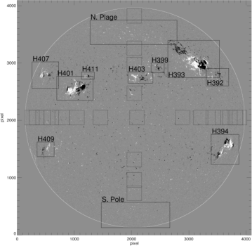
Figure 2.: Full-disk image of the line-of-sight component of the solar photospheric magnetic field on 2011.03.06 at 15:48:00_TAI, scaled to $\pm 200$G. The solar limb is indicated as are the HMI Active Region Patches labeled with their “HARP number”, and the additional two polar areas used for this analysis. Additional small patches of quiet-Sun, distributed in $\mu=\cos{\theta}$ are indicated as grey boxes, occasionally overlapping. Solar north is up, west to the right, positive/negative directed field is shown as white/black respectively.fig:harps

Table 1.: Extracted Area Descriptions

I.D.	HARP	NOAA	Locale	$\mu=\cos(\theta)$	Description
	No.	AR No.
H392	392	11163	N22 W54	0.54	small plage
H393	393	11164	N32 W39	0.65	large complex active region
H394	394	11165	S17 W59	0.49	small active region
H399	399	N/A	N27 W13	0.87	small plage
H401	401	11166	N15 E34	0.79	simple active region
H403	403	11167	N21 W03	0.93	bipolar plage
H407	407	11169	N23 E62	0.43	small active region
H409	409	N/A	S17 E58	0.51	small plage
H411	411	N/A	N22 E27	0.92	small spot
N.Plage	N/A	N/A	N51 E01	0.63	north remnant plage
					crpix1=1304 crpix2=344
					crsize1=1516 crsize2=428
S.Pole	N/A	N/A	S60 E01	0.51	south polar area
					crpix1=1199 crpix2=3527
					crsize1=1427 crsize2=440
QS_E_350	N/A	N/A	N00 E70	0.35	crpix1=3709 crpix2=1921
QS_E_450	N/A	N/A	N00 E63	0.45	crpix1=3625 crpix2=1921
QS_E_550	N/A	N/A	N00 E57	0.55	crpix1=3514 crpix2=1921
QS_E_650	N/A	N/A	N00 E49	0.65	crpix1=3370 crpix2=1921
QS_E_750	N/A	N/A	N00 E41	0.35	crpix1=3181 crpix2=1921
QS_E_850	N/A	N/A	N00 E32	0.85	crpix1=2923 crpix2=1921
QS_E_950	N/A	N/A	N00 E18	0.95	crpix1=2511 crpix2=1921
QS_W_1000	N/A	N/A	N00 W01	1.00	crpix1=1874 crpix2=1921
QS_W_900	N/A	N/A	N00 W26	0.90	crpix1=1076 crpix2=1921
QS_W_800	N/A	N/A	N00 W37	0.80	crpix1=761 crpix2=1921
QS_W_700	N/A	N/A	N00 W46	0.70	crpix1=542 crpix2=1921
QS_W_600	N/A	N/A	N00 W53	0.60	crpix1=377 crpix2=1921
QS_W_500	N/A	N/A	N00 W60	0.50	crpix1=251 crpix2=1921
QS_W_400	N/A	N/A	N00 W66	0.40	crpix1=154 crpix2=1921
QS_W_300	N/A	N/A	N00 W72	0.30	crpix1=82 crpix2=1921
QS_N_375	N/A	N/A	N68 E01	0.375	crpix1=1921 crpix2=143
QS_N_775	N/A	N/A	N39 E00	0.775	crpix1=1921 crpix2=708
QS_N_875	N/A	N/A	N29 E00	0.875	crpix1=1921 crpix2=992
QS_N_975	N/A	N/A	N13 E00	0.975	crpix1=1921 crpix2=1495
QS_S_925	N/A	N/A	S22 E00	0.925	crpix1=1921 crpix2=2650
QS_S_825	N/A	N/A	S34 E00	0.825	crpix1=1921 crpix2=3005
QS_S_725	N/A	N/A	S44 E00	0.725	crpix1=1921 crpix2=3242
table:harps

Throughout this study, we differentiate between when planar approximations are invoked and when curvature is accounted for by referring to “$B_{\rm z}$” and “$B_{\rm r}$”, respectively. The potential-field approximation is performed three ways, as described in section sec:method, above: using a planar approximation from the center-point coordinates $B_{\rm z}^{\rm pot,center}$ of each HARP or extracted sub-region, using a planar approximation with each point of the extracted region used as the center point $B_{\rm r}^{\rm pot,all}$, and using the spherical full-disk approach $B_{\rm r}^{\rm pot,sph}$. In addition, we calculate two common $\mu$-correction approximations for each sub-region: the center point value of $\mu=\cos(\theta)$ used as a tangent point to obtain $B_{\rm z}^{\mu}=B_{\rm los}/\mu$, and secondly each pixel’s $\mu$ value is calculated and applied independently, for $B_{\rm r}^{\mu(s)}=B_{\rm los}/\mu(s)$ where $(s)$ is the spatial location of the pixel.

The second set of data consists of a subset of all HARPs selected over 5.5 years, selected so as to generally not repeat sampling any particular HARP: on days ending with ’5’ (5th, 15th, and 25th) of all months 2010.05 – 2015.06, the first ‘good’ (quality flag is 0) HARP set at :48 past each hour on/after 15:48 was used. HARPs which were defined but for which there were no active pixels are skipped. The result is 1,819 extracted HARPs without regard for size, complexity, or location on the disk. Effectively the hmi.Bharp_720s series was used, including the standard pipeline disambiguation. NWRA’s database initially began construction prior to the pipeline disambiguation being performed for earlier parts of the mission, thus for some of the data base, the hmi.ME_720s_fd10 data were used, the HARP regions extracted and the disambiguation performed in-house, matching the implementation performed in the HMI pipeline. All analysis is performed up to $80^{\circ}$ from disk center, and only points with significant signal/noise in the relevant components ($S/N>3$ relative to the returned uncertainties from the inversion, and propagated accordingly) are included in the analyses. For this larger dataset, all calculations are done with a planar approximation. The “answer” is $B_{\rm z}$, and the boundary estimates calculated are: $B_{\rm z}^{\mu}=B_{\rm los}/\mu$, $B_{\rm r}^{\mu(s)}=B_{\rm los}/\mu(s)$ (which imparts a spherical accounting due to the variation of $\mu$ over the field of view), and $B_{\rm z}^{\rm pot,center}$. $B_{\rm r}^{\rm pot,all}$ and $B_{\rm r}^{\rm pot,sph}$ are computationally possible but extremely slow, and are not employed for this second dataset.

4 Results

For the results presented here, the “golden standard” is taken to be the radial or normal field as computed from the vector data, and to this quantity we compare results of different approximations of the boundary. We do caution that $B_{\rm r}$ data do include the observed $B_{\rm trans}$ component, which is inherently noisier than the $B_{\rm los}$ component. Additionally we stress that the comparisons are performed against a particular instrument’s retrieval of the photospheric magnetic field vector, which may not reflect the true Sun as per influences in polarimetric sensitivity, spectral finesse, spatial resolution, etc.

4.1 Field Strength Comparisons

sec:arcomps

To demonstrate the general resulting trends for each of the radial field approximations, we first present density-histograms of the inferred radial field strengths for two representative sub-regions, NOAA AR 11164 (HARP #393, Figure fig:scat393) and the south pole region (Figure fig:scatspole). Throughout, we do not indicate the errors for clarity; a 10% uncertainty in field strength is a fair approximation overall, and a detailed analysis beyond that level is not informative here.

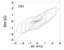
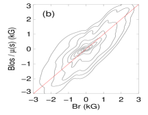
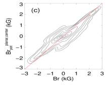
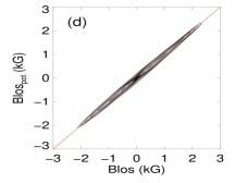
Figure 3.: (a)–(c) Non-parametric density estimates comparing the distribution of the radial field from the vector field data $B_{\rm r}$ (x-axis) to the inferred radial field strength estimates using representatives of the different models discussed in the text (y-axis). Shown here are distributions from NOAA AR 11164 (H393). Contour levels are equal in log (probability) ranging from [$10^{-3}-10^{2}$], with $x=y$ line included for reference. The comparisons are for $B_{\rm r}$ against (a) $B_{\rm los}$ (b) $B_{\rm los}/\mu(s)$, (c) $B_{\rm z}$ potential, planar, center-point pivot Panel (d) shows, in summary, that the $\mu$-corrected estimates generally show less bias compared to the $B_{\rm los}$ fields, but still have a large random error. The potential field corrected fields show larger differences for weak field strengths, but less random error. In (d) the scatter plot is between the $B_{\rm los}$ calculated from the inversion, and the recovered $B_{\rm los}$ calculated from the spherical potential vector (Sect. app:method_spherical). While the boundary is thus fairly well recovered, the disagreement beyond machine-precision differences is due to the spherical calculation not being performed with high enough degree to remove all small-scale “ringing”. fig:scat393

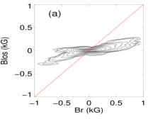
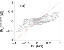
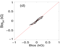
Figure 4.: Same as Figure fig:scat393, but for the south pole area shown in Figure fig:harps. These panels show, in summary, that the $\mu$-corrected estimates for the south polar area show distinct spurs with incorrect polarity while the potential field estimates have large biases. fig:scatspole

For both HARP H393 (NOAA AR 11164) and the south pole area, the initial comparison of $B_{\rm los}$ to $B_{\rm r}$ (panel (a) in Figures fig:scat393, fig:scatspole) shows the expected signature of underestimated field strengths overall. Note that for both regions, but especially for the the south pole, there is a strong underestimation of the radial field strength across magnitudes.

The $B_{\rm r}^{\mu(s)}$ correction (panel (b) in Figures fig:scat393, fig:scatspole; the $B_{\rm z}^{\mu}$ plot is almost identical and not shown here) shows improvement by eye for both regions, with distributions systematically deviating less from the $x=y$ line. However, in the case of the H393 corrections, the stronger-field strengths are often over-corrected, and the opposite-polarity erroneous pixels are exacerbated in their error. This trend is also true for the south pole area: both an improvement (especially for stronger-field points) and the appearance of a distinct erroneous opposite-polarity spur in the $B_{\rm r}^{\mu(s)}$ results.

In the next panel (panel (c) in Figures fig:scat393, fig:scatspole), a representative potential-field option, $B_{\rm z}^{\rm pot,center}$, is shown with regards to $B_{\rm r}$ (again, $B_{\rm r}^{\rm pot,sph}$ and $B_{\rm r}^{\rm pot,all}$ plots look essentially identical); the weaker field strengths appear to be less-well corrected than the $B_{\rm r}^{\mu(s)}$ approximation, although the strong-field approximations for the sunspots in H393 are significantly better than the $B_{\rm r}^{\mu(s)}$ correction. There appears to be a small number of points for which the opposite polarity is retained but overall the stronger field points (generally $\geq 1000$ G) lie close to the $x=y$ line. There are still significant deviations from the $B_{\rm r}$ field; this is expected at some level since a potential-field model is being imposed, and it cannot be expected that the solar magnetic fields are in fact potential. Additionally, while a non-linear force-free field model may better represent the true field [Livshits et al. (2015)], there is insufficient information in the $B_{\rm los}$ boundary with which to construct such a model. For the south pole region, the strong-field areas are less well corrected than was seen in the $B_{\rm r}^{\mu(s)}$ plot (Figure fig:scatspole, panels c, b respectively), but the distinct incorrect-polarity spur visible for $B_{\rm r}^{\mu(s)}$ is less pronounced in the potential-field-based estimate.

For completeness, and as a check of the algorithm, the $B_{\rm los}$ directly attained from the inversion as $B_{\rm los}=|\mbox{\boldmath$B$}|\cos(\xi)$ where $\xi$ is the inclination of the field vector to the line of sight (and which constitutes the input to the potential field calculation), is compared with the $B_{\rm los}^{\rm pot}$ derived from the vector field components from the derived potential field (panel (d) in Figures fig:scat393, fig:scatspole). These $B_{\rm los}$ boundaries match well, indicating that there is little if any systematic bias presented by the potential field calculation when recovering the input boundary. The recovery is not, however, within machine precision due to the lower than optimal degree to which the spherical potential field is computed; to reproduce the boundary to machine precision is computationally untenable with this algorithm.

The two examples shown in Figures fig:scat393, fig:scatspole represent the two extremes of solar magnetic features to which these approximations would be applied: the south polar region (expected to sample small, primarily radially-directed concentrations of field) and a large active region with both plage and sunspots. The distributions of the other sub-regions appear as hybrids when examined in the same manner, having sometimes stronger fields for which the $\mu$-corrections approaches perform the best (e.g., the northern plage area), or having sunspot areas for which there is an incorrect-polarity spur present in the distributions that is exacerbated by some amount in the $\mu$-corrections and mitigated by some amount with the potential-field calculations.

To summarize the performance of these approaches, quantitative metrics of the comparisons between $B_{\rm r}$ and the different estimations for the sub-regions on 2011.03.06 are presented graphically in Figures fig:stats_all, fig:stats_strong, fig:stats_weak, for all HARP-based sub-regions plus the north and south targets considered, and in Figure fig:stats_qs for the small quiet-sun extractions. The metrics considered are: the linear correlation coefficient, the fitted linear regression slope and constant, a mean signed error, a root-mean-square error, and the percentage of pixels that show the incorrect sign relative to $B_{\rm r}$. All well-measured points within each sub-region are considered in Figure fig:stats_all (see section  sec:data), and in Figures fig:stats_strong, fig:stats_weak the results are separated between strong and weaker field areas as well.

What is clear is that there is not, in fact, a single best approach. In some cases, e.g. for H394 and H407, by almost all measures the $B_{\rm r}^{\rm pot,sph}$ and $B_{\rm z}^{\rm pot,center}$ approaches improve upon $B_{\rm los}$ and the $\mu$-correction methods. The latter generally show less bias compared to the uncorrected $B_{\rm los}$ field, but still have a large random error. The potential-field based estimates show larger differences for weak field strengths, but less random error. Comparing the weak- and strong-field results, it is clear that the small correlations and regression slopes in the former are due to the abundance of weak-field points and their low response to the corrections (see Fig. fig:scat393 vs. fig:scatspole). However, there is a general trend that plage- or weaker-field dominated areas, including the two polar areas, are better served (under this analysis) by the $\mu$-correction methods, notwithstanding the polarity-sign errors. This is confirmed as a general trend by the quiet-sun areas (Figure fig:stats_qs) whose underlying structures – like the polar area and plage areas – are likely predominantly radial in HMI data. In contrast, when the sub-areas include or are dominated by sunspots, (e.g., H393, H394, H401, H407), the $B_{\rm r}^{\rm pot,sph}$ and $B_{\rm z}^{\rm pot,center}$ perform the best by these metrics. The reasons behind this “mixed” message of success is explored further, below.

Regarding the quiet-sun patches, these are sampled in order to test the dependence of the approximations to $\mu$ only, without the complications of different underlying structure: we assume these comprise similar samples of small primarily radial magnetic structures. Indeed in Figure fig:stats_qs, definitive trends with $\mu$ are seen. All models improve with increasing $\mu$ by these metrics, and there is no obvious difference in trends between quadrants (East, North, etc.). There are outliers, which are likely due to inherent underlying structure. The $\mu$-correction methods generally better serve these areas, by a small degree in some measures, than the potential-field methods. However, all regions except those with $\mu\approx 1.0$ have a higher percentage of points with the incorrect sign than all of the HARP regions, except for the South Polar area.

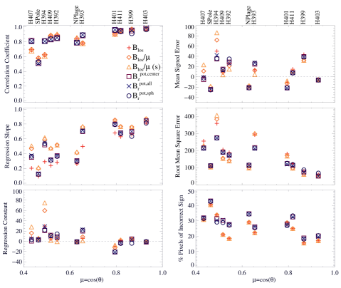
Figure 5.: Metrics to evaluate the performance of radial-field approximations when compared to $B_{\rm r}$, for the cut-out areas highlighted in Figure fig:harps. Top to Bottom, Left: the linear correlation coefficient, the slope of the linear regression line, the constant (offset) for that fit, and Right: the mean error, the root mean square error, the percent of pixels which are of the incorrect sign. In shades of orange, $+$: $B_{\rm los}$, $\Diamond$: $B_{\rm z}^{\mu}$, $\triangle$: $B_{\rm r}^{\mu(s)}$; in shades of purple, $\Box$: $B_{\rm z}^{\rm pot,center}$, $X$: $B_{\rm r}^{\rm pot,all}$, $\bigcirc$: $B_{\rm r}^{\rm pot,sph}$. These metrics demonstrate some trends (less spread between methods with increasing $\mu$) but also a mix of results between regions, $\mu$ and methods, indicating no single best approach. fig:stats˙all

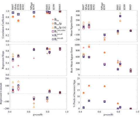
Figure 6.: Same as Figure fig:stats_all but only for points with total field strengths $|\mbox{\boldmath$B$}|>1000$G (note the different scales from prior figures for some metrics). As some of the sub-regions do not meet the additional restriction of having a minimum of 100 such points, they are not included in this plot. Note that compared with Fig. fig:stats_all, there are in some cases stronger distinctions between the method categories, and much weaker relationships with $\mu=\cos(\theta)$ for some metrics.fig:stats˙strong

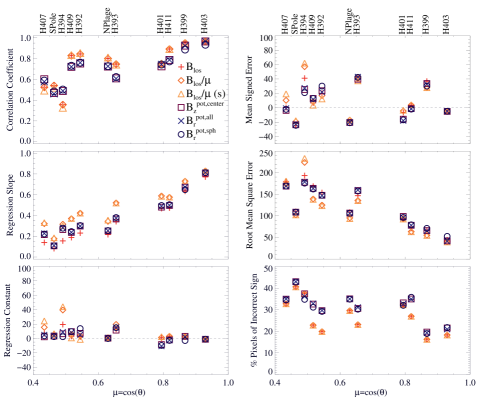
Figure 7.: Same as Figure fig:stats_all but only for points with $B_{\rm h}<500$G and $|B_{\rm r}|<500$G (note the different scales for some metrics). Some metrics once again show strong relationship with $\mu$, and again there presents less of a strong trend between the method categories.fig:stats˙weak

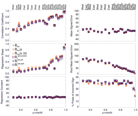
Figure 8.: Same as Figure fig:stats_all but for the small quiet-sun extractions at a thorough sampling of $\mu$. Top label indicates the quadrant from which the extraction originated.fig:stats˙qs

4.2 Total Flux Comparisons

sec:fluxcomps

The second test is the total magnetic flux of the sub-regions, where the estimates of the magnetic flux are computed as $\sum|{\rm B}_{\rm bndry}|d{\rm A}$ over the acceptable pixels, $dA$ is the area in Mm² of each pixel (thus imparting some spherical accounting for the flux which otherwise uses a planar approximation), and ${\rm B}_{\rm bndry}=B_{\rm los},~{}B_{\rm z}^{\mu},~{}B_{\rm z}^{\rm pot,center}$ or similar as indicated. The results are summarized in Figure fig:fluxes, both for all well-measured pixels and then for only strong-field (sunspot) pixels. The results for the regions extracted from the full-disk data are considered first.

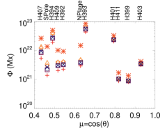
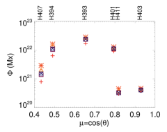
Figure 9.: A comparison of inferred total magnetic flux $\Phi=\sum|{\rm B}_{\rm bndry}|dA$ for each sub-region, as a function of the observing angle, using different radial-field approximations for the $B_{\rm r}$ boundary; for all, $dA$ is the area in Mm² of each pixel (thus imparting some spherical accounting for calculations which might otherwise use a planar approximation). Left: all points in each sub-region, Right: only those points with total field strengths over 1000 G (which removes some sub-regions from consideration). For both, the symbols and colors follow Fig. fig:stats_all with the addition of $\ast$: $B_{\rm r}$ (red). fig:fluxes

Overall, the total flux estimate using $\Phi(B_{\rm r})$ is always the largest, that using $\Phi(B_{\rm los})$ is always the smallest, with other approximations in varying order between. As demonstrated in section sec:arcomps the behaviors can be quite mixed between strong-field, sunspot areas and plage areas, making the summations over the entire sub-regions (for the total flux) difficult to interpret. What is also clear is that the degree of underestimation of the $B_{\rm los}$-based flux $\Phi(B_{\rm los})$ is a function of $\mu$, and the flux from the $B_{\rm z}^{\mu}$ boundaries do well overall at recovering the $\Phi(B_{\rm r})$ for the same data. The fluxes based on potential-field based boundaries also do not completely recover $\Phi(B_{\rm r})$, even when the area under consideration is restricted to the sunspots. The different implementations of each method do not vary significantly between each other.

Further, a close examination of Figure fig:fluxes as compared to Figure fig:scat393 shows something slightly confusing: while in Figure fig:scat393 there are indeed regions of the distribution where $|B_{\rm los}|>|B_{\rm r}|$ and certainly $|B_{\rm los}|/\mu>|B_{\rm los}|$, in Figure fig:fluxes $\Phi(B_{\rm r})>\Phi(B_{\rm los})$ and indeed $\Phi(B_{\rm r})>\Phi(B_{\rm r}^{\mu(s)})$ always. The differences decrease with increasing $\mu$ as noted above. But with a non-trivial number of points having $|B_{\rm los}|>|B_{\rm r}|$, why is the total flux consistently larger when computed using $B_{\rm r}$? The answer is that $B_{\rm r}$ includes the higher-noise component $B_{\rm trans}$, whereas any estimation using $B_{\rm los}$ does not include that higher-noise component. The impact is much larger in weak-signal areas which dominate the summation for total flux when all points are used (Figure fig:fluxes, left) and the impact is less when only strong-field points are included (Figure fig:fluxes, right). This impact of photon noise on $B_{\rm trans}$ and its particular influence on the calculation of $\Phi(B_{\rm r})$ vs. $\Phi(B_{\rm los})$ is confirmed using model data with varying amount of photon noise [Leka et al. (2009)]. As such, while in this context we consider $B_{\rm r}$ the “answer”, it is clear that it instead represents solely an observed estimate against which we compare other estimates, and is likely to be an overestimate of the true flux.

The larger HARP database is used next to examine the $\Phi({\rm B}_{\rm bndry})$ differences for a large number of extracted regions (Figure fig:fluxes_lots). In this plot, the general underestimation of $\Phi(B_{\rm r})$ by $\Phi(B_{\rm los})$ is present as expected, and varies with $\mu=\cos(\theta)$; $\Phi(B_{\rm z}^{\rm pot,center})$ also underestimates the flux relative to $\Phi(B_{\rm r})$ although not as severely, and the consistently larger $\Phi(B_{\rm r})$ is now understood, from the comments above regarding the inherent influence of noise. $\Phi(B_{\rm r}^{\mu(s)})$ is actually closer to $\Phi(B_{\rm r})$ for much of the range in observing angle, however it is also capable of overestimating the total flux, from relatively modest through large observing angles; this is a property not generally seen when using the $B_{\rm z}^{\rm pot,center}$ boundary. As such, using $\Phi(B_{\rm los})$ results in the largest systematic error, while $\Phi(B_{\rm r}^{\mu(s)})$ results in the smallest systematic error, with $\Phi(B_{\rm z}^{\rm pot,center})$ showing an intermediate systematic error relative to $\Phi(B_{\rm r})$. For the random error, the converse order holds, with $\Phi(B_{\rm r}^{\mu(s)})$ resulting in the largest random error, $\Phi(B_{\rm los})$ the smallest, with the $\Phi(B_{\rm z}^{\rm pot,center})$ random error comparable to $\Phi(B_{\rm los})$.

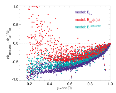
Figure 10.: Scatterplot of the differences in total flux when computed using $B_{\rm los}$, $B_{\rm r}^{\mu(s)}$, and $B_{\rm z}^{\rm pot,center}$ as indicated, as a percentage difference from the total flux computed using $B_{\rm r}$ (capped at 100% difference), as a function of observing angle $\mu=\cos(\theta)$ (limited to $\theta\leq 80^{\circ}$ from disk center). fig:fluxes˙lots

4.3 Magnetic Polarity Inversion Lines

sec:rcomps

The introduced apparent magnetic polarity changes at the edges of sunspots were very early signatures that inclined structures are prevalent in active regions. For many solar physics investigations, however, the location of, and character of the magnetic field nearby the magnetic polarity inversion line (PIL) is central to the analysis. In particular, what is often of interest are magnetic PILs with locally strong gradients in the spatial distribution of the normal field, as an indication of localized very strong electric currents which are associated with subsequent solar flare productivity [Schrijver (2007)]. Incorrect neutral lines introduced by projection may mis-identify limb-ward penumbral areas as being strong-gradient regions of interest.

Figure fig:H393rcomp shows images of the observed $B_{\rm r}$ field, then the analogous estimates from $B_{\rm los}$, $B_{\rm z}^{\mu}$ and $B_{\rm z}^{\rm pot,center}$ for H393 in detail; this sunspot group is fairly large, complex, and quite close to the limb. In particular, areas of strong-gradient neutral lines are highlighted. One can see that the location of the implied magnetic neutral line does not change at all when simply the $B_{\rm z}^{\mu}$ correction is applied to the $B_{\rm los}$ boundary, as expected from a simple scaling factor, but the highlighted areas do change because the magnitude of the gradient increases. The $B_{\rm z}^{\rm pot,center}$ boundary better replicates the $B_{\rm r}$ boundary, almost completely removing the introduced polarity lines on the limb-ward sides of the sunspots. However, it is not perfect: there is a slight decrease in the magnitude of field in the negative-polarity plage area which extends toward the north/east of the active region. This is in part due to a planar approximation being invoked, but also due to the introduction of inclined fields by the potential field model where the underlying field inferred by HMI is predominantly vertical (see section sec:successNfailure).

The recovery of a more-appropriate PIL in or near sunspots with polarity errors in weaker fields was seen earlier in the analysis of the “% Points of Incorrect Sign” in Figs. fig:stats_all–fig:stats_weak. The strong-field regions showed a significant decrease in incorrect-polarity fields when a potential-field-based boundary was used relative to the $\mu$ correction boundaries, but in the weak field areas the results were mixed, leading to a similarly mixed result when all pixels were included.

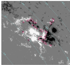
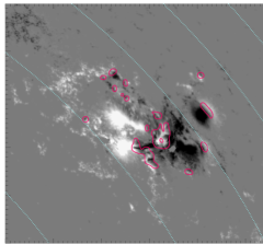
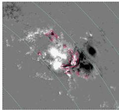
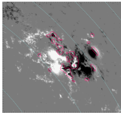
Figure 11.: Images of the boundary magnetic field for NOAA AR 11164 (a sub-area of HARP 393; c.f. Figure fig:harps), scaled to $\pm 1$kG, positive/negative (white/black). The inferred strong-gradient PILs are shown (red contours); also indicated are $\mu=\cos(\theta)$ at 0.1-spaced intervals (teal). Top, left/right: The radial field $B_{\rm r}$ (with $\mu$ contours labeled), the line-of-sight field $B_{\rm los}$. Bottom, left/right: The radial component of the potential field that matches $B_{\rm los}$ on the boundary, using a planar approximation $B_{\rm z}^{\rm pot,center}$, and the line-of-sight field with the $\mu$-correction $B_{\rm z}^{\mu}$.fig:H393rcomp

4.4 Analysis of Success and Failure

sec:successNfailure

While it is clear that the location of the magnetic neutral line is better recovered for sunspot areas away from disk center using a potential-field model than is possible using the $B_{\rm los}$ boundary and a multiplicative factor, it is also clear that there are indeed some solar structures for which the potential-field model does not perform well.

We investigate where the different approximations work well, and where they do not, based on the hypothesis that the $\mu$-correction approach should be exactly correct (by construction) for truly radial fields as inferred within the limitations of the instrument in question.

First, it behooves us to recall that the $B_{\rm los}$ component of a magnetic field vector itself can vary widely for a given magnitude $|\mbox{\boldmath$B$}|$ as a function of the observing angle $\theta$, the local inclination angle $\gamma$ (relative to the local normal), and the local azimuthal angle $\phi$. Conventional practices of assuming that errors are within acceptable limits when a target $B_{\rm los}$ is within, say, $30^{\circ}$ of disk center, may be surprisingly misleading when the expected $B_{\rm los}$ magnitude is so significantly different from the input vector magnitude, as demonstrated in Figure fig:bl_demo. The impact of the azimuthal angle as well as the inclination angle on the observed $B_{\rm los}$ explains some of why the $\mu$-correction based estimates of the radial field may impart greater errors than might be expected. In other words, one should expect (for example) a 20% introduced uncertainty in the $B_{\rm los}$ component relative to the inherent field strengths even at $\theta=30^{\circ}$ simply due to the unknown azimuthal directions of the underlying horizontal component of the field – as contrasted to an estimated 13% error from simply geometric considerations at this observing angle.

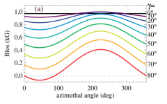
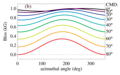
Figure 12.: Variations in expected $B_{\rm los}$ signal from a magnetic vector with $|\mbox{\boldmath$B$}|=1000$G, located at N10, as a function of inherent azimuthal angle $\phi$, while varying (a) the inclination angle $\gamma$ (keeping the heliographic longitude at W10), and (b) varying the heliographic longitude and thus the observing angle (keeping the inherent inclination angle at $10^{\circ}$. fig:bl˙demo

To explore more where the different approaches fail, and how, an analysis of the difference between the $B_{\rm r}$ approximations and the $B_{\rm z}$ component from the vector field observations is performed in detail for one HMI Active Region Patch. HARP 3848, observed by HMI on 2014.03.15 at 15:48:00 TAI includes NOAA AR 12005 and AR 12007 (Figure fig:H3848context), and was centered north-east of disk center; it is one of the regions/days included in the larger HARP dataset, and chosen because of its location, its relatively simple main sunspot plus a second sunspot at a different $\mu$ value, and that it includes a spread of plage over a fair range of $\mu$ as well. The differences between the observed radial component (in this case all using planar approximations) $B_{\rm z}$ and two different $B_{\rm r}$ approximations, from $B_{\rm r}^{\mu(s)}$ and $B_{\rm z}^{\rm pot,center}$ are examined for points in very restrictive local inclination ranges, as a function of structure and observing angle. Two representations are shown: the absolute magnitude (Figure fig:H3848diffs) and the fractional difference (Figure fig:H3848diffs_norm); those points which resulted in an erroneous sign change (relative to the $B_{\rm z}$ boundary) are also indicated. Only points which have a “good” disambiguation and have a signal/noise ratio greater than 5.0 are included.

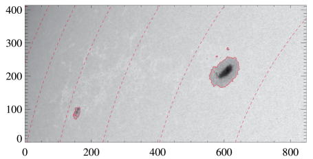
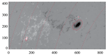
Figure 13.: HARP 3848 (NOAA AR 12005, 12007), obtained at 2014.03.15 at 15:48:00 TAI. Top: continuum intensity, Bottom: radial field $B_{\rm z}$, positive/negative polarity as white/black and scaled to $\pm 2$kG; red contours indicate 0.9 times the median of the continuum intensity and indicate the sunspots, red dashed contours delineate $\mu=0.3,0.4,0.5,0.6,0.7,0.8]$; for reference to Figure fig:H3848diffs.fig:H3848context

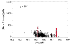
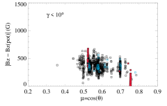
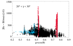
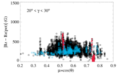
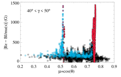
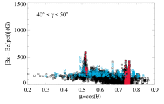
Figure 14.: Top: absolute difference between $B_{\rm z}$ and $B_{\rm r}^{\mu(s)}$(left), and $B_{\rm z}^{\rm pot,center}$ (right), as a function of $\mu=\cos(\theta)$, only for points with local inclination angle $\gamma$ less than $10^{\circ}$ from radial. Points that lie within the spots are indicated by $\ast$ (red). Pixels for which the model resulted in a different sign of the field are further highlighted by over-drawing the squares in blue. Middle, same but for points $20^{\circ}<\gamma<30^{\circ}$; Bottom: same, but for points with $40^{\circ}<\gamma<50^{\circ}$.fig:H3848diffs

Summarizing both plots, for $\gamma<10^{\circ}$, the $B_{\rm r}^{\mu(s)}$ approximation is systematically closer to $B_{\rm z}$ than the $B_{\rm z}^{\rm pot,center}$ results; this is especially true in plage for the $B_{\rm r}^{\mu(s)}$ model, which also shows no sign-error points whereas there are a few sign-error points in the $B_{\rm z}^{\rm pot,center}$ model. For $20^{\circ}<\gamma<30^{\circ}$, slightly inclined fields, the bulk of the points are less different between the two boundaries, however most striking is that the $B_{\rm r}^{\mu(s)}$ approximation is beginning to show significant differences in the sunspots, whereas the $B_{\rm z}^{\rm pot,center}$ sunspot areas continue to display fairly small errors. The latter do, however, show a greater number of plage points which have introduced an erroneous polarity difference whereas the $B_{\rm r}^{\mu(s)}$ shows these errors only at the more extreme $\mu$ values. Examining only points within $40^{\circ}<\gamma<50^{\circ}$ range – significantly inclined but not horizontal – the errors in the spot become very large in $B_{\rm r}^{\mu(s)}$, but stay consistent and small in the $B_{\rm z}^{\rm pot,center}$ boundary. More points in the former are also of the incorrect sign, including many with quite large field-strength differences. The $B_{\rm z}^{\rm pot,center}$ boundary in fact performs better for both plage and spots at these larger inclination angles than $B_{\rm r}^{\mu(s)}$.

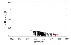
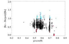
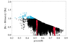
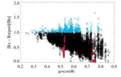
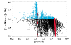
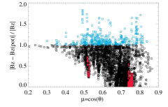
Figure 15.: Same as Figure fig:H3848diffs_norm but each difference is normalized by $|B_{\rm z}|$, to show the fractional change. As such, those points with a sign error (blue-square overplot) will all show a change of at least 100%.fig:H3848diffs˙norm

The appropriateness of a $\mu$-correction in the context of vertical fields is shown thus to be true, but surprisingly limited to a very small degree of deviation away from truly vertical. By 20^∘ from vertical, the results are mixed. For more inclined fields, the $B_{\rm r}^{\mu(s)}$ is clearly problematic, particularly in sunspots (in part due to the (unknown) inherent azimuthal angle), but also in inclined weak-field areas. One must note, however, that what are inferred to be weak-field inclined points may be predominantly a product of noise in the vector field data at these larger observing angles. The $B_{\rm z}^{\rm pot,center}$ boundary is demonstrably better for all inclinations within sunspots, and is susceptible to polarity errors in weak-field areas at all inclinations but at a somewhat more consistent, lower level. In this particular case, the percentage of plage-area pixels with incorrect sign (over all inherent inclination angles) is lower for the $B_{\rm z}^{\rm pot,center}$ boundary than the $B_{\rm r}^{\mu(s)}$ (6.1% vs. 11%, respectively), and the former appears to perform quantitatively better for both plage and spot areas in this example.

5 Conclusions

A method is developed, based on earlier publications [Sakurai (1982), Alissandrakis (1981)], and tested here for its ability to produce an estimate of the radial field distribution from line-of-sight magnetic field observations of the solar photosphere. Comparisons were made between the line-of-sight component calculated from the vector-field observations, the inferred radial-directed component from the same, and different implementations of two approaches for estimating the radial component from line-of-sight observations: one approach based on the common “$\mu$-correction” and one based on using the radial field component from a potential field constructed so as to match the line-of-sight input. The potential-field constructs impose, of course, significant assumptions regarding the underlying structure. The “$\mu$-correction” approach imposes a single much stronger assumption: that the underlying field is always directed normal to the local surface.

We find that answering the question of which approach better recovers a target quantity differs according to said target’s underlying magnetic field structure as would be inferred by the instrument at hand. Structures which abide by the radial-field assumption are well recovered by “$\mu$-correction” approaches. This may, with caution, be extended to structures whose inherent inclination is up to a few tens of degrees, but with an uncertain worsening error as a function of increasing observing angle. Magnetic structures which would be observed to be inherently more inclined by that instrument are generally poorly served by “$\mu$-correction” approaches.

Most active regions comprise a mix of structures, and as such making general performance statements is dangerous. While sunspot field strengths are far better recovered using the potential-field constructs, tests on polar or high-latitude areas that should be primarily plage tell a mixed story: higher field strengths are recovered more reliably using some form of $\mu$-correction, yet results also indicate that a significant subset of the measurements are returned with the incorrect magnetic polarity. That being said, the total magnetic flux, an extensive quantity that often encompasses all structures within an active region, can be better recovered by $\mu$-correction approaches if the target is dominated by field which would expected to be inferred as radial by the instrument involved.

$B_{\rm los}$ images of sunspots often have pronounced “false” magnetic polarity inversion lines; because the $\mu$-correction approaches involve multiplying by a simple scaling factor, they cannot relocate incorrect PILs and instead enhance incorrect-polarity field strengths. This is a particular problem when strong-gradient PILS need to be identified. The potential-field approaches can mitigate the false-PIL problem; the impact was demonstrated on a near-limb active region, but PIL displacement can occur at any location where $\mu\neq 1.0$.

Of course it can be argued that the potential field is not appropriate for magnetically complex active regions, and that linear or non-linear extrapolations would perform even better. Unfortunately, without crucial additional constraints, there is no unique linear or nonlinear force-free field solution to the $B_{\rm los}$ boundary, whereas the potential field provides a unique solution.

The most general conclusions are first, that any correction improves upon the naive $B_{\rm los}=B_{\rm r}$ approach. Second, the $\mu$-corrections recover field strengths in areas inherently comprised of vertical structures (as would be inferred by the instrument), but introduce random errors whose magnitude can be surprisingly large given a sunspot’s proximity to disk center, and these corrections exacerbate the influence of projection-induced sign errors. Lastly, while the potential-field reconstructions will introduce systematic errors, generally underestimating field strengths and introducing new polarity-sign errors in weaker and more radially-directed fields, it recovers well both the radial-component field strengths in sunspots and the locations of the magnetic polarity inversion lines.

Acknowledgements

The authors would like to acknowledge the helpful comments by the referee for this manuscript. The development of the potential-field reconstruction codes and the preparation of this manuscript was supported by NASA through contracts NNH12CH10C, NNH12CC03C, and grant NNX14AD45G. This material is based upon work supported by the National Science Foundation under Grant No. 0454610. Any opinions, findings, and conclusions or recommendations expressed in this material are those of the author(s) and do not necessarily reflect the views of the National Science Foundation.

Appendix A Method: Planar Approximation

app:method_planar

The line-of-sight component is observed on an image-coordinate planar grid. To avoid having to interpolate to a regular heliographic grid, consider a hybrid (non-orthogonal) coordinate system, $(\xi,\eta,z^{h})$, consisting of the transverse image components, $(\xi,\eta)$ and the heliographic normal component, $z^{h}$.

Following the convention of garyhagyard90, the coordinates $\xi$, $\eta$ are defined in the $z^{h}=0$ plane in terms of heliographic coordinates by

$$\left(\begin{array}[]{c}\xi\\ \eta\end{array}\right) = \left(\begin{array}[]{cc}c_{11}&c_{12}\\ c_{21}&c_{22}\end{array}\right)\left(\begin{array}[]{c}x^{h}\\ y^{h}\end{array}\right).$$ (14)

thus the new coordinate system is related to helioplanar coordinates by

$$\left(\begin{array}[]{c}\xi\\ \eta\\ z^{h}\end{array}\right) = \left(\begin{array}[]{ccc}c_{11}&c_{12}&0\\ c_{21}&c_{22}&0\\ 0&0&1\end{array}\right)\left(\begin{array}[]{c}x^{h}\\ y^{h}\\ z^{h}\end{array}\right).$$ (24)

Hence, the calculations are performed in the coordinate system $(\xi,\eta,z)$, which is not the same as the image coordinates, except at $z=0$. As such, there will be three coordinate systems under consideration, related as follows. The heliographic and image coordinates are related by the standard transform given in garyhagyard90:

$$\left(\begin{array}[]{c}x^{h}\\ y^{h}\\ z^{h}\end{array}\right) = \left(\begin{array}[]{ccc}a_{11}&a_{12}&a_{13}\\ a_{21}&a_{22}&a_{23}\\ a_{31}&a_{32}&a_{33}\end{array}\right)\left(\begin{array}[]{c}x^{i}\\ y^{i}\\ z^{i}\end{array}\right),$$ (34)

while the new coordinate system is related to the originals by

$$\left(\begin{array}[]{c}\xi\\ \eta\\ z\end{array}\right) = \left(\begin{array}[]{ccc}c_{11}&c_{12}&0\\ c_{21}&c_{22}&0\\ 0&0&1\end{array}\right)\left(\begin{array}[]{c}x^{h}\\ y^{h}\\ z^{h}\end{array}\right),$$ (44)

$$= \left(\begin{array}[]{ccc}c_{11}a_{11}+c_{12}a_{21}&c_{11}a_{12}+c_{12}a_{22}&c_{11}a_{13}+c_{12}a_{23}\\ c_{21}a_{11}+c_{22}a_{21}&c_{21}a_{12}+c_{22}a_{22}&c_{21}a_{13}+c_{22}a_{23}\\ a_{31}&a_{32}&a_{33}\end{array}\right)\left(\begin{array}[]{c}x^{i}\\ y^{i}\\ z^{i}\end{array}\right).$$ (51)

Henceforth, the superscript on the heliographic components is dropped, but retained on the image components.

The volume of interest is restricted to $0<\xi<L_{x}$, $0<\eta<L_{y}$ and $z\geq 0$. Assuming that $c_{ij}$ is constant (that is, neglecting curvature across the field of view), this transformation is linear and the solution to Laplace’s equation should still be of the form

$$\Phi(\xi,\eta,z) = \sum_{m,n}A_{mn}e^{[2\pi im\xi/L_{x}+2\pi in\eta/L_{y}-\kappa_{mn}z]}+A_{\xi}\xi+A_{\eta}\eta+A_{0}z,$$ (52)

with the value of $\kappa_{mn}$ determined by $\mbox{\boldmath$\nabla$}^{2}\Phi=0$, namely

$$\mbox{\boldmath$\nabla$}^{2}\Phi(\xi,\eta,z) = {\partial^{2}\Phi\over\partial\xi^{2}}\bigg{[}\bigg{(}{d\xi\over dx}\bigg{)}^{2}+\bigg{(}{d\xi\over dy}\bigg{)}^{2}\bigg{]}+2{\partial^{2}\Phi\over\partial\xi\partial\eta}\bigg{[}{d\xi\over dx}{d\eta\over dx}+{d\xi\over dy}{d\eta\over dy}\bigg{]}$$

$$+{\partial^{2}\Phi\over\partial\eta^{2}}\bigg{[}\bigg{(}{d\eta\over dx}\bigg{)}^{2}+\bigg{(}{d\eta\over dy}\bigg{)}^{2}\bigg{]}+{\partial^{2}\Phi\over\partial z^{2}}$$

$$= \sum_{m,n}A_{mn}e^{[2\pi im\xi/L_{x}+2\pi in\eta/L_{y}-\kappa_{mn}z]}\bigg{\{}(c_{11}^{2}+c_{12}^{2})\bigg{(}{2\pi im\over L_{x}}\bigg{)}^{2}$$

$$\qquad+2(c_{11}c_{21}+c_{12}c_{22})\bigg{(}{2\pi im\over L_{x}}\bigg{)}\bigg{(}{2\pi in\over L_{y}}\bigg{)}$$

$$\qquad+(c_{21}^{2}+c_{22}^{2})\bigg{(}{2\pi in\over L_{y}}\bigg{)}^{2}+\kappa_{mn}^{2}\bigg{\}}$$

$$\Rightarrow\ \kappa_{mn}^{2} = (2\pi)^{2}\bigg{[}(c_{11}^{2}+c_{12}^{2})\bigg{(}{m\over L_{x}}\bigg{)}^{2}+2(c_{11}c_{21}+c_{12}c_{22})\bigg{(}{m\over L_{x}}\bigg{)}\bigg{(}{n\over L_{y}}\bigg{)}$$ (53)

$$\qquad+(c_{21}^{2}+c_{22}^{2})\bigg{(}{n\over L_{y}}\bigg{)}^{2}\bigg{]}$$

and choose $\kappa_{mn}>0$ so the field decreases with height. Also choose $A_{\xi}=A_{\eta}=0$, so the constant field is purely vertical. This is equivalent to specifying the boundary condition at large heights.

The line of sight component of the field is thus given by

$$B_{l} = {\partial\over\partial x_{l}}\bigg{\{}\sum_{m,n}A_{mn}e^{2\pi im\xi/L_{x}+2\pi in\eta/L_{y}-\kappa_{mn}z}+A_{0}z\bigg{\}}$$ (54)

$$= a_{33}A_{0}+\sum_{m,n}A_{mn}e^{2\pi im\xi/L_{x}+2\pi in\eta/L_{y}-\kappa_{mn}z}$$

$$\qquad\times\bigg{[}{2\pi im\over L_{x}}(c_{11}a_{13}+c_{12}a_{23})+{2\pi in\over L_{y}}(c_{21}a_{13}+c_{22}a_{23})-\kappa_{mn}a_{33}\bigg{]}.$$

Solve for the coefficients $A_{mn}$ by taking the Fourier transform of the line of sight component of the field at the surface

$${\tt FFT}(B^{l}) = \int_{0}^{L_{x}}d\xi\,\int_{0}^{L_{y}}d\eta\,B_{l}(\xi,\eta,0)e^{-2\pi ij\xi/L_{x}-2\pi ik\eta/L_{y}}$$ (55)

$$= \sum_{m,n}A_{mn}\bigg{[}{2\pi im\over L_{x}}(c_{11}a_{13}+c_{12}a_{23})+{2\pi in\over L_{y}}(c_{21}a_{13}+c_{22}a_{23})-\kappa_{mn}a_{33}\bigg{]}$$

$$\qquad\times\int_{0}^{L_{x}}d\xi\int_{0}^{L_{y}}d\eta e^{2\pi i(m-j)\xi/L_{x}+2\pi i(n-k)\eta/L_{y}}$$

$$\quad+A_{0}{\partial z\over\partial x_{l}}\int_{0}^{L_{x}}d\xi\,\int_{0}^{L_{y}}d\eta\,e^{-2\pi ij\xi/L_{x}-2\pi ik\eta/L_{y}}$$

$$= {L_{x}}{L_{y}}A_{jk}\bigg{[}{2\pi ij\over L_{x}}(c_{11}a_{13}+c_{12}a_{23})+{2\pi ik\over L_{y}}(c_{21}a_{13}+c_{22}a_{23})-\kappa_{jk}a_{33}\bigg{]}$$

$$\quad+L_{x}L_{y}a_{33}A_{0}\delta_{0j}\delta_{0k}.$$

Knowing the coefficients, the vertical component of the field is given by

$$B_{z}(\xi,\eta,0) = {\partial\over\partial z}\bigg{\{}\sum_{m,n}A_{mn}e^{2\pi im\xi/L_{x}+2\pi in\eta/L_{y}-\kappa_{mn}z}+A_{0}z\bigg{\}}\bigg{|}_{z=0}$$ (56)

$$= A_{0}-\sum_{m,n}\kappa_{mn}A_{mn}e^{2\pi im\xi/L_{x}+2\pi in\eta/L_{y}}.$$

Appendix B Method: Spherical Case

app:method_spherical

Following the derivation given in altschulernewkirk69, but also see Bogdan86, the potential field in a semi-infinite volume $r\geq R$ can be written in terms of a scalar potential given by

$$\Psi = R\sum_{n=1}^{\infty}\sum_{m=0}^{n}\bigg{(}{R\over r}\bigg{)}^{n+1}(g_{n}^{m}\cos m\phi+h_{n}^{m}\sin m\phi)P_{n}^{m}(\mu),$$ (57)

where $\mu=\cos\theta$, in terms of which the heliographic components of the field are given by

$$B_{r} = -{\partial\Psi\over\partial r}$$ (58)

$$= \sum_{n=1}^{\infty}\sum_{m=0}^{n}(n+1)\bigg{(}{R\over r}\bigg{)}^{n+2}(g_{n}^{m}\cos m\phi+h_{n}^{m}\sin m\phi)P_{n}^{m}(\mu),$$

$$B_{\theta} = -{1\over r}{\partial\Psi\over\partial\theta}$$ (59)

$$= {1\over\sin\theta}\sum_{n=1}^{\infty}\sum_{m=0}^{n}\bigg{(}{R\over r}\bigg{)}^{n+2}(g_{n}^{m}\cos m\phi+h_{n}^{m}\sin m\phi)$$

$$\qquad\times\bigg{[}(n+1)\mu P_{n}^{m}(\mu)-(n-m+1)P_{n+1}^{m}(\mu)\bigg{]}$$

$$B_{\phi} = -{1\over r\sin\theta}{\partial\Psi\over\partial\phi}$$ (60)

$$= {1\over\sin\theta}\sum_{n=1}^{\infty}\sum_{m=0}^{n}m\bigg{(}{R\over r}\bigg{)}^{n+2}(g_{n}^{m}\sin m\phi-h_{n}^{m}\cos m\phi)P_{n}^{m}(\mu).$$

Following Rudenko2001a, define the coordinate system such that the line of sight direction corresponds to the polar axis of the expansion. With this choice, the line of sight component of the field is given by

eqn:Blos$$B_{l} = B_{r}\cos\theta-B_{\theta}\sin\theta.$$ (61)

$$= \sum_{n=1}^{\infty}\sum_{m=0}^{n}(n-m+1)\bigg{(}{R\over r}\bigg{)}^{n+2}P_{n+1}^{m}(\mu)\bigg{[}g_{n}^{m}\cos m\phi+h_{n}^{m}\sin m\phi\bigg{]}.$$

To determine the coefficients in the expansion, first multiple both sides of equation eqn:Blos by $\cos m\theta$, and integrate over the surface of the sphere of radius $R$:

$$\int_{0}^{\pi}\sin\theta d\theta\int_{0}^{2\pi}d\phi\,\cos m\phi P_{n+1}^{m}(\mu)B_{l}(R,\theta,\phi)$$ (62)

$$= \sum_{n^{\prime}=1}^{\infty}\sum_{m^{\prime}=0}^{n^{\prime}}\int_{0}^{\pi}\sin\theta d\theta\int_{0}^{2\pi}d\phi\,\cos m\phi(n^{\prime}-m^{\prime}+1)P_{n+1}^{m}(\mu)P_{n^{\prime}+1}^{m^{\prime}}(\mu)$$

$$\quad\times\bigg{[}g_{n^{\prime}}^{m^{\prime}}\cos m^{\prime}\phi+h_{n^{\prime}}^{m^{\prime}}\sin m^{\prime}\phi\bigg{]}$$

$$= {4\pi g_{n}^{m}\over 2n+3}{(n+m+1)!\over(n-m)!},$$

which determines $g_{n}^{m}$. Next, multiply both sides of equation eqn:Blos by $\sin m\theta$, and again integrate over the surface of the sphere of radius $R$:

$$\int_{0}^{\pi}\sin\theta d\theta\int_{0}^{2\pi}d\phi\,\sin m\phi P_{n+1}^{m}(\mu)B_{l}(R,\theta,\phi)$$ (63)

$$= \sum_{n^{\prime}=1}^{\infty}\sum_{m^{\prime}=0}^{n^{\prime}}\int_{0}^{\pi}\sin\theta d\theta\int_{0}^{2\pi}d\phi\,\sin m\phi(n^{\prime}-m^{\prime}+1)P_{n+1}^{m}(\mu)P_{n^{\prime}+1}^{m^{\prime}}(\mu)$$

$$\quad\times\bigg{[}g_{n^{\prime}}^{m^{\prime}}\cos m^{\prime}\phi+h_{n^{\prime}}^{m^{\prime}}\sin m^{\prime}\phi\bigg{]}$$

$$= {4\pi h_{n}^{m}\over 2n+3}{(n+m+1)!\over(n-m)!}$$

to determine $h_{n}^{m}$.

Because observations are only available for the near side of the Sun, to actually implement this, it is necessary to make an assumption about the far side of the Sun. In order to ensure a zero monopole moment, it is convenient to make the field anti-symmetric in some form. One convenient way to do this is to let $B_{l}(R,\pi-\theta,\phi)=B_{l}(R,\theta,\phi)$, where the front side of the Sun is assumed to lie in the range $0<\theta<\pi/2$. Using the fact that the associated Legendre functions have the property

$$P_{n}^{m}(-x) = (-1)^{(n+m)}P_{n}^{m}(x),$$ (64)

the expressions for the coefficients become

$$g_{n}^{m} = {(2n+3)(n-m)!\over 4\pi(n+m+1)!}\int_{0}^{2\pi}d\phi\,\cos m\phi$$ (65)

$$\qquad\times\bigg{\{}\int_{-1}^{0}d\mu\,P_{n+1}^{m}(\mu)+\int_{0}^{1}d\mu\,P_{n+1}^{m}(\mu)\bigg{\}}B_{l}(R,\mu,\phi)$$

$$= {(2n+3)(n-m)![1+(-1)^{n+m+1}]\over 4\pi(n+m+1)!}$$

$$\qquad\times\int_{0}^{2\pi}d\phi\,\cos m\phi\int_{0}^{1}d\mu\,P_{n+1}^{m}(\mu)B_{l}(R,\mu,\phi)$$

and similarly

$$h_{n}^{m} = {(2n+3)(n-m)![1+(-1)^{n+m+1}]\over 4\pi(n+m+1)!}$$ (66)

$$\qquad\times\int_{0}^{2\pi}d\phi\,\sin m\phi\int_{0}^{1}d\mu\,P_{n+1}^{m}(\mu)B_{l}(R,\mu,\phi).$$

Note that the terms with $n+m$ even have $g_{n}^{m}=h_{n}^{m}=0$. This is a consequence of the boundary condition imposed for the far side of the Sun, which effectively reduces the number of independent terms by a factor of two.

References

- Alissandrakis (1981) Alissandrakis, C.E.: 1981, A&A 100, 197.
- Altschuler and Newkirk (1969) Altschuler, M.D., Newkirk, G.: 1969, Sol. Phys. 9, 131. doi:10.1007/BF00145734.
- Barnes et al. (2017) Barnes, G., Leka, K.D., Crouch, A.D., Sun, X., Wagner, E.L., Schou, J.: 2017, Sol. Phys. in preparation.
- Bobra et al. (2014) Bobra, M.G., Sun, X., Hoeksema, J.T., Turmon, M., Liu, Y., Hayashi, K., Barnes, G., Leka, K.D.: 2014, Sol. Phys. 289, 3549. doi:10.1007/s11207-014-0529-3.
- Bogdan (1986) Bogdan, T.J.: 1986, Sol. Phys. 103, 311. doi:10.1007/BF00147832.
- Centeno et al. (2014) Centeno, R., Schou, J., Hayashi, K., Norton, A., Hoeksema, J.T., Liu, Y., Leka, K.D., Barnes, G.: 2014, Sol. Phys. 289, 3531. doi:10.1007/s11207-014-0497-7.
- Chapman and Sheeley (1968) Chapman, G.A., Sheeley, N.R. Jr.: 1968, In: Kiepenheuer, K.O. (ed.) Structure and Development of Solar Active Regions, IAU Symposium 35, 161.
- Gary and Hagyard (1990) Gary, G.A., Hagyard, M.J.: 1990, Sol. Phys. 126, 21.
- Giovanelli (1980) Giovanelli, R.G.: 1980, Sol. Phys. 68, 49. doi:10.1007/BF00153266.
- Hoeksema et al. (2014) Hoeksema, J.T., Liu, Y., Hayashi, K., Sun, X., Schou, J., Couvidat, S., Norton, A., Bobra, M., Centeno, R., Leka, K.D., Barnes, G., Turmon, M.: 2014, Sol. Phys. 289, 3483. doi:10.1007/s11207-014-0516-8.
- Ito et al. (2010) Ito, H., Tsuneta, S., Shiota, D., Tokumaru, M., Fujiki, K.: 2010, ApJ 719, 131. doi:10.1088/0004-637X.
- Jones (1985) Jones, H.P.: 1985, Australian Journal of Physics 38, 919.
- Keller and The Solis Team (2001) Keller, C.U., The Solis Team: 2001, In: Sigwarth, M. (ed.) Advanced Solar Polarimetry – Theory, Observation, and Instrumentation, Astronomical Society of the Pacific Conference Series 236, 16.
- Leka et al. (2009) Leka, K.D., Barnes, G., Crouch, A.D., Metcalf, T.R., Gary, G.A., Jing, J., Liu, Y.: 2009, Sol. Phys. 260, 83. doi:10.1007/s11207-009-9440-8.
- Livshits et al. (2015) Livshits, M.A., Rudenko, G.V., Katsova, M.M., Myshyakov, I.I.: 2015, Advances in Space Research 55, 920. doi:10.1016/j.asr.2014.08.026.
- Pesnell (2008) Pesnell, W.: 2008, In: 37th COSPAR Scientific Assembly, COSPAR, Plenary Meeting 37, 2412.
- Petrie (2015) Petrie, G.J.D.: 2015, Living Reviews in Solar Physics 12. doi:10.1007/lrsp-2015-5.
- Pope and Mosher (1975) Pope, T., Mosher, J.: 1975, Sol. Phys. 44, 3. doi:10.1007/BF00156842.
- Riley et al. (2006) Riley, P., Linker, J.A., Mikić, Z., Lionello, R., Ledvina, S.A., Luhmann, J.G.: 2006, ApJ 653, 1510. doi:10.1086/508565.
- Riley et al. (2014) Riley, P., Ben-Nun, M., Linker, J.A., Mikic, Z., Svalgaard, L., Harvey, J., Bertello, L., Hoeksema, T., Liu, Y., Ulrich, R.: 2014, Sol. Phys. 289, 769. doi:10.1007/s11207-013-0353-1.
- Rudenko (2001) Rudenko, G.V.: 2001, Sol. Phys. 198, 5.
- Sainz Dalda and Martínez Pillet (2005) Sainz Dalda, A., Martínez Pillet, V.: 2005, ApJ 632, 1176. doi:10.1086/433168.
- Sakurai (1982) Sakurai, T.: 1982, Sol. Phys. 76, 301. doi:10.1007/BF00170988.
- Scherrer et al. (2012) Scherrer, P.H., Schou, J., Bush, R.I., Kosovichev, A.G., Bogart, R.S., Hoeksema, J.T., Liu, Y., Duvall, T.L., Zhao, J., Title, A.M., Schrijver, C.J., Tarbell, T.D., Tomczyk, S.: 2012, Sol. Phys. 275, 207. doi:10.1007/s11207-011-9834-2.
- Schrijver (2007) Schrijver, C.J.: 2007, ApJL 655, 117. doi:10.1086/511857.
- Svalgaard, Duvall, and Scherrer (1978) Svalgaard, L., Duvall, T.L. Jr., Scherrer, P.H.: 1978, Sol. Phys. 58, 225. doi:10.1007/BF00157268.
- Tsuneta et al. (2008) Tsuneta, S., Ichimoto, K., Katsukawa, Y., Lites, B.W., Matsuzaki, K., Nagata, S., Orozco Suárez, D., Shimizu, T., Shimojo, M., Shine, R.A., Suematsu, Y., Suzuki, T.K., Tarbell, T.D., Title, A.M.: 2008, ApJ 688, 1374. doi:10.1086/592226.
- Wang and Sheeley (1992) Wang, Y., Sheeley, J.N.R.: 1992, ApJ 392, 310. doi:10.1086/171430.
- Wieczorek et al. (2016) Wieczorek, M.A., Meschede, M., Oshchepkov, I., Sales de Andrade, E.: 2016, Zenodo. doi:10.5281/zenodo.61180.