Abstract

We consider implementations of high-order finite difference Weighted Essentially Non-Oscillatory (WENO) schemes for the Euler equations in cylindrical and spherical coordinate systems with radial dependence only. The main concern of this work lies in ensuring both high-order accuracy and conservation. Three different spatial discretizations are assessed: one that is shown to be high-order accurate but not conservative, one conservative but not high-order accurate, and a new approach that is both high-order accurate and conservative. For cylindrical and spherical coordinates, we present convergence results for the advection equation and the Euler equations with an acoustics problem; we then use the Sod shock tube and the Sedov point-blast problems in cylindrical coordinates to verify our analysis and implementations.

1 Introduction

In a variety of physical phenomena, the dominant dynamics occur in spherical and cylindrical geometries. Examples include astrophysics (e.g., supernova collapse), nuclear explosions, inertial confinement fusion (ICF) and cavitation-bubble dynamics. A natural approach to solving these problems is to write the governing equations in cylindrical/spherical coordinates, which can then be solved numerically using an appropriate discretization. Historically, the first such numerical studies were conducted by Von Neumann and Richtmyer [22] in the 1940s for nuclear explosions. To treat the discontinuities in a stable fashion, they explicitly introduced artificial dissipation to the Euler equations. While this method correctly captures the position of shocks and satisfies the Rankine-Hugoniot equations, flow features in the numerical solution, in particular discontinuities, are smeared due to excessive dissipation.

The collapse and explosion of cavitation bubbles, supernovae and ICF capsules share similarities in that they are all, under ideal circumstances, spherically symmetric flows that involve material interfaces and shock waves. Such flows are rarely ideal, insofar as they are prone to interfacial instabilities due to accelerations (Rayleigh-Taylor [18]), shocks (Richtmyer-Meshkov [4]), or geometry (Bell-Plesset [3, 17]). When solving problems with large three-dimensional perturbations, cylindrical/spherical coordinates may not be advantageous. However, in certain problems such as sonoluminescence [2], the spherical symmetry assumption is remarkably valid. Modeling the bubble motion with spherical symmetry can greatly reduce the computational cost. As an example, Akhatov, et al. [1] used a first-order Godunov scheme to simulate liquid flow outside of a single bubble whose radius was given by the Rayleigh-Plesset equation. This approach assumes spherical symmetry but does not solve the equations of motion inside the bubble.

High-order accurate methods are becoming mainstream in computational fluid dynamics [23]. However, implementation of such methods in cylindrical/spherical geometries is not trivial. Several recent studies in cylindrical and spherical coordinates have focused on the Lagrangian form of the equations [14, 21]. The Euler equations in cylindrical or spherical geometry were studied by Maire [14] using a cell-centered Lagrangian scheme, which ensures conservation of momentum and energy. These equations were also considered by Omang et al. [16] using Smoothed Particle Hydrodynamics (SPH), though SPH methods are generally not high-order accurate. On the other hand, solving the equations in Eulerian form is not trivial, especially when trying to ensure conservation and high-order accuracy. Li [12] attempted to implement Eulerian finite difference and finite volume weighted essentially non-oscillatory (WENO) schemes [8] on cylindrical and spherical grids, but did not achieve satisfactory results in terms of accuracy and conservation. Liu et al. [7] considered flux difference-splitting methods for ducts with area variation. [13] followed a similar formulation of the equations employing a total variation diminishing method to simulate explosions in air. Johnsen & Colonius [10, 11] used cylindrical coordinates with azimuthal symmetry to simulate the collapse of an initially spherical gas bubble in shock-wave lithotripsy by solving the Euler equations inside and outside the bubble using WENO. De Santis [5] showed equivalence between their Lagrangian finite element and finite volume schemes in cylindrical coordinates. Xing and Shu [24, 25, 26] performed extensive studies of hyperbolic systems with source terms, which are relevant as the equations in cylindrical/spherical coordinates can be written with geometrical source terms. Although one of their test cases involved radial flow in a nozzle using the quasi one-dimensional nozzle flow equations, they did not consider the general gas dynamics equations. Thus, at this time, a systematic study of the Euler equations in cylindrical and spherical coordinates, with respect to order of accuracy and conservation, has yet to be conducted.

In this paper, we investigate three different spatial discretizations in cylindrical/spherical coordinates with radial dependence only using finite difference WENO schemes for the Euler equations. In particular, we propose a new approach that is both high-order accurate and conservative. Here, we are concerned with the interior scheme; appropriate boundary approaches will be investigated in a later study. The governing equations are stated in Section 2 and the spatial discretizations are presented in Section 3. In Section 4, we test the different discretizations on smooth problems (scalar advection equation, acoustics problem for the Euler equations) for convergence, and with shock-dominated problems (Sod shock tube and Sedov point blast problems) for conservation. The last section summarizes the present work and provides a future outlook.

2 Governing equations

The differential for the Euler equations in cylindrical/spherical coordinates with radial dependence only:

$$\frac{\partial\mathbf{U}}{\partial t}+\frac{1}{r^{\alpha}}\frac{\partial\left(r^{\alpha}\mathbf{F}(\mathbf{U})\right)}{\partial r}=\mathbf{S}(\mathbf{U})$$ (1)

where $\mathbf{U}=(\rho,m=\rho u,E)^{T}$, $\mathbf{F}(\mathbf{U})=\left(m,\frac{m^{2}}{\rho}+p,\frac{m}{\rho}(E+p)\right)^{T}$, and $\mathbf{S}(\mathbf{U})=(0,p,0)^{T}$. $\rho$ is the density, u is velocity in radial direction, $t$ is time, $r$ is the radial coordinate, $p$ is the pressure, $E$ is the total energy per unit volume, and $\alpha$ is a geometrical parameter, which is 0, 1, or 2 for Cartesian, cylindrical, or spherical coordinates, respectively. Subscripts denote derivatives. Diffusion effects are neglected. For an ideal gas, the equation of state to close this system can be written:

$$p=\left(\gamma-1\right)\varepsilon,$$ (2)

where $\varepsilon=E-\rho u^{2}/2$ is the internal energy per unit volume, and $\gamma$ is the specific heats ratio. Other equations of state can be used, e.g., a stiffened equation for liquids and solids.

3 Numerical method

We describe three discretizations of the Euler Eqs.(1) in cylindrical/spherical coordinates that differ based on the treatment of the convective terms. While the discretized form of the Euler equations in Cartesian coordinates is generally designed to conserve mass, momentum and energy, the conservation condition does not necessarily hold in cylindrical or spherical coordinates, depending on the numerical treatment of the equations. The criterion we use to determine discrete conservation is as follows:

$$\int_{\Omega}\phi(t,r)dv=\int_{\Omega}\phi(0,r)dv,$$ (3)

where $\Omega$ is a domain (possibly a computational cell). Here, $\phi$ represents a conserved variable, e.g., density, momentum per unit volume or energy per unit volume. This equation means that the total mass, momentum, and energy are constant in time provided there is no flux of these quantities through the boundaries of the domain, which is the case for the problems of interest here. A different approach to defining conservation for hyperbolic laws is the exact C-type property [24], which implies that the system admits a stationary solution in which nonzero flux gradients are exactly balanced by the source terms in the steady-state case. Xing and Shu [25, 26] applied WENO in systems of conservation laws with source terms and considered radial flow in a nozzle using the quasi one-dimensional nozzle flow equations. In our work, we focus on the Euler equations.

We consider finite difference(FD) WENO schemes. we give brief description of a fifth-order finite difference WENO scheme is given in Appendix. For finite difference WENO, given the cell-centered values, the fluxes are first split and then interpolated to compute the numerical flux. In order to give a clear image of implementation, we write the solution procedure right after describing the spatial discretization for each method.

Method One

The first spatial discretization, labelled Method One here, can be found in Chapter 1.6 of Toro [20]. Expand the convective term and move the part without spatial derivative to right hand of Eq. 1 to obtain the differential equations

$$\frac{\partial\mathbf{U}}{\partial t}+\frac{\partial\mathbf{F}(\mathbf{U})}{\partial r}=\mathbf{S}(\mathbf{U})-\frac{\alpha}{r}\mathbf{F}(\mathbf{U})$$ (4)

The notation is consistent with the notation in Eq. 1.

For the convenience of programming, we also write the mass, momentum and energy in semi-discrete form:

$$\frac{\mathrm{d}\rho_{i}}{\mathrm{d}t}= -\frac{(\rho u)_{i+1/2}-(\rho u)_{i-1/2}}{\Delta r_{i}}-\frac{\alpha}{r_{i}}\left(\rho u\right)_{i},$$ (5a)

$$\frac{\mathrm{d}(\rho u)_{i}}{\mathrm{d}t}= -\frac{(\rho u+p)_{i+1/2}-(\rho u+p)_{i-1/2}}{\Delta r_{i}}-\frac{\alpha}{r_{i}}\left(\rho u^{2}\right)_{i},$$ (5b)

$$\frac{\mathrm{d}E_{i}}{\mathrm{d}t}= -\frac{[(E+p)u]_{i+1/2}-[(E+p)u]_{i-1/2}}{\Delta r_{i}}-\frac{\alpha}{r_{i}}\left[u(E+p)\right]_{i},$$ (5c)

where $\Delta r_{i}$ is the linear radial cell width. For FD WENO, the variables to be evolved in time are the cell-centered values, i.e., the values at $r_{i}$ in cell $[r_{i-1/2},r_{i+1/2}]$.

With this approach derived from the differential form of the equations rather than the integral, physical variables expected to be conserved are not necessarily conserved numerically because there is no strict constraint between the conservative fluxes and the geometrical source terms. However, high-order accuracy may be achieved with this method.

This part summarizes the solution procedure for Method One used in our code:
1. Initialize the primitive variables, $\rho$, $u$, $p$, and $E$
2. Using local Lax-Fredrich to split the flux, obtain $\rho u_{i}^{\pm}$, $(\rho u+p)_{i}^{\pm}$ , $[(E+p)u]_{i}^{\pm}$, and local speed of wind, $\lambda_{i}$. The plus sign means the flux moves toward right, the minus sign means the flux moves toward left. The convention is used in all the flux calculation part in this paper.
3. Using the local characteristic decomposition and finite difference WENO to approximate the flux, obtain $\rho u_{i+1/2}^{\pm}$ , $(\rho u+p)_{i+1/2}^{\pm}$ , and $[(E+p)u]_{i+1/2}^{\pm}$.
4. Calculate the residual. The source terms in Method one are collocated with primitive variable, can be directly added to the residual. Note that the source terms are updated in each sub-step.
5. March in time.

Method Two

The second discretization, Method Two, is based on the integral form of the equations and was used by several authors [7, 13, 10]. The mass, momentum and energy equations are written in semi-discrete form:

$$\frac{\mathrm{d}\rho_{i}}{\mathrm{d}t}= -\frac{r_{i+1/2}^{\alpha}(\rho u)_{i+1/2}-r_{i-1/2}^{\alpha}(\rho u)_{i-1/2}}{\Delta V_{i}},$$ (6a)

$$\frac{\mathrm{d}(\rho u)_{i}}{\mathrm{d}t}= -\frac{r_{i+1/2}^{\alpha}(\rho u^{2}+p)_{i+1/2}-r_{i-1/2}^{\alpha}(\rho u^{2}+p)_{i-1/2}}{\Delta V_{i}}+S(r_{i}),$$ (6b)

$$\frac{\mathrm{d}E_{i}}{\mathrm{d}t}= -\frac{r_{i+1/2}^{\alpha}[(E+p)u]_{i+1/2}-r_{i-1/2}^{\alpha}[(E+p)u]_{i-1/2}}{\Delta V_{i}},$$ (6c)

where $\Delta V_{i}=\frac{1}{1+\alpha}(r_{i+1/2}^{\alpha+1}-r_{i-1/2}^{\alpha+1})$ and $S(r_{i})$ is the source term in the momentum equation, which can be expressed as:

$$S(r_{i})=\frac{r_{i+1/2}^{\alpha}p_{i+1/2}-r_{i-1/2}^{\alpha}p_{i-1/2}}{\Delta V_{i}}-\frac{p_{i+1/2}-p_{i-1/2}}{\Delta r}.$$ (7)

Depending on the reconstruction procedure, the first term may cancel the corresponding term in the momentum equation. Again, the variables to be evolved in time are the cell-centered values for FD WENO.

With this approach, the relevant physical variables are expected to be conserved. However, the order accuracy is ultimately second order. This latter point can be readily understood by subtracting Method Two from Method One:

$$\frac{f_{j+1/2}r_{j+1/2}^{\alpha}-f_{j-1/2}r_{j-1/2}^{\alpha}}{\frac{1}{\alpha+1}(r_{j+1/2}^{\alpha+1}-r_{j-1/2}^{\alpha+1})}-\left(\frac{f_{j+1/2}-f_{j-1/2}}{\Delta r}+\frac{\alpha f_{j}}{r_{j}}\right)=O(\Delta r^{2}).$$ (8)

This part summarizes the solution procedure for Method Two used in our code:
1. Initialize the primitive variables, $\rho$, $u$, $p$, and $E$
2. Using local Lax-Fredrich to split the flux, obtain $\rho u_{i}^{\pm}$, $(\rho u+p)_{i}^{\pm}$ , $[(E+p)u]_{i}^{\pm}$, and local speed of wind, $\lambda_{i}$.
3. Using the local characteristic decomposition and finite difference WENO to approximate the flux, obtain $\rho u_{i\pm 1/2}^{\pm}$ , $(\rho u+p)_{i\pm 1/2}^{\pm}$ , and $[(E+p)u]_{i\pm 1/2}^{\pm}$.
4. Calculate the residual. The source terms in Method Two are located at the cell surface. It is not straight forward to calculate it form $\rho u_{i\pm 1/2}^{\pm}$ , $(\rho u+p)_{i\pm 1/2}^{\pm}$ , and $[(E+p)u]_{i\pm 1/2}^{\pm}$. Our solution is to approximate $p_{i\pm 1/2}^{\pm}$ using the same nonlinear weights. The source terms are updated in each sub-step.
5. March in time.

Method Three

The third spatial discretization, Method Three, is inspired by the solution to acoustics problems in spherical coordinates. This approach is also used by Toro [20] and Zhang[27]. Multiplying Eqs. (1) by $r^{\alpha}$,

$$\frac{\partial(r^{\alpha}\mathbf{U})}{\partial t}+\frac{\partial\left(r^{\alpha}\mathbf{F}(\mathbf{U})\right)}{\partial r}=r^{\alpha}\mathbf{S}(\mathbf{U})$$ (9)

For the convenience of programming, the mass, momentum, and energy equations are written in semi-discrete form:

$$\frac{\mathrm{d}(r^{\alpha}\rho)_{i}}{\mathrm{d}t}= -\frac{(r^{\alpha}\rho u)_{i+1/2}-(r^{\alpha}\rho u)_{i-1/2}}{\Delta r_{i}},$$ (10a)

$$\frac{\mathrm{d}(r^{\alpha}\rho u)_{i}}{\mathrm{d}t}= -\frac{[r^{\alpha}(\rho u^{2}+p)]_{i+1/2}-[r^{\alpha}(\rho u^{2}+p)]_{i-1/2}}{\Delta r_{i}}+\alpha(pr^{\alpha-1})_{i},$$ (10b)

$$\frac{\mathrm{d}(r^{\alpha}E)_{i}}{\mathrm{d}t}= -\frac{[r^{\alpha}(E+p)u]_{i+1/2}-[r^{\alpha}(E+p)u]_{i-1/2}}{\Delta r_{i}}.$$ (10c)

For FD WENO, the cell-centered values are considered. This approach strictly follows the integral form of the Euler equations in cylindrical or spherical coordinates and satisfies the C-type property for hyperbolic equations with source terms [24]. Thus, it is expected to be both conservative and high-order accurate.

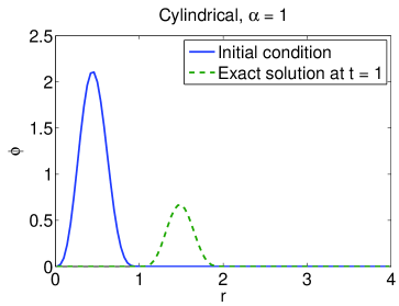
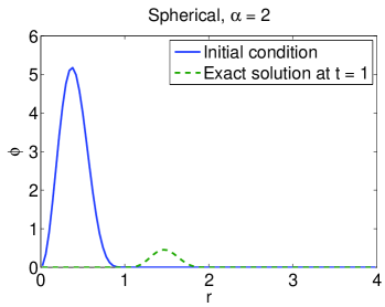
Figure 1: Initial conditions and exact solution after $t=1$ for the advection equation.

This part summarizes the solution procedure for Method Two used in our code:
1. Initialize the primitive variables, $\rho$, $u$, $p$, and $E$, then calculate $r^{\alpha}\rho$, $r^{\alpha}u$, $r^{\alpha}p$, and $r^{\alpha}E$ for each cell.
2. Using local Lax-Fredrich to split the flux, obtain $(r^{\alpha}\rho u)_{i}^{\pm}$, $[r^{\alpha}(\rho u^{2}+p)]_{i}^{\pm}$ , $[r^{\alpha}(E+p)u]_{i}^{\pm}$, and local speed of wind, $\lambda_{i}$.
3. Using the local characteristic decomposition and finite difference WENO to approximate the flux, obtain $(r^{\alpha}\rho u)_{i\pm 1/2}^{\pm}$, $[r^{\alpha}(\rho u^{2}+p)]_{i\pm 1/2}^{\pm}$ , $[r^{\alpha}(E+p)u]_{i\pm 1/2}^{\pm}$.
4. Calculate the residual. The source terms in Method Three are collocated with primitive variable, can be directly added to the residual. The source terms are updated in each sub-step.
5. March in time.

4 Numerical results

In this section, we apply the three discretizations introduced in the previous section to four test cases using fifth-order WENO in characteristic space with Local Lax-Friedrichs upwinding, and fourth-order explicit Runge-Kutta with a Courant number of $0.5$ for time marching. First, we use two smooth problems (scalar advection and acoustics for the Euler equations) to demonstrate the convergence rates of each method for the interior solution, with no regards for boundary schemes. Next, we test conservation with two shock-dominated problems (Sod shock tube and Sedov point blast problems).

4.1 Scalar advection problem

Before considering nonlinear systems, the scalar advection equation is investigated. The advection equation in cylindrical and spherical coordinates with symmetry is written:

$$\left(\phi\right)_{t}+\frac{c_{0}}{r^{\alpha}}\left(r^{\alpha}\phi\right)_{r}=0,$$ (11)

where $\phi$ is a scalar field, $c_{0}$ is the (constant and known) wave speed. Here, $c_{0}=1$. The initial conditions are

$$\phi(r,0)=\begin{cases}\frac{\sin^{4}(\pi r)}{r^{\alpha}},&\text{ if }0\leq r\leq 1,\\ 0,&\text{ if }r>1.\end{cases}$$ (12)

For this problem, the exact solution at time $t=1$ is

$$\phi(r,t)=\begin{cases}\frac{\sin^{4}(\pi(r-c_{0}t))}{r^{\alpha}},&\text{ if }c_{0}t\leq r\leq c_{0}t+1,\\ 0,&\text{ otherwise}.\end{cases}$$ (13)

The initial conditions and exact solution at $t=1$ are shown in Fig. 1. Nearly identical set-ups are used for the cylindrical and spherical cases, the only difference being the geometrical parameter: $\alpha=1$ for the cylindrical case, and $\alpha=2$ for the spherical.

The goal is to determine the convergence rates of each method independently of boundary schemes. The problem set-up is specifically chosen to prevent any boundary effects. Here, we show convergence results only for cylindrical coordinates, as the convergence rate is similar for the spherical case. Grids with $N=21,41,81,161,321,641$ are considered with constant $\Delta r$, and the exact solution is used to evaluate the error of each solution. Fig. 2 shows the $L_{2}$ error norm to verify the order of accuracy. Methods One and Three both achieve close to fifth-order accuracy, while Method Two is only second-order accurate, as expected from the discussion in the previous section.

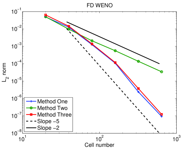
Figure 2: $L_{2}$ error norm for all three discretizations for the scalar advection problem.

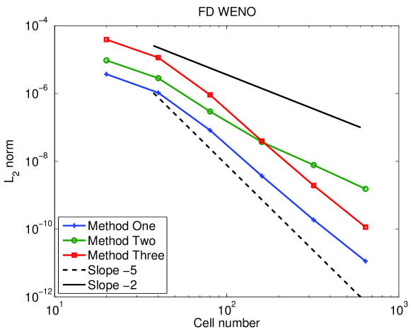
Figure 3: $L_{2}$ error norm in density for each discretization for the acoustics problem.

4.2 Euler equations: acoustics problem

A smooth problem is used to verify convergence with the Euler equations. The acoustics problem from Johnsen & Colonius [9] is adapted to spherical coordinates, with initial conditions:

$$\rho(r,0)= 1+\varepsilon f(r),$$ (14a)

$$u(r,0)= 0,$$ (14b)

$$p(r,0)= 1/\gamma+\varepsilon f(r),$$ (14c)

with perturbation

$$f(r)=\begin{cases}\frac{\sin^{4}(\pi r)}{r},&\text{ if }0.4\leq r\leq 0.6,\\ 0,&\mbox{otherwise}.\end{cases}$$ (15)

For a sufficiently small $\varepsilon$ (here $10^{-4}$), the solution remains very smooth. In this problem, the initial perturbation splits into two acoustic waves traveling in opposite directions. To prevent the singularity at the origin and boundary effects, the final time is set such that the wave has not yet reached the origin. Again, grids with $N=$ 21, 41, 81, 161, 321 and 641 are used with constant $\Delta r$. Although an exact solution to order $\varepsilon^{2}$ is known, the solution on the finest grid is used as the reference to evaluate the error.

Fig. 3 shows the $L_{2}$ error in density for this problem. The results show that Methods One and Three remain high-order and in fact fall on top of each other, although the rate now is closer to fourth order. Again, for Method Two, the rate is second order, as expected.

4.3 Sod shock tube

We consider the Sod shock tube problem [19] in cylindrical coordinate with azimuthal symmetry. The initial conditions are:

$$\left(\begin{array}[]{c}\rho\\ u\\ p\end{array}\right)_{L}=\left(\begin{array}[]{c}1\\ 0\\ 1\end{array}\right),\qquad\left(\begin{array}[]{c}\rho\\ u\\ p\end{array}\right)_{R}=\left(\begin{array}[]{c}0.125\\ 0\\ 0.1\end{array}\right).$$ (16)

The domain size is 1 and 100 equally spaced grid points are used. The location of the “diaphragm” separating the left and right states is $r=0.5$. Since no wave reaches the boundaries over the duration of the simulation (final time: $t_{f}=0.2$), the boundary scheme is irrelevant.

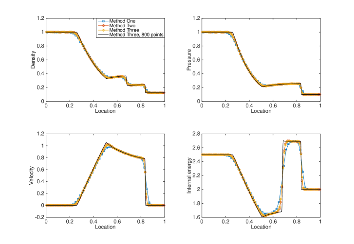
Figure 4: Profiles at $t=0.2$ for the Sod problem with 100 points.

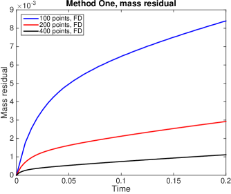
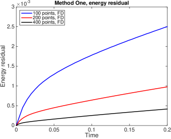
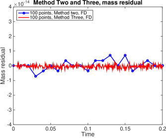
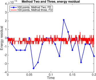
Figure 5: Mass and energy residuals vs. time for the Sod problem.

Fig. 4 shows density, velocity, pressure and internal energy profiles for this problem at the final time. Method Three on a gird of 800 points is used as a reference solution. On this grid, all three methods produce similar profiles. However, the residuals of the total mass and energy,

$$\Delta=\int_{I}\phi(t,r)dv-\int_{I}\phi(0,r)dv,$$ (17)

yield different results, as observed in Fig. 5. For FD WENO, a high-order Gauss quadrature is employed to integrate the total mass and total energy from the cell-centered values. As shown in Fig. 5, while Methods Two and Three are conservative to round-off level, Method One is not discretely conservative, as expected. In Fig. 4, differences in shock position due to lack of conservation are not clear. The total momentum is zero based on the azimuthally symmetric setup.

4.4 Sedov point-blast

Finally, we consider the Sedov point-blast problem in spherical coordinates. Following the set-up of Fryxell et al. [6] the initial conditions are

$$\left(\begin{array}[]{c}\rho\\ u\\ p\end{array}\right)=\left(\begin{array}[]{c}1\\ 0\\ 1\end{array}\right),$$ (18)

except for a few computational cells around the origin, whose pressure is

$$p_{0}^{{}^{\prime}}=\frac{3(\gamma-1)\varepsilon}{(\alpha+2)\pi\delta r^{\alpha+1}}.$$ (19)

Here, $\varepsilon=0.44$ is the dimensionless energy per unit volume. $\gamma$ is the specific heats ratioand and $\alpha$ a geometrical parameter, which is consistent with the value in Section 2. The domain size is 1, and $N=100$ with uniform spacing. We choose a constant $\delta r$ to be three times as large as the cell size for $N=100$. Reflecting boundary conditions [15] are used along the centerline; since the shock does not leave the domain, the outflow boundary scheme is irrelevant. Due to the reflecting boundary condition at the center, the high pressure region is made up of 6 cells, i.e., 3 ghost cells and 3 cells in the interior. The solution is plotted at $t=1$.

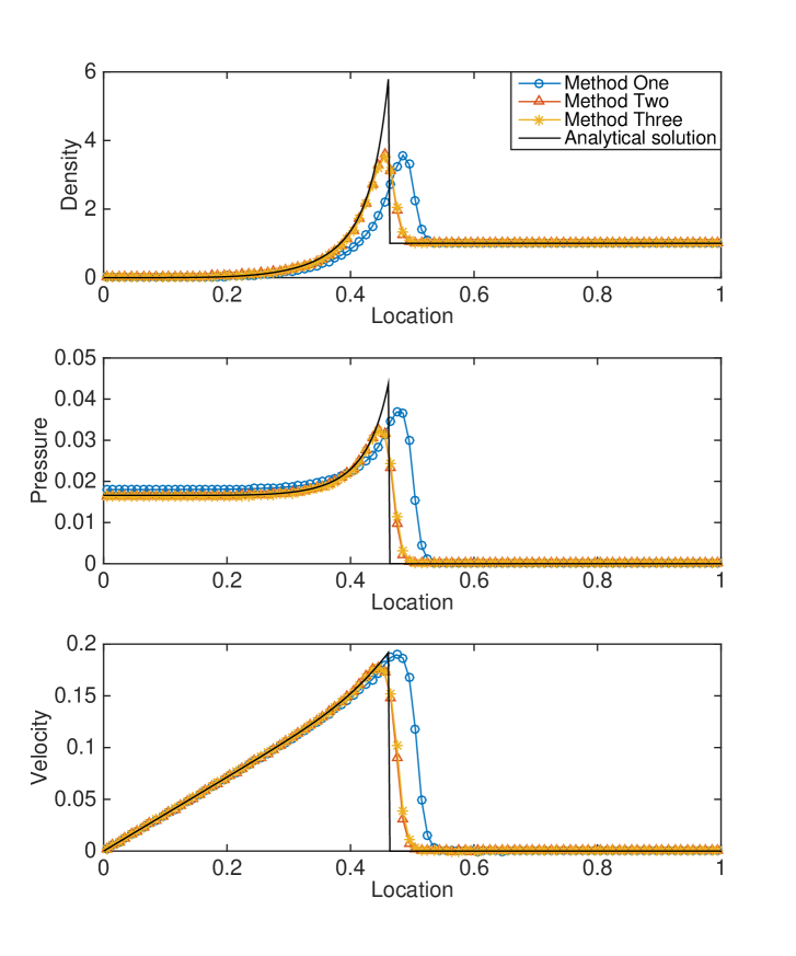
Figure 6: Profiles at $t=1$ for the Sedov problem with 100 points, FD WENO.

Density, velocity, and pressure profiles for FD WENO and the analytical solution are shown in Fig. 6. Because the total energy residual shows results qualitatively similar to the total mass residual, only the latter is shown. The density profile and mass residual for different grid size are plotted in Fig. 7. The difference in shock location is clear for this problem. Method One is non-conservative and thus produces an incorrect shock speed and thus location; it appears to converge to the correct location with grid refinement. This result is confirmed by considering the mass residual. Method Two and Three can capture the right shock position on coarse gird, whereas they need much finer grid to capture the peak of the shock. For this problem, Method Three proved to be unstable at the present Courant number due to the stiff source term, so a smaller value (0.1) is used for this problem.

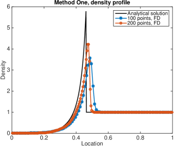
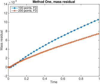
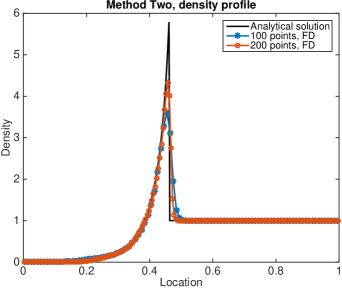
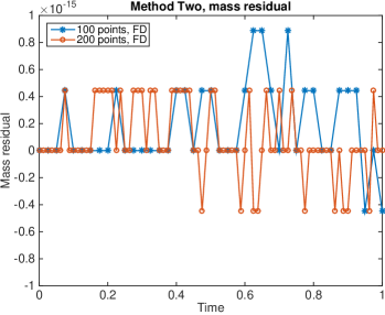
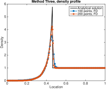
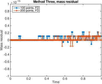
Figure 7: Density profiles and mass residuals for the Sedov problem on different grids at t = 1.

5 Conclusions

We analyzed three different spatial discretizations in cylindrical/spherical coordinates with radial dependence only for the Euler equations using finite difference WENO. In particular, high-order accuracy and conservation were evaluated. Only our newly proposed Method Three achieved high-order accuracy and was conservative. The other methods are either conservative or high-order accurate, but not both. Current work is underway to extend the analysis and implementations to discontinuous finite element methods and to incorporate diffusive effects. High-order reflecting boundary conditions will be investigated subsequently, which are not trivial for finite difference/volume schemes. This approach will form the basis for simulations of cavitation-bubble dynamics and collapse in the context of cavitation erosion.

6 Appendix

Time discretization

The classical fourth order explicit Runge-Kutta method for solving

$$u_{t}=L(u,t)$$ (20)

where is L(u, t) is a spatial discretization operator

$$u^{(1)} =u^{n}+\frac{1}{2}\Delta tL\left(u^{(n)}\right)$$ (21a)

$$u^{(2)} =u^{n}+\frac{1}{2}\Delta tL\left(u^{(1)}\right)$$ (21b)

$$u^{(3)} =u^{n}+\Delta tL\left(u^{(2)}\right)$$ (21c)

$$u^{(n+1)} =u^{n}+\frac{1}{6}\Delta t\left[L(u^{n})+2L(u^{(1)})+2L(u^{(2)})+L(u^{(3)})\right]$$ (21d)

All the numerical examples presented in this paper are obtained with this Runge-Kutta time discretization.

Local Lax-Friedrich

The flux splitting method used in this paper is the Local Lax-Friedrich splitting scheme.

$$f^{\pm}(u_{j})=\frac{1}{2}\left(f(u_{j})\pm\lambda_{j}u_{j}\right)$$ (22)

where $\lambda_{j}$ is calculated by $\lambda_{j}=\max\left|f^{{}^{\prime}}(u_{j})\right|$. Contrary to global Lax-Frederich, in which the wind speed is the maximum maximum absolute eigenvalue, the local Lax-Frederich use the maximum absolute eigenvalue at each point as the wind speed.

Implementation for the finite difference WENO scheme

A fifth order accurate finite difference WENO scheme is applied in this paper. For more details, we refer to [8].

For a scalar hyperbolic equation in 1D Cartesian coordinate

$$u_{t}+f(u)_{x}=0$$ (23)

We first consider a positive wind direction, $f^{\prime}(u)\geq 0$. For simplicity, we assume uniform mesh size $\Delta x$. A finite difference spatial discretization to approximate the derivative $f(u)_{x}$ by

$$f(u)_{x}|_{x=x_{j}}\approx\frac{1}{\Delta x}\left(\hat{f}_{j+1/2}-\hat{f}_{j-1/2}\right)$$ (24)

The numerical flux $\hat{f}_{j+1/2}$ is computed through the neighboring point values $f_{j}=f(u_{j})$. For a 5th order WENO scheme, compute 3 numerical fluxes. The three third order accurate numerical fluxes are given by

$$\hat{f}_{j+1/2}^{(1)} =\frac{1}{3}f\left(u_{j-2}\right)-\frac{7}{6}f\left(u_{j-1}\right)+\frac{11}{6}f\left(u_{j}\right)$$ (25a)

$$\hat{f}_{j+1/2}^{(2)} =-\frac{1}{6}f\left(u_{j-1}\right)+\frac{5}{6}f\left(u_{j}\right)+\frac{1}{3}f\left(u_{j+1}\right)$$ (25b)

$$\hat{f}_{j+1/2}^{(3)} =\frac{1}{3}f\left(u_{j}\right)+\frac{5}{6}f\left(u_{j+1}\right)-\frac{1}{6}f\left(u_{j+2}\right)$$ (25c)

The 5th order WENO flux is a convex combination of all these 3 numerical fluxes

$$\hat{f}_{j+1/2}=w_{1}\hat{f}_{j+1/2}^{(1)}+w_{2}\hat{f}_{j+1/2}^{(2)}+w_{3}\hat{f}_{j+1/2}^{(3)}$$ (26)

and the nonlinear weights $\omega_{i}$ are given by

$$\omega_{i}=\frac{\tilde{\omega}_{i}}{\sum_{3}^{k=1}\tilde{\omega}_{k}},\tilde{\omega}_{k}=\frac{\gamma_{k}}{\left(\epsilon+\beta_{k}\right)}$$ (27)

with the linear weights $\gamma_{k}$ given by

$$\gamma_{1}=\frac{1}{10},\gamma_{2}=\frac{3}{5},\gamma_{3}=\frac{3}{10}$$

and the smoothness indicators $\beta_{k}$ given by

$$\beta_{1} =\frac{13}{12}\left(f(u_{j-2})-2f(u_{j-1})+f(u_{j})\right)^{2}+\frac{1}{4}\left(f(u_{j-2})-4f(u_{j-1})+3f(u_{j})\right)^{2}$$ (29a)

$$\beta_{2} =\frac{13}{12}\left(f(u_{j-1})-2f(u_{j})+f(u_{j+1})\right)^{2}+\frac{1}{4}\left(f(u_{j-1})-f(u_{j+1})\right)^{2}$$ (29b)

$$\beta_{3} =\frac{13}{12}\left(f(u_{j})-2f(u_{j+1})+f(u_{j+2})\right)^{2}+\frac{1}{4}\left(3f(u_{j})-4f(u_{j+1})+f(u_{j+2})\right)^{2}$$ (29c)

where $\epsilon$ is a parameter to avoid the denominator to become 0 and is usually takes as $\epsilon=10^{-6}$ in the computation. The procedure for the case with $f^{\prime}(u)$ is mirror symmetric with respect to $i+\frac{1}{2}$.

References

- 1. Akhatov, I., Lindau,O., Topolnikov, A., Mettin, R., Vakhitova, N., Lauterborn, W., 2001. Collapse and rebound of a laser-induced cavitation bubble, Phys. Fluids. 13, 2805–2819.
- 2. Barber, B.P., Hiller, R. A., Lofstedt, R., Putterman, S. J., Weninger, K.R., 1997. Defining the Unknowns of Sonoluminescence, Phys Reports. 281, 65–143.
- 3. Bell, G. I., 1951. Taylor instability on cylinders and spheres in the small amplitude approximation, Los Alamos Scientific Laboratory, Los Alamos, NM, Report LA-1321.
- 4. Brouillette, M., 2002. The Richtmyer-Meshkov instability, Annu. Rev. Fluid Mech. 34 445–468.
- 5. De Santis, D., Geraci, G., and Guardone, A., 2014. Equivalence conditions between linear Lagrangian fniite element and node-centred finite volume schemes for conservation laws in cylindrical coordinates, Int. J. Numer. Meth. Fluids 74, 514–542.
- 6. Fryxell, B., Olson, K., Ricker, P., Timmes, F.X., Zingale, M., Lamb, D.Q., MacNeice, P., Rosner, R., Truran, J.W., Tufo, H., 2000. FLASH: An Adaptive Mesh Hydrodynamics Code for Modeling Astrophysical Thermonuclear Flashes, Astrophys. J. Suppl. Ser. 131, 273-334
- 7. Glaister, P., 1988. Flux difference splitting for the Euler equations in one spatial co-ordinate with area variation, Int. J. Numer. Meth. Fluids 8, 97–119.
- 8. Jiang, G.S., Shu, C.W., 1996. Efficient Implementation of Weighted Eno Schemes, J. Comput. Phys. 72, 78–120.
- 9. Johnsen, E., Colonius, T., 2006. Implementation of WENO schemes in compressible multicomponent problems, J. Comput. Phys. 219, 715–732.
- 10. Johnsen, E., and Colonius, T., 2008. Shock-induced collapse of a gas bubble in shockwave lithotripsy, J. Acoust. Soc. Am. 124, 2011–2020.
- 11. Johnsen, E., and Colonius, T., 2009. Numerical simulations of non-spherical bubble collapse, J. Fluid Mech. 629, 231–262.
- 12. Li, S.T., 2003. WENO Schemes for Cylindrical and Spherical Geometry, Los Alamos Report LA-UR-03-8922.
- 13. Liu, T.G., Khoo, B.C., and Yeo, K.S., 1999. The numerical simulations of explosion and implosion in air: Use of a modified Harten’s TVD scheme, Int. J. Numer. Meth. Fluids 31, 661–680.
- 14. Maire, P.H., 2009. A high-order cell-centered Lagrangian scheme for compressible fluid flows in two-dimensional cylindrical geometry, J. Comput. Phys. 228, 6882–6915.
- 15. Mohseni, K., and Colonius, T., 2000. Numerical treatment of polar coordinate singularities, J. Comput. Phys. 157, 787–795.
- 16. Omang, M., Borve, S., Trulsen, J., 2006. SPH in spherical and cylindrical coordinates, J. Comput. Phys. 212, 391–412.
- 17. Plesset, M. S., and Mitchell, T. M., 1956. On the stability of the spherical shape of a vapour cavity in a liquid, Q. Appl. Math. 13, 419–430.
- 18. Sharp, D.H., 1984. An overview of Rayleigh-Taylor Instability, Physica D. 12, 3–18
- 19. Sod, G. A., 1978. A survey of several finite difference methods for systems of nonlinear hyperbolic conservation laws, J. Comput. Phys. 27, 1–31.
- 20. Toro, E. F., 1999. Riemann solvers and numerical methods for fluid dynamics. Heidelberg, Germany: Springer-Verlag.
- 21. Vachal, P., Wendroff, B., 2014. A symmetry preserving dissipative artificial viscosity in r-z geometry, Int. J. Numer. Meth. Fluids 76, 185–198.
- 22. Von Neumann, J., Richtmyer, R.D., 1950. A Method for the Numerical Calculation of Hydrodynamic Shock. J. Appl. Phys. 21, 232–237
- 23. Wang, Z.J., Fidkowski, K., Abgrall, R., Bassi, F., Caraeni, D., Cary, A., Deconinck, H., Hartmann, R., Hillewaert, K., Huynh, H.T., Kroll, N., May, G., Persson, P.O., Van Leer, B., and Visbal, M., 2013. High-order CFD methods: current status and perspective, Int. J. Numer. Meth. Fluids 72, 811–845.
- 24. Xing, Y and Shu, C.W., 2005. High order finite difference WENO schemes with the exact conservation property for the shallow water equations, J. Comput. Phys. 208, 206-227.
- 25. Xing, Y and Shu, C.W., 2006. High order well-balanced finite difference WENO schemes for a class of hyperbolic systems with source terms, J. Sci. Comput. 27, 477-494.
- 26. Xing, Y and Shu, C.W., 2006. High order well-balanced finite volume WENO schemes and discontinuous Galerkin methods for a class of hyperbolic systems with source terms, J. Comput. Phys. 2006, 567-598.
- 27. Zhang, X.X and Shu, C.W., 2011. Positivity-preserving high order discontinuous Galerkin schemes for compressible Euler equations with source terms, J. Comput. Phys. 2011, 1238-1248.