Abstract

The paper studies derivative asset analysis in structural credit risk models where the asset value of the firm is not fully observable. It is shown that in order to determine the price dynamics of traded securities one needs to solve a stochastic filtering problem for the asset value. We transform this problem to a filtering problem for a stopped diffusion process and we apply results from the filtering literature to this problem. In this way we obtain an SPDE-characterization for the filter density. Moreover, we characterize the default intensity under incomplete information and we determine the price dynamics of traded securities. Armed with these results we study derivative asset analysis in our setup: we explain how the model can be applied to the pricing of options on traded assets and we discuss dynamic hedging and model calibration. The paper closes with a small simulation study.

Keywords.

Structural credit risk models, incomplete information, stochastic filtering, derivative asset analysis for corporate securities

1 Introduction

Structural credit risk models such as the first-passage-time models proposed by bib:black-cox-76 or bib:leland-94 are widely used in the analysis of defaultable corporate securities. In these models, a firm defaults if a random process $V$ representing the firm’s asset value hits some threshold $K$ that is typically linked to value of the firm’s liabilities. First-passage-time models offer an intuitive economic interpretation of the default event. However, in the practical application of these models a number of difficulties arise: To begin with, it might be difficult for investors in secondary markets to assess precisely the value of the firm’s assets. Moreover, for tractability reasons $V$ is frequently modelled as a diffusion process. In that case the default time $\tau$ is a predictable stopping time, which leads to unrealistically low values for short-term credit spreads. For these reasons bib:duffie-lando-01 propose a model where secondary markets have only incomplete information on the asset value $V$. More precisely they consider the situation where the market obtains at discrete time points $t_{n}$ a noisy accounting report of the form $Z_{n}=\ln V_{t_{n}}+\varepsilon_{n}$; moreover, the default history of the firm can be observed. Duffie and Lando show that in this setting the default time $\tau$ admits an intensity that is proportional to the derivative of the conditional density of the asset value at the default threshold $K$. This well-known result provides an interesting link between structural and reduced-form models. Moreover, the result shows that by introducing incomplete information it is possible to construct structural models where short-term credit spreads take reasonable values. The subsequent work of bib:frey-schmidt-09b discusses the pricing of the firm’s equity in structural models with unobservable asset value. Moreover, it is shown that the valuation of the firm’s equity and debt leads to a stochastic filtering problem: one needs to determine the conditional distribution of the current asset value $V_{t}$ given the $\sigma$-field $\mathcal{F}_{t}^{\mathcal{M}}$ representing the available information at time $t$. bib:frey-schmidt-09b consider this problem in the setup of Duffie and Lando where new information on the asset value arrives only at discrete points in time. Working with a Markov-chain approximation approximation for $V$ they derive a recursive updating rule for the conditional distribution of the approximating Markov chain via elementary Bayesian updating; the discrete nature of the information-arrival is crucial for their arguments.

Neither bib:duffie-lando-01 nor bib:frey-schmidt-09b study the price dynamics of traded securities under incomplete information. Hence in these papers it is not possible to analyze the pricing and the hedging of derivative securities such as options on corporate bonds or on the stock. The main goal of the present paper is therefore to develop a proper theory of derivative asset analysis for structural credit risk models under incomplete information.

More precisely, we make the following contributions. First, in order to obtain realistic price dynamics for the traded securities, we model the noisy observations of the asset value by a continuous time process of the form $Z_{t}=\int_{0}^{t}a(V_{s})ds+W_{t}$ for some Brownian motion $W$ independent of $V$. We show that this leads to price processes with non-zero instantaneous volatility, whereas the discrete information arrival considered by Duffie and Lando or Frey and Schmidt generates asset prices that evolve deterministically between the news-arrival dates. Moreover, modeling $Z$ as a continuous time processes is in line with the standard literature on stochastic filtering such as bib:bain-crisan-08. Second, in order to derive the price dynamics of traded securities we determine the dynamics of the conditional distribution of $V_{t}$ given $\mathcal{F}_{t}^{\mathcal{M}}$. This is a challenging stochastic filtering problem, since under full observation the default time $\tau$ is predictable, so that standard filtering techniques for point process observations (see for instance bib:bremaud-81) do not apply. We therefore transform the original problem to a new filtering problem where the observations consist only of the process $Z$; the signal process in this new problem is on the other hand given by the asset value process stopped at the first exit time of the solvency region $(K,\infty)$. Using results of bib:pardoux-78 on the filtering of stopped diffusion processes we derive a stochastic partial differential equation (SPDE) for the conditional density of $V_{t}$ given $\mathcal{F}_{t}^{\mathcal{M}}$, denoted $\pi(t,\cdot)$, and we discuss the numerical solution of this SPDE via a Galerkin approximation. Extending the work of bib:duffie-lando-01 to our more general information structure, we show that $\tau$ admits an intensity process $(\lambda_{t})_{t\geq 0}$ such that the intensity at time $t$ is proportional to the spatial derivative of $\pi(t,v)$ at $v=K$. Armed with these results we finally study derivative asset analysis in our setup: we identify the price dynamics of the traded securities; we consider the pricing of options on traded assets; we derive risk-minimizing dynamic hedging strategies for these claims, and we discuss model calibration. The paper closes with a small simulation study illustrating the theoretical results.

Incomplete information and filtering methods have been used before in the analysis of credit risk. Structural models with incomplete information were considered among others by bib:kusuoka-99, bib:duffie-lando-01, bib:jarrow-protter-04, bib:coculescu-geman-jeanblanc-06, bib:frey-schmidt-09b and bib:cetin-12. The last contribution is related to the present paper. Working in a similar setup as ours, Cetin uses probabilistic arguments to establish the existence of a default intensity with respect to $\mathbb{F}^{\mathcal{M}}$, and he derives the corresponding filter equations. He does not discuss the existence of the conditional density $\pi(t,\cdot)$ and financial applications are discussed only in a peripheral manner. From a purely mathematical point of view our paper is also closely related to bib:krylov-wang-11 who deal with the filtering of partially observed diffusions up to the first exit time of a domain. The relation between our results and those of Krylov and Wang are best explained once the mathematical details of our setup have been introduced, and we refer to Section 4, Remark 4.5 for a deeper discussion of similarities and differences between the two papers.

Reduced-form credit risk models with incomplete information have been considered previously by bib:duffie-et-al-06, bib:frey-runggaldier-10 and bib:frey-schmidt-12, among others. The modelling philosophy of the present paper is inspired by bib:frey-schmidt-12, but the mathematical analysis differs substantially. In particular, in bib:frey-schmidt-12 the default times of the firms under consideration do admit an intensity under full information. Hence the filtering problem that arises in the pricing of credit derivatives can be addressed via a straightforward application of the innovations approach to nonlinear filtering.

The remainder of the paper is organized as follows. In Section 2 we introduce the model; the relation between traded securities and stochastic filtering is discussed in Section 3; Section 4 is concerned with the stochastic filtering of the asset value; in Section 5 we derive the dynamics of corporate securities; Section 6 is concerned with derivative asset analysis; the results of numerical experiments are given in Section 7.

Acknowledgements.

Financial support from the German Science Foundation (DFG) and from the Vienna Science and Technology Fund (WWTF), project MA14-031, is gratefully acknowledged. Moreover, we thank Andreas Peterseil for very competent research assistance and several anonymous referees for useful comments.

2 The Model

We begin by introducing the mathematical structure of the model. We work on a filtered probability space $(\Omega,\mathcal{G},\mathbb{G}=(\mathcal{G}_{t})_{t\geq 0},Q)$ and we assume that all processes introduced below are $\mathbb{G}$-adapted. Since we are mainly interested in the pricing of derivative securities we assume that $Q$ is the risk-neutral pricing measure. We consider a company with nonnegative asset value process $V=(V_{t})_{t\geq 0}$. The company is subject to default risk and the default time is modelled as a first passage time, that is

$$\tau=\inf\{t\geq 0\colon V_{t}\leq K\}$$ (2.1)

for some default threshold $K>0$. In practice $K$ might represent solvency capital requirements imposed by regulators (see Example 2.3) or it might correspond to an endogenous default threshold as in bib:duffie-lando-01 (see Example 2.4). By $Y_{t}=1_{\{\tau\leq t\}}$ we denote the default state of the firm at time $t$, that is $Y_{t}=1$ if and only if the firm has defaulted by time $t$; the associated default indicator process is denoted by $Y=(Y_{t})_{t\geq 0}$.

Assumption 2.1 (Dividends and asset value process).

1) The risk free rate of interest is constant and equal to $r\geq 0$.

2) The firm pays dividends at equidistant deterministic time points $t_{1}$, $t_{2},\ldots$ (for instance semi-annual dividend payments). The set of dividend dates is denoted by $\mathcal{T}^{D}$. The dividend payment at $t_{n}$ is a random percentage of the surplus $(V_{t_{n}-}-K)^{+}$ (the part of the asset value that can be distributed to shareholders without sending the company into immediate default). Denoting by $d_{n}$ the dividend payment at $t_{n}$, it holds that

$$d_{n}=\delta_{n}(V_{t_{n}}-K)^{+};$$ (2.2)

here $(\delta_{n})_{n=1,2,\dots}$ is an iid sequence of noise variable that are independent of $V$, take values in $(0,1)$ and that have density function $\varphi_{\delta}$. We assume that $\varphi_{\delta}$ is bounded and twice continuously differentiable on $[0,1]$ with $\varphi_{\delta}(1)=0$. For $V_{t_{n}-}>K$ the conditional distribution of $d_{n}$ given the history of the asset value process is thus of the form $\varphi(y,V_{t_{n}-})dy$ where

$$\varphi(y,v)=\frac{1}{(v-K)}\varphi_{\delta}\Big{(}\frac{y}{(v-K)}\Big{)}1_{\{v>K\}}\,.$$ (2.3)

Let $D_{t}=\sum_{\{n\colon t_{n}\leq t\}}d_{n}$ so that $D=(D_{t})_{t\geq 0}$ is the cumulative dividend process. In the sequel we denote by $\mu^{D}(dy,dt)$ the random measure associated with the sequence $(t_{n},d_{n})_{n\in\mathbb{N}}$.

3) The asset value process $V=(V_{t})_{t\geq 0}$ has the following dynamics

$$V_{t}=V_{0}+\int_{0}^{t}rV_{s}ds+\int_{0}^{t}\sigma V_{s}dB_{s}-\kappa D_{t}$$ (2.4)

for a constant volatility $\sigma>0$, a standard $Q$-Brownian motion $B$ and a random variable $V_{0}$. The parameter $\kappa$ takes values in $\{0,1\}$. For $\kappa=1$ (the most relevant case) the asset value is reduced at a dividend date by the amount $d_{n}$ distributed to shareholders; $\kappa=0$ corresponds to the case where we view the $d_{n}$ merely as noisy signal of the asset value and not as a payment to shareholders (see Example 2.4). We assume that $V_{0}$ has Lebesgue density $\pi_{0}(v)$ for a continuously differentiable function $\pi_{0}\colon[K,\infty)\to\mathbb{R}^{+}$ with $\pi_{0}(K)=0$ such that $V_{0}$ has finite second moment.

The second assumption reflects the fact that in reality there is a positive but noisy relation between asset value and dividend size. Note that it follows from (2.3) that $d_{n}<(V_{t_{n}-}-K)^{+}$. This restriction on the dividend size can be viewed as implicit protection of debtholders as it ensures that the firm will not default at a dividend date due to an overly large dividend. Together with our assumptions on $\varphi_{\delta}$, (2.3) implies that for a given $d>0$, $\varphi(d,v)$ is zero for all $v$ such that $d/(v-K)\geq 1$, that is for $v\leq d+K$. Moreover, it holds that

$$\sup_{v\geq K}\varphi(d,v)\leq\frac{1}{d}\max_{\delta\in[0,1]}\varphi_{\delta}(\delta)\,.$$ (2.5)

Note that the dividend policy (2.2) is not the outcome of a formal optimization process. In fact, as shown for instance in bib:jeanblanc-shiriayev-95, it might be optimal to pay out a larger fraction of the available surplus if $V_{t_{n}}$ is large. While the filtering results in Section 4.3 could be extended to such a setup, provided the conditional density $\varphi(\cdot,v)$ of the dividend size satisfies certain regularity conditions, the pricing of the firm’s stock would become more involved. Moreover, dividend policies adopted in practice are guided to a large extent by market conventions and rules of thumb. For these reasons we stick to the simple rule (2.2).

The $\mathbb{G}$-compensator of the random measure $\mu^{D}$ associated with the sequence $(t_{n},d_{n})_{n\in\mathbb{N}}$ is given by $\gamma^{D}(dy,dt)=\sum_{n=1}^{\infty}\varphi(y,V_{t_{n}-})dy\,\delta_{\{t_{n}\}}(dt)$. Note that for $g\colon[0,\infty)\times[0,\infty)\to\mathbb{R}^{+}$ it holds that

$$\int_{0}^{\infty}\int_{0}^{\infty}g(t,y)\gamma^{D}(dy,dt)=\sum_{n=1}^{\infty}\int_{0}^{\infty}g(t_{n},y)\varphi(y,V_{t_{n}-})dy\,.$$

The assumption that between dividends the asset value is a geometric Brownian motion is routinely made in the literature on structural credit risk models such as bib:leland-94 or bib:duffie-lando-01. For empirical support for the assumption of geometric Brownian motion as a model for the asset price dynamics we refer to bib:moodys-edf-12. Note that the assumption that $V$ follows a geometric Brownian motion does not imply that the stock price follows a geometric Brownian motion. In fact, our analysis in Section 5 shows that in our setup the stock price dynamics can be much ‘wilder’ than geometric Brownian motion. Note finally that $V$ is not a traded asset so that its drift under $Q$ might in principle be different from the risk-free rate $r$. However, setting the drift of $V$ equal to $r$ permits us to interpret $V$ as value of all future dividend payments of the firm (up to $t=\infty$), see Lemma 3.2 below.

Information structure and pricing.

In our setting the asset value $V$ is not directly observable. Instead we assume that prices of corporate securities are determined as conditional expectation with respect to some filtration $\mathbb{F}^{\mathcal{M}}=(\mathcal{F}_{t}^{\mathcal{M}})_{t\geq 0}$ that is generated by the default history, by the dividend payments of the firm and by observations of functions of $V$ in additive Gaussian noise:

Assumption 2.2.

It holds that $\mathbb{F}^{\mathcal{M}}=\mathbb{F}^{Y}\vee\mathbb{F}^{D}\vee\mathbb{F}^{Z}$, where $\mathbb{F}^{Y}$ denotes the filtration generated by the default indicator process $Y$, where $\mathbb{F}^{D}$ denotes the filtration generated by $D$ and where the filtration $\mathbb{F}^{Z}$ is generated by the $l$-dimensional process $Z$ with

$${Z}_{t}=\int_{0}^{t}{a}(V_{s})ds+{W}_{t}\,.$$ (2.6)

Here ${W}$ is an $l$-dimensional $\mathbb{G}$-Brownian motion independent of $B$, and $a=(a^{1},\dots,a^{l})$ is a bounded and continuously differentiable function from $\mathbb{R^{+}}$ to $\mathbb{R}^{l}$ with $a(K)=0$. Note that the assumption $a(K)=0$ is no real restriction as the function $a$ can be replaced with $a-a(K)$ without altering the information content of $\mathbb{F}^{\mathcal{M}}$.

In the sequel $\mathbb{F}^{\mathcal{M}}$ is called modeling filtration, since it represents the fictitious flow of information that is employed in the construction of the model. In particular, we will not associate the process $Z$ with publicly observable economic data; it is simply a mathematical device that generates the diffusive component in the asset price dynamics. As explained in the next section, for the application of the model, that is for pricing and hedging of derivative securities, it is sufficient to observe the price processes of traded assets and the default history of the firm. This is important since pricing formulas and hedging strategies need to be computed in terms of publicly available information.

We use martingale modelling to construct the price processes of traded securities and we define the ex-dividend price of a generic traded security with $\mathbb{F}^{\mathcal{M}}$-adapted cash flow stream $(H_{t})_{0\leq t\leq T}$ and maturity date $T\in(0,\infty]$ by

$$\Pi_{t}^{H}=E^{Q}\Big{(}\int_{t}^{T}e^{-r(s-t)}dH_{s}\mid\mathcal{F}_{t}^{\mathcal{M}}\Big{)}\,,\quad t\leq T,$$ (2.7)

provided of course that the discounted cash flow stream is $Q$ integrable. The use of the risk-neutral pricing formula (2.7) ensures that the discounted gains from trade of every traded security are martingales, which is sufficient to exclude arbitrage opportunities. Hedging arguments within the martingale modelling paradigm are presented in Section 6.2.

Finally we describe two economic settings that can be embedded in our framework.

Example 2.3.

Our first example is that of a financial institution that is subject to financial regulation. We assume that the institution has issued shares to outside shareholders. It is run by a management team that knows the asset value $V$. Management is prevented from actively trading the shares of the institution, for instance because of insider trading regulation. Outside stock and bond investors on the other hand are unable to discern the exact asset value from public information. The dividend policy of the firm is of the form (2.2). In this example we let $\kappa=1$ so that dividend payments do reduce the asset value of the firm. We assume that the institution is subject to capital adequacy rules such as the Basel III or the Solvency II rules. Loosely speaking these rules require that the ratio of the equity capital of the firm over its total asset value must be larger than a given threshold $\gamma\in(0,1)$. If we denote by $\tilde{K}$ the value of the firms liabilities, this translates into the condition that $(V_{t}-\tilde{K})/V_{t}>\gamma$ and hence that

$$V_{t}>K:=\tilde{K}/(1-\gamma).$$ (2.8)

We assume that regulators actively monitor that the state of the firm is in accordance with the capital adequacy rule (2.8) and that management provides them with correct information about the asset value. If $V$ falls below $K$, regulators shut down the financial institution and there is a default. Hence the default time is a first passage time with default threshold $K$ given in (2.8). Note that in this setting default is enforced by regulators with privileged access to information.

Example 2.4.

The well-known model of bib:duffie-lando-01 can be embedded in our setup as well. Duffie and Lando consider a firm that is operated by risk-neutral equity owners who have complete information about $V$. The firm issues some debt in the form of a consol bond in order to profit from the tax shield of debt, but there are no traded shares and no dividend payments to outside investors. Equity owners are prohibited from trading in bond markets by insider trading regulation. In this setup the owners of the firm have the option to stop servicing the firm’s debt, in which case the firm defaults. Following bib:leland-toft-96, Duffie and Lando show that the optimal default time (for the equity owners) is a first passage time, but now with endogenously determined default threshold $K$.

Note that in this example the random variables $d_{n}$ can be viewed as additional information on $V$ that arrives at discrete time points, such as earnings announcements. This interpretation corresponds to a value of $\kappa=0$ for the parameter $\kappa$ in (2.4). Moreover, the rvs $d_{n}$ do not have to be of the special form (2.2); it suffices that for fixed $d$ the mapping $v\mapsto\varphi(d,v)$ is smooth and bounded.

3 Prices of Traded Securities and Stochastic Filtering

In this section we explain the relation between the prices of traded securities and stochastic filtering and we discuss several examples.

Traded securities.

The set of traded securities consists so-called basic debt securities and of the stock of the firm. We now describe the payoff stream of these securities in more detail. First we refer to an asset as a basic debt security if its cash-flow stream can be expressed as a linear combination of the following two building blocks

• A survival claim with generic maturity date $T$. This claim pays one unit of account at $T$, provided that $\tau>T$.

• A payment-at-default claim with generic maturity date $T$. This claim pays one unit directly at $\tau$, provided that $\tau\leq T$.

It is well known that bonds issued by the firm and credit default swaps on the firm can be expressed as linear combination of these building blocks, see for instance bib:Lando-98.

Next we discuss the modelling of the firm’s stock. The shareholders of the firm receive the dividend payments made by the firm at dividend dates $t_{n}<\tau$. Hence the cumulative cashflow stream received by the shareholders up to time $t$ equals $H_{t}^{\text{stock}}=D_{t\wedge\tau}$. The risk neutral pricing formula (2.7) thus implies that the value of the firm’s stock is given by

$$S_{t}=E^{Q}\Big{(}\sum_{\{n\colon t_{n}>t\}}1_{\{\tau>t_{n}\}}e^{-(t_{n}-t)}d_{n}\mid\mathcal{F}_{t}^{\mathcal{M}}\Big{)}\,.$$ (3.1)

Note that the cash-flow stream of a basic debt security and of the stock is adapted to $\mathbb{F}^{Y}\vee\mathbb{F}^{D}$ and hence also to the modelling filtration $\mathbb{F}^{\mathcal{M}}$.

Relation to stochastic filtering.

Consider now a traded security with cash-flow stream $(H_{t})_{0\leq t\leq T}$ and ex-dividend price $\Pi_{t}^{H}=E^{Q}\big{(}\int_{t}^{T}e^{-r(s-t)}dH_{s}\mid\mathcal{F}_{t}^{\mathcal{M}}\big{)}$. In the sequel we mostly consider the pre-default value of the security given by $1_{\{\tau>t\}}\Pi_{t}^{H}$ (pricing for $\tau\leq t$ is largely related to the modelling of recovery rates which is of no concern to us here). Using iterated conditional expectations we get that

$$1_{\{\tau>t\}}\Pi_{t}^{H}=E^{Q}\Big{(}E^{Q}\big{(}1_{\{\tau>t\}}\int_{t}^{T}e^{-r(s-t)}dH_{s}\mid\mathcal{G}_{t}\big{)}\mid\mathcal{F}_{t}^{\mathcal{M}}\Big{)}.$$ (3.2)

By the Markov property of $V$, for basic debt securities and for the stock the inner conditional expectation can be expressed as a function of time and of the current asset value $V_{t}$, that is

$$E^{Q}\Big{(}1_{\{\tau>t\}}\int_{t}^{T}e^{-r(s-t)}dH_{s}\mid\mathcal{G}_{t}\Big{)}=1_{\{\tau>t\}}h(t,V_{t})\,.$$ (3.3)

The function $h$ is called the full-information value of the security. In Section 4 we show that on the $\mathcal{F}_{t}^{\mathcal{M}}$-measurable set $\{\tau>t\}$ the conditional distribution of $V_{t}$ given $\mathcal{F}_{t}^{\mathcal{M}}$ admits a density $\pi(t,\cdot)\colon[K,\infty)\to\mathbb{R}^{+}$ and we derive an SPDE for this density. Substituting (3.3) into (3.2) gives that

$$1_{\{\tau>t\}}\Pi_{t}^{H}=1_{\{\tau>t\}}E^{Q}\big{(}h(t,V_{t})\mid\mathcal{F}_{t}^{\mathcal{M}})=1_{\{\tau>t\}}\int_{K}^{\infty}h(t,v)\pi(t,v)dv\,.$$ (3.4)

Relation (3.4) provides an important relationship between prices of traded securities and stochastic filtering, which is used in two ways. First, at any given time point $t_{0}$ an estimate of $\pi(t_{0})$ is backed out from the price of traded securities at time $t_{0}$, so that $\pi(t_{0})$ can be viewed as a function of observed prices (the necessary calibration methodology is described in Section 6.3). Moreover, in Section 6.1 we show that the price at time $t_{0}$ of an option on the traded assets is a function of $\pi(t_{0})$. Hence option prices can be evaluated using observable quantities (prices of traded securities) as input. Second, in order to derive the price dynamics of traded securities under the risk-neutral measure $Q$ we determine the dynamics of $\pi(t)$ using filtering methods; using (3.4) this gives the dynamics of the pre-default value $1_{\{\tau>t\}}\Pi_{t}^{H}$ of the traded securities.

This approach is akin to the use of factor models in term structure modelling where prices of traded securities are used to estimate the current value of the factor process and where bond price dynamics are derived from the dynamics of the factor process. In fact, our model can be viewed as factor model with infinite-dimensional factor process $\pi(t)$.

Remark 3.1.

Our modelling strategy leads to filtering problems under $Q$ and differs from the ‘classical’ application of stochastic filtering in statistical inference. A typical problem in the latter context would be as follows: the process $Z$ is identified with a specific set of economic data that contains noisy information of $V$, and filtering techniques are employed to estimate the conditional distribution of $V_{t}$ under the historical measure $P$ given the observed trajectories of $Z$, $D$ and $Y$ up to time $t$. Such an approach could be used to estimate the firm’s real-world default probability, similar in spirit to the well-known public firm EDF model bib:moodys-edf-12. It is worth mentioning that the mathematical results developed in Sections 4 and 5 cover also applications of this type.

Full information value of traded securities.

Next we discuss the computation of the full information value $h$ for basic debt securities and for the stock. We concentrate on the case $\kappa=1$, so that there is a downward jump in $V$ at the dividend dates; for $\kappa=0$ the asset value is a geometric Brownian motion and the ensuing computations are fairly standard.

We begin with a survival claim with payoff $H_{T}=1_{\{\tau>T\}}$ and associated full-information value $h^{\text{surv}}(t,V_{t})$. Since $e^{-rt}h^{\text{surv}}(t,V_{t})$ is a $\mathbb{G}$-martingale we get the following PDE characterization of $h^{\text{surv}}$: first, between dividend dates $h^{\text{surv}}$ solves the boundary value problem $\frac{d}{dt}h^{\text{surv}}+\mathcal{L}h^{\text{surv}}=rh^{\text{surv}}$ with boundary condition $h^{\text{surv}}(t,K)=0$ for $0\leq t\leq T$, where we let for $f\in\mathcal{C}^{2}(0,\infty)$

$$\mathcal{L}f(v)=rv\frac{df(v)}{dv}+\frac{1}{2}\sigma^{2}v^{2}\frac{d^{2}f(v)}{dv^{2}}\,;$$ (3.5)

second, at a dividend date $t_{n}\leq T$ it holds that

$$h^{\text{surv}}(t_{n}-,v)=\int_{0}^{v-K}h^{\text{surv}}(t_{n},v-y)\varphi(y,v)dy\,;$$ (3.6)

finally, one has the terminal condition $h^{\text{surv}}(T,v)=1$ for $v>K$. These conditions can be used to compute $h^{\text{surv}}$ numerically by a backward induction over the dividend dates; see for instance bib:vellekoop-nieuwenhuis-06 for details. Moreover, we will need the PDE characterization of $h^{\text{surv}}$ to derive the price dynamics of a survival claim under incomplete information in Section 5.2. Recall that a payment-at-default claim with maturity $T$ pays one unit directly at $\tau$, provided that $\tau\leq T$. The PDE characterization is similar to the case of a survival claim; however, now the boundary condition is $h^{\text{def}}(t,K)=1$, $0\leq t\leq T$ and the terminal value is $h^{\text{def}}(T,v)=0$, $v>K$. By definition the full information value of all basic debt securities can be computed from $h^{\text{surv}}$ and $h^{\text{def}}$.

Next we consider the stock of the firm. It follows from (3.1) that the full information value of the firm’s stock is given by

$$h^{\text{stock}}(t,v)=E^{Q}\Big{(}\sum_{n\colon t_{n}>t}1_{\{\tau>t_{n}\}}e^{-r(t_{n}-t)}d_{n}\mid V_{t}=v\Big{)}$$ (3.7)

The next lemma whose proof is given in Appendix B shows that $V_{t}$ can be interpreted as value of all future dividend payments (up to $T=\infty$).

Lemma 3.2.

Under Assumption 2.1 it holds that $E^{Q}\big{(}\sum_{t_{n}\geq t}e^{-r(t_{n}-t)}d_{n}\mid V_{t}\big{)}=V_{t}$.

Note that Lemma 3.2 implies that $h^{\text{stock}}(t,v)<v$. It follows that the stock price $S_{t}$ is finite as well (this is not a priori clear since $S_{t}$ is the expected value of an infinite payment stream). Using the fact that $e^{-rt}h^{\text{stock}}(t,V_{t})+\int_{0}^{t}1_{\{\tau>s\}}e^{-rs}dD_{s}$ is a $Q$ martingale we obtain the following PDE characterization for $h^{\text{stock}}$: between dividend dates $h^{\text{stock}}$ solves the PDE $\frac{d}{dt}h^{\text{stock}}+\mathcal{L}h^{\text{stock}}=rh^{\text{stock}}$ with boundary condition $h^{\text{stock}}(t,K)=0$; at the dividend date $t_{n}$ $h^{\text{stock}}$ satisfies the relation

$$h^{\text{stock}}(t_{n}-,v)=\int_{0}^{v-K}\left(h^{\text{stock}}(t_{n},v-y)+y\right)\varphi(y,v)dy\,.$$ (3.8)

Since we assumed equidistant dividend dates it holds that $h^{\text{stock}}(t,v)=h^{\text{stock}}(t+\Delta t,v)$ for $\Delta t=t_{n}-t_{n-1}$ so that it is enough to compute $h^{\text{stock}}(t,v)$ for $0\leq t\leq t_{1}$. An explicit formula for $h^{\text{stock}}$ is not available; the main problem is the fact that the downward jump in $V$ at a dividend date combines arithmetic and geometric expressions. There are essentially two options for computing $h^{\text{stock}}$ numerically. On the one hand one can rely on Monte Carlo methods. In order to speed up the simulation explicit pricing formulas for $h^{\text{stock}}$ in a Black Scholes model with continuous dividend stream can be used as control variate. Alternatively, it is possible to use PDE methods in order to compute $h^{\text{stock}}$. We omit the details since the numerical computation of option prices is not central to our analysis.

4 Stochastic Filtering of the Asset Value

Fix some horizon date $T$, for instance the largest maturity date of all outstanding derivative securities related to the firm. Recall from the previous section that in order to derive the price dynamics of traded securities we need to determine the dynamics of the conditional density $\pi(t)$, $0\leq t<\tau\wedge T$. This problem is studied in the present section.

4.1 Preliminaries

Following the usual approach in stochastic filtering we start with a characterization of the conditional distribution of $V_{t}$ given $\mathcal{F}_{t}^{\mathcal{M}}$ (the filter distribution) in weak form. More precisely, given a function $h$ on $[K,\infty)$ such that $E\big{(}|h(V_{t})|\big{)}<\infty$ for all $t\leq T$ we want to derive the dynamics of the conditional expectation

$$1_{\{\tau>t\}}E^{Q}\big{(}h(V_{t})\mid\mathcal{F}_{t}^{\mathcal{M}}\big{)},\quad t\leq T\,.$$ (4.1)

This is sufficient for our purposes since we are only interested in the dynamics of the filter distribution prior to default.

The problem (4.1) is a challenging filtering problem since the default time $\tau$ does not admit an intensity under full information. Hence standard filtering techniques for point process observations as in bib:bremaud-81 do not apply. This issue is addressed in the following proposition where, loosely speaking, (4.1) is transformed to a filtering problem with respect to the background filtration $\mathbb{F}^{Z}\vee\mathbb{F}^{D}$.

Proposition 4.1.

Denote by $V^{\tau}=(V_{t\wedge\tau})_{t\geq 0}$ the asset value process stopped at the default boundary, by $\tilde{Z}_{t}=\int_{0}^{t}a(V_{s}^{\tau})ds+W_{t}$ the observation of $V^{\tau}$ in additive Gaussian noise and by $\tilde{D}_{t}=\sum_{\{n\colon t_{n}\leq t\}}\delta_{n}(V_{t_{n}-}^{\tau}-K)^{+}$ the cumulative dividend process corresponding to $V^{\tau}$. Then we have for $h:[K,\infty)\to\mathbb{R}$ such that $E^{Q}\big{(}|h(V_{t})|\big{)}<\infty$ for all $t\leq T$

$$1_{\{\tau>t\}}E^{Q}(h(V_{t})\mid\mathcal{F}_{t}^{\mathcal{M}})=1_{\{\tau>t\}}\frac{E^{Q}\big{(}h(V_{t}^{\tau})1_{\{V_{t}^{\tau}>K\}}\mid\mathcal{F}_{t}^{\tilde{Z}}\vee\mathcal{F}_{t}^{\tilde{D}}\big{)}}{Q\big{(}V_{t}^{\tau}>K\mid\mathcal{F}_{t}^{\tilde{Z}}\vee\mathcal{F}_{t}^{\tilde{D}}\big{)}}\,.$$ (4.2)

Proof.

For notational simplicity we ignore the dividend observation in the proof so that $\mathbb{F}^{\mathcal{M}}=\mathbb{F}^{Z}\vee\mathbb{F}^{Y}$. The first step is to show that

$$E^{Q}\big{(}h(V_{t})1_{\{\tau>t\}}\mid\mathcal{F}_{t}^{\mathcal{M}}\big{)}=E^{Q}\big{(}h(V_{t}^{\tau})1_{\{\tau>t\}}\mid\mathcal{F}_{t}^{\tilde{Z}}\vee\mathcal{F}_{t}^{Y}\big{)}\,,$$ (4.3)

where the filtration $\mathbb{F}^{\tilde{Z}}$ is generated by the noisy observations of the stopped asset value process; the proof of this identity is given in Appendix B.

Second, using the Dellacherie formula (see for instance Lemma 3.1 in bib:elliott-jeanblanc-yor-00) and the relation $\{\tau>t\}=\{V_{t}^{\tau}>K\}$, we get

$$E^{Q}\big{(}h(V_{t}^{\tau})1_{\{\tau>t\}}\mid\mathcal{F}_{t}^{\tilde{Z}}\vee\mathcal{F}_{t}^{Y}\big{)} =1_{\{\tau>t\}}\frac{E^{Q}\big{(}h(V_{t}^{\tau})1_{\{\tau>t\}}\mid\mathcal{F}_{t}^{\tilde{Z}}\big{)}}{Q\big{(}\tau>t\mid\mathcal{F}_{t}^{\tilde{Z}}\big{)}}$$

$$=1_{\{\tau>t\}}\frac{E^{Q}\big{(}h(V_{t}^{\tau})1_{\{V_{t}^{\tau}>K\}}\mid\mathcal{F}_{t}^{\tilde{Z}}\big{)}}{Q\big{(}V_{t}^{\tau}>K\mid\mathcal{F}_{t}^{\tilde{Z}}\big{)}}\,,$$

as claimed. ∎

With the notation $f(v):=h(v)1_{\{v>K\}}$, Proposition 4.1 shows that in order to evaluate the right side of (4.2) one needs to compute for generic $f:[K,\infty)\to\mathbb{R}$ such that $E^{Q}\big{(}|f(V_{t}^{\tau})|\big{)}<\infty$ for all $0\leq t\leq T$ conditional expectations of the form

$$E^{Q}\big{(}f(V_{t}^{\tau})\mid\mathcal{F}_{t}^{\tilde{Z}}\vee\mathcal{F}_{t}^{\tilde{D}}\big{)}\,.$$ (4.4)

This is a stochastic filtering problem with signal process given by $V^{\tau}$ (the asset value process stopped at the first exit time of the halfspace $(K,\infty)$). In the sequel we study this problem using results of bib:pardoux-78 on the filtering of diffusions stopped at the first exit time of some bounded domain, first for the case without dividends and in Section 4.3 for the general case. In order to apply the results of bib:pardoux-78 we fix some large number $N$ and replace the unbounded halfspace $(K,\infty)$ with the bounded domain $(K,N)$. For this we define the stopping time $\sigma_{N}=\inf\{t\geq 0\colon V_{t}\geq N\}$ and we replace the original asset value process $V$ with the stopped process $V^{N}:=(V_{t\wedge\sigma_{N}})_{t\geq 0}$. Applying Proposition 4.1 to the process $V^{N}$ leads to a filtering problem with signal process $X:=(V^{N})^{\tau}$. More precisely, one has to compute conditional expectations of the form

$$E^{Q}\big{(}f(X_{t})\mid\mathcal{F}_{t}^{Z^{N}}\vee\mathcal{F}_{t}^{D^{N}}\big{)}$$ (4.5)

where, with a slight abuse of notation, ${Z}_{t}=\int_{0}^{t}{a}(X_{s})ds+{W}_{t}$ and $D_{t}=\sum_{t_{n}\leq t}\delta_{n}(X_{t_{n}-}-K)^{+}.$ Note that $\tau\wedge\sigma_{N}$ is the first exit time of $V$ from the domain $(K,N)$. Moreover, it holds by definition that $X_{t}=V_{t\wedge\tau\wedge\sigma_{N}}$, i.e. $X$ is equal to the asset value process $V$ stopped at the boundary of the bounded domain $(K,N)$. Hence the state space of $X$ is given by $S^{X}:=[K,N]$ and the analysis of bib:pardoux-78 applies to the problem (4.5).

In the next proposition we show that the reduction to a bounded domain $(K,N)$, that is the use of the stopped process $V^{N}$ as underlying asset value process instead of the original process $V$, does not affect the financial implications of the analysis, provided that $N$ is sufficiently large. In order to state the result we need to make the dependence of the model quantities on $N$ explicit: Let ${Z}_{t}^{N}=\int_{0}^{t}{a}(V_{s}^{N})ds+{W}_{t}$, $D_{t}=\sum_{\{n\colon t_{n}\leq t\}}\delta_{n}(V^{N}_{t_{n}-}-K)^{+}$ and $\tau^{N}=\inf\{t\geq 0\colon V_{t}^{N}\leq K\}$, and denote by $\mathbb{F}^{\mathcal{M},N}$ the modelling filtration in the model with asset value $V^{N}$, that is the filtration generated by $Z^{N}$, $D^{N}$ and by the default indicator $1_{\{\tau^{N}\leq t\}}$.

Proposition 4.2.

1. Fix some horizon date $T>0$ and let $\mathbb{F}$ be an arbitrary subfiltration of $\mathbb{G}$. Then for $\epsilon>0$, it holds that

$$Q\Big{(}\sup_{0\leq t\leq T}Q(\sigma_{N}\leq t\mid\mathcal{F}_{t})>\epsilon\Big{)}\leq\frac{1}{\epsilon}Q(\sigma_{N}\leq T)\to 0\text{ as $N\to\infty$}.$$

2. The price process of the traded securities in the model with asset value process $V^{N}$ converges in ucp (uniformly on compacts in probability) to the price process in the model with asset value $V$. More precisely, consider a function $h\colon[0,T]\times[K,\infty)\to\mathbb{R}$ such that $|h(t,v)|\leq c_{0}+c_{1}v$. Then it holds that for $N\to\infty$,

$$\sup_{0\leq t\leq T}\Big{|}1_{\{\tau^{N}>t\}}E^{Q}\big{(}h(t,V_{t}^{N})\mid\mathcal{F}_{t}^{\mathcal{M},N}\big{)}-1_{\{\tau>t\}}E^{Q}\big{(}h(t,V_{t})\mid\mathcal{F}_{t}^{\mathcal{M}}\big{)}\Big{|}\overset{Q}{\longrightarrow}0\,.$$ (4.6)

The proof of the proposition is given in Appendix B.

We continue with a few comments. Denote by $\bar{\sigma}_{N}=\inf\{t\geq 0:\bar{V}_{t}>N\}$ the first exit time of the cum-dividend asset value process from $(0,N)$. Clearly, $\bar{\sigma}_{N}\leq\sigma_{N}$ as $V_{t}\leq\bar{V_{t}}$ and thus $Q(\sigma_{N}\leq T)\leq Q(\bar{\sigma}_{N}\leq T)$. Hence the conditional probability that $V$ reaches the upper boundary $N$ is controlled uniformly for all subfiltrations $\mathbb{F}$ of $\mathbb{G}$ by the first exit time of a geometric Brownian motion from $(0,N)$; this can be used to choose $N$ when implementing of the model. The ucp convergence in the second statement ensures that the difference between the prices of traded securities in the model based on $V^{N}$ and in the original model can be controlled uniformly in $t\in[0,T]$ which is stronger than convergence in probability for fixed $t$.

4.2 The case without dividends

In this section we consider the filtering problem (4.5) without dividend information; dividends will be included in Section 4.3.

Reference probability approach and Zakai equation.

As in bib:pardoux-78 we adopt the reference probability approach to solve the problem (4.5). Under this approach one considers the model under a so-called reference probability measure $Q^{*}$ with $Q<\!\!<Q^{*}$ such that $Z$ and $X$ are independent under $Q^{*}$ and one reverts to the original dynamics via a change of measure. It will be convenient to model the pair $(X,Z)$ on a product space $(\Omega,\mathcal{G},\mathbb{G},Q^{*})$. Denote by $(\Omega_{2},\mathcal{G}^{2},\mathbb{G}^{2},Q_{2})$ some filtered probability space that supports an $l$-dimensional Wiener process $Z=(Z_{t}(\omega_{2}))_{t\geq 0}$. Given some probability space $(\Omega_{1},\mathcal{G}^{1},\mathbb{G}^{1},Q_{1})$ supporting the process $X$ we let $\Omega=\Omega_{1}\times\Omega_{2}$, $\mathcal{G}=\mathcal{G}^{1}\otimes\mathcal{G}^{2}$, $\mathbb{G}=\mathbb{G}^{1}\otimes\mathbb{G}^{2}$ and $Q^{*}=Q_{1}\otimes Q_{2}$, and we extend all processes to the product space in the obvious way. Note that this construction implies that under $Q^{*}$, $Z$ is an $l$-dimensional Brownian motion independent of $X$. Consider a Girsanov-type measure transform of the form $L_{t}=({dQ}/{dQ^{*}}){|_{\mathcal{F}_{t}}}$ with

$$L_{t}=L_{t}(\omega_{1},\omega_{2})=\exp\Big{(}\int_{0}^{t}a\big{(}X_{s}(\omega_{1})\big{)}^{\top}dZ_{s}(\omega_{2})-\frac{1}{2}\int_{0}^{t}|a\big{(}X_{s}(\omega_{1})\big{)}|^{2}\,ds\Big{)}\,.$$ (4.7)

Since $a$ is bounded $L$ is a true martingale by the Novikov criterion. Girsanov’s theorem for Brownian motion therefore implies that under $Q$ the pair $(X,Z)$ has the correct joint law. Using the abstract Bayes formula, one has for $f\in L^{\infty}(S^{X})$ that

$$E^{Q}\big{(}f(X_{t})\mid\mathcal{F}_{t}^{Z}\big{)}=\frac{E^{Q^{*}}\big{(}f(X_{t})L_{t}\mid\mathcal{F}_{t}^{Z}\big{)}}{E^{Q^{*}}\big{(}L_{t}\mid\mathcal{F}_{t}^{Z})}\,.$$ (4.8)

We concentrate on the numerator. Using the product structure of the underlying probability space we get that

$$E^{Q^{*}}\big{(}f(X_{t})L_{t}\mid\mathcal{F}_{t}^{Z}\big{)}(\omega)=E^{Q_{1}}\big{(}f(X_{t})L_{t}(\cdot,\omega_{2})\big{)}=:\Sigma_{t}f(\omega)\,.$$ (4.9)

In Theorem 1.3 and 1.4 of bib:pardoux-78 the following characterization of $\Sigma_{t}$ is derived.

Proposition 4.3.

Denote by $(T_{t})_{t\geq 0}$ the transition semigroup of the Markov process $X$, that is for $f\in L^{\infty}(S^{X})$ and $x\in S^{X}$, $T_{t}f(x)=E_{x}^{Q}(f(X_{t}))$. Then the following holds

1.) $\Sigma_{t}f$ as defined in (4.9) satisfies the equation

$$\Sigma_{t}f=\Sigma_{0}(T_{t}f)+\sum_{i=1}^{l}\int_{0}^{t}\Sigma_{s}(a^{i}\,T_{t-s}f)\,dZ_{s,i}$$ (4.10)

2.) Let $\tilde{\Sigma}$ be an $\mathbb{F}^{Z}$ adapted process taking values in the set of bounded and positive measures on $S^{X}$. Suppose that for $f\in L^{\infty}(S^{X})$ $\tilde{\Sigma}_{t}f:=\int_{S^{X}}f(x)\tilde{\Sigma}_{t}(dx)$ satisfies equation (4.10) and that moreover $\Sigma_{0}=\tilde{\Sigma}_{0}$. Then for all $0\leq t\leq T$, $\Sigma_{t}=\tilde{\Sigma}_{t}$ a.s.

An SPDE for the Density of $\Sigma_{t}$.

Next we derive an SPDE for the density $u=u(t,\cdot)$ of the solution $\Sigma_{t}$ of the Zakai equation (4.10). We begin with the necessary notation. First, we introduce the Sobolev spaces

$$H^{k}(S^{X})=\big{\{}u\in L^{2}(S^{X})\colon\frac{d^{\alpha}u}{dx^{\alpha}}\in L^{2}(S^{X})\mbox{ for }\alpha\leq k\big{\}},$$

where the derivatives are assumed to exist in the weak sense. Moreover, we let $H^{1}_{0}(S^{X})=\{u\in H^{1}(S^{X})\colon u=0\text{ on the boundary }\partial S^{X}\}$. For precise definitions and further details on Sobolev spaces we refer to bib:adams-fournier-03. The scalar product in $L^{2}(S^{X})$ is denoted by $(\cdot\,,\cdot)_{S^{X}}$. Consider for $f\in H^{2}(S^{X})$ the differential operator $\mathcal{L}^{*}$ with

$$\mathcal{L}^{*}f(x)=\frac{1}{2}\frac{d^{2}}{dx^{2}}\big{(}\sigma^{2}x^{2}f\big{)}(x)-\frac{d}{dx}\big{(}rxf\big{)}(x).$$ (4.11)

$\mathcal{L}^{*}$ is adjoint to $\mathcal{L}$ in the following sense: one has $\big{(}f,\mathcal{L}g\big{)}_{S^{X}}=\big{(}\mathcal{L}^{*}f,g\big{)}_{S^{X}}$ whenever $f,g\in H^{2}(S^{X})\cap H^{1}_{0}(S^{X})$. Next we define an extension of $-\mathcal{L}^{*}$ to the entire space $H^{1}_{0}(S^{X})$. For this we denote by $H^{1}_{0}(S^{X})^{\prime}$ the dual space of $H^{1}_{0}(S^{X})$ and by $\langle\cdot,\cdot\rangle$ the duality pairing between $H^{1}_{0}(S^{X})^{\prime}$ and $H^{1}_{0}(S^{X})$. Then we may define a bounded linear operator $\mathcal{A}^{*}$ from $H^{1}_{0}(S^{X})$ to $H^{1}_{0}(S^{X})^{\prime}$ by

$$\langle\mathcal{A}^{*}f,g\rangle=\frac{1}{2}\big{(}\sigma^{2}x^{2}\frac{df}{dx}\,,\frac{dg}{dx}\big{)}_{S^{X}}+\big{(}(\sigma^{2}-r)xf\,,\,\frac{dg}{dx}\,\big{)}_{S^{X}}\,.$$ (4.12)

Partial integration shows that for $f\in H^{2}(S^{X})\cap H^{1}_{0}(S^{X})$ and $g\in H^{1}_{0}(S^{X})$ one has $\langle\mathcal{A}^{*}f,g\rangle=-\big{(}\mathcal{L}^{*}f,g\big{)}_{S^{X}}$, so that $\mathcal{A}^{*}$ is in fact an extension of $-\mathcal{L}^{*}$.

We will show that the density of $\Sigma_{t}$ can be described in terms of the SPDE

$$du(t)=-\mathcal{A}^{*}u(t)dt+a^{\top}u(t)dZ_{t},\quad u(0)=\pi_{0},$$ (4.13)

This equation is to be understood as an equation in the dual space $H^{1}_{0}(S^{X})^{\prime}$, that is for every $v\in H^{1}_{0}(S^{X})$ one has the relation

$$\big{(}u(t),v\big{)}_{S^{X}}=(u(0),v\big{)}_{S^{X}}-\int_{0}^{t}\langle\mathcal{A}^{*}u(s),v\rangle ds+\sum_{i=1}^{l}\int_{0}^{t}\big{(}a^{i}u(s),v\big{)}_{S^{X}}dZ_{s,i}\,.$$ (4.14)

In the sequel we will mostly denote the stochastic integral with respect to the vector process $Z$ by $\int_{0}^{t}\big{(}a^{\top}u(s),v\big{)}_{S^{X}}dZ_{s}$.

Theorem 4.4.

Suppose that Assumptions 2.1 and 2.2 hold and that the initial density $\pi_{0}$ belongs to $H^{1}_{0}(S^{X})$. Then the following holds.

1. There is a unique $\mathbb{F}^{Z}$-adapted solution $u\in L^{2}\big{(}\Omega\times[0,T],Q^{*}\otimes dt;H^{1}_{0}(S^{X})\big{)}$ of (4.13).

2. The solution $u$ has additional regularity: it holds that $u(t)\in H^{2}(S^{X})$ a.s. and that the trajectories of $u$ belong to $C\big{(}[0,T],H^{1}_{0}(S^{X})\big{)}$, the space of $H^{1}_{0}(S^{X})$-valued continuous functions with the supremum norm. Moreover, $u(t,\cdot)\geq 0$ $Q^{*}$ a.s.

3. The process $u(t)$ describes the solution of the measure-valued Zakai equation (4.10) in the following sense: for $f\in L^{\infty}(S^{X})$ one has

$$\Sigma_{t}f =\big{(}u(t),f\big{)}_{S^{X}}+\nu_{K}(t)f(K)+\nu_{N}(t)f(N),\;\text{ where }$$ (4.15)

$$0 \leq\nu_{K}(t)=\int_{0}^{t}\frac{1}{2}\sigma^{2}K^{2}\frac{du}{dx}(s,K)ds,$$ (4.16)

$$0 \leq\nu_{N}(t)=-\int_{0}^{t}\frac{1}{2}\sigma^{2}N^{2}\frac{du}{dx}(s,N)ds+\int_{0}^{t}a^{\top}(N)\nu_{N}(s)dZ_{s}\,.$$ (4.17)

Comments.

Since $u(t)$ belongs to $H^{2}(S^{X})\cap H^{1}_{0}(S^{X})$, (4.14) can be written as

$$\big{(}u(t),v\big{)}_{S^{X}}=(u(0),v\big{)}_{S^{X}}+\int_{0}^{t}\big{(}\mathcal{L}^{*}u(s),v\big{)}_{S^{X}}ds+\int_{0}^{t}\big{(}a^{\top}u(s),v\big{)}_{S^{X}}\,dZ_{s};$$ (4.18)

moreover, an approximation argument shows that (4.18) holds for $v\in L^{2}(S^{X})$ (and not only for $v\in H_{0}^{1}(S^{X})$).

Statement 3 shows that the measure $\Sigma_{t}$ has a Lebesgue-density on the interior of $S^{X}$ and a point mass on the boundary points $K$ and $N$. In view of Proposition 4.2, the point mass $\nu_{N}(t)$ is largely irrelevant; the point mass $\nu_{K}(t)$ on the other hand will be important in the analysis of the default intensity in Section 5.

The assumption that $S^{X}$ is a bounded domain is needed in the proof of Statement 2; given the existence of a sufficiently regular nonnegative solution of equation (4.13) the proof of Statement 3 is valid for an unbounded domain as well.

Proof.

Statements 1 and 2 follow directly from Theorems 2.1, 2.3 and 2.6 of bib:pardoux-78. We give a sketch of the proof of the third claim, as this explains why (4.13) is the appropriate SPDE to consider; moreover our arguments justify the form of $\nu_{K}$ and $\nu_{N}$.

The Sobolev embedding theorem (see for instance bib:adams-fournier-03, Theorem 4.12, Part II and III) states that the space $H^{m}(S^{X}):=H^{m,2}(S^{X})$ can be embedded into the Hölder space $\mathcal{C}^{k,\alpha}(S^{X})$ for any $k\in\mathbb{N},0<\alpha<1$ such that $m-1/2\geq k+\alpha$. It follows that $H^{2}(S^{X})$ can be embedded into $\mathcal{C}^{1,\alpha}(S^{X})$ for $0<\alpha<1/2$; this ensures in particular that the derivatives of $u$ at the boundary points of $S^{X}$ exist. Moreover, as $u(t,x)\geq 0$ on $S^{X}$, we have $\frac{du}{dx}(t,K)\geq 0$ and thus $\nu_{K}(t)\geq 0$. Similarly, as $\frac{du}{dx}(t,N)\leq 0$ we get from the standard comparison theorem for SDEs that $\nu_{N}(t)$ is bigger than the solution $\tilde{\nu}$ of the SDE $\tilde{\nu}_{t}=\int_{0}^{t}a^{\top}(N)\tilde{\nu}_{s}dZ_{s}$. Now $\tilde{\nu}$ is clearly equal to zero so that $\nu_{N}(t)\geq 0$ as well.

Denote by $\tilde{\Sigma}_{t}$ the measure-valued process that is defined by the right side of (4.15). In order to show that $\tilde{\Sigma}_{t}$ solves the mild-form Zakai equation (4.10), fix some continuous function $f\colon S^{X}\to\mathbb{R}$ and some $t\leq T$, and denote by $\bar{u}(s,x)$ the solution of the terminal and boundary value problem

$$\bar{u}_{s}+\mathcal{L}\bar{u}=0,\quad(s,x)\in(0,t)\times(K,N),$$

with terminal condition $\bar{u}(t,x)=f(x)$, $x\in S^{X}$, and boundary conditions $u(s,K)=f(K)$, $u(s,N)=f(N)$, $s\leq t$. It is well-known that $\bar{u}$ describes the transition semigroup of $X$, that is $\bar{u}(s,x)=T_{t-s}f(x)$, $0\leq s\leq t$. As $\bar{u}(t)=f$ we obtain from the definition of $\tilde{\Sigma}_{t}$ and the dynamics of $\nu_{K}(t)$ and $\nu_{N}(t)$ that

$$\tilde{\Sigma}_{t}f=\big{(}u(t),\bar{u}(t)\big{)}_{S^{X}} +\int_{0}^{t}\frac{1}{2}\sigma^{2}K^{2}\frac{du}{dx}(s,K)f(K)ds$$

$$-\int_{0}^{t}\frac{1}{2}\sigma^{2}N^{2}\frac{du}{dx}(s,N)f(N)ds+\int_{0}^{t}a^{\top}(N)\nu_{N}(s)f(N)\,dZ_{s}\,.$$

Next we compute the differential of $\big{(}u(t),\bar{u}(t)\big{)}_{S^{X}}$. We get, using the Ito product formula, (4.18) and the relation $d\bar{u}(s)=-\mathcal{L}\bar{u}(s)ds$, that

$$\big{(}u(t),\bar{u}(t)\big{)}_{S^{X}}=(u(0),\bar{u}(0)\big{)}_{S^{X}} +\int_{0}^{t}\big{(}\mathcal{L}^{*}u(s),\bar{u}(s)\big{)}_{S^{X}}ds+\int_{0}^{t}\big{(}a^{\top}u(s),\bar{u}(s)\big{)}_{S^{X}}dZ_{s}$$

$$+\int_{0}^{t}\big{(}u(s),-\mathcal{L}\bar{u}(s)\big{)}_{S^{X}}ds\,.$$

Partial integration gives, using the boundary conditions satisfied by $\bar{u}$,

$$\int_{0}^{t}\big{(}u(s),-\mathcal{L}\bar{u}(s)\big{)}_{S^{X}}ds=-\int_{0}^{t}\big{(}\mathcal{L}^{*}u(s),\bar{u}(s)\big{)}_{S^{X}}ds+\int_{0}^{t}\Big{[}\frac{1}{2}\sigma^{2}x^{2}\frac{du}{dx}(s,x)f(x)\Big{]}_{K}^{N}\,ds\,.$$

Hence we get

$$\tilde{\Sigma}_{t}f=\big{(}u(0),\bar{u}(0)\big{)}_{S^{X}}+\int_{0}^{t}\big{(}a^{\top}u(s),\bar{u}(s)\big{)}_{S^{X}}+a^{\top}(N)\nu_{N}(s)f(N)\,dZ_{s}\,.$$

Now note that for $x\in[K,N]$, $\bar{u}(s)(x)=T_{t-s}f(x)$. Using that $a(K)=0$ by Assumption 2.2, we obtain that the stochastic integral with respect to $Z$ can be written as

$$\int_{0}^{t}\Big{\{}\big{(}a^{\top}u(s),T_{t-s}f\big{)}_{S^{X}}+a^{\top}(K)(\nu_{K}(s)T_{t-s}f(K))+a^{\top}(N)(\nu_{N}(s)T_{t-s}f\,(N))\Big{\}}\,dZ_{s}\,.$$

Hence it holds that $\tilde{\Sigma}_{t}f=\tilde{\Sigma}_{0}(T_{t}f)+\int_{0}^{t}\tilde{\Sigma}_{s}(a^{\top}T_{t-s}f)\,dZ_{s}\,.$ Moreover, $\Sigma_{0}f=\big{(}\pi_{0},f\big{)}_{S^{X}}=\tilde{\Sigma}_{0}f$. An approximation argument shows that these properties hold also for $f\in L^{\infty}(S^{X})$, see for instance bib:pardoux-78, so that $\Sigma_{t}=\tilde{\Sigma}_{t}$ by Proposition 4.3. ∎

Remark 4.5.

It is interesting to compare our results to the related paper bib:krylov-wang-11. Krylov and Wang consider a signal process $X$ that is a non-degenerate diffusion on $S^{X}$. Denoting by $\tau_{S^{X}}$ the first exit time of $X$ from $S^{X}$ (in our notation $\tau_{S^{X}}=\tau\wedge\sigma_{N}$), the observation filtration is given by $\mathbb{F}^{Z}$ and by the filtration generated by the indicator $1_{\{\tau_{S^{X}}\leq t\}}$. Krylov and Wang then derive an SPDE for the conditional density of $X_{t}$ given $\mathcal{F}_{t}^{Z}$ and the information $\{\tau_{S^{X}}>t\}$ and they show that

$$Q(X_{\tau_{S^{X}}}=K\mid\tau=t)=\frac{\nu_{K}(t)}{\nu_{N}(t)+\nu_{K}(t)},\quad Q(X_{\tau_{S^{X}}}=N\mid\tau=t)=\frac{\nu_{N}(t)}{\nu_{N}(t)+\nu_{K}(t)},$$

where $\nu_{K}$ and $\nu_{N}$ are given by similar expressions as in Theorem 4.4. However, they do not compute the dynamics of the conditional probability $Q(\tau\leq t\mid\mathcal{F}_{t}^{Z})$, an expression that is crucial for the computation of default intensities (see Theorem 5.1).

4.3 Conditional Distribution with respect to $\mathbb{F}^{\mathcal{M}}$

In this subsection we compute the conditional distribution of $X$ with respect to the filtration $\mathbb{F}^{\mathcal{M}}=\mathbb{F}^{Z}\vee\mathbb{F}^{D}\vee\mathbb{F}^{Y}$. The key part is to include the dividend information $\mathbb{F}^{D}$ and the jumps of the asset value process at the dividend dates in the analysis. We recall some notation: the dividend dates are denoted by $t_{n}$, $n\geq 1$; $d_{n}$ denotes the dividend paid at $t_{n}$ and the conditional density of $d_{n}$ given $X_{t_{n}-}=x$ is $\varphi(y,x)1_{\{x>K\}}$. In the sequel we let $t_{0}=0$ for notational convenience. Moreover, we let $\varphi(y,K)=\varphi^{*}(y)$ for some smooth and strictly positive reference density on $\mathbb{R}^{+}$ that we use in the construction of the model via a change of measure. Note that the choice of $\varphi(y,K)$ has no economic implications, as we are only interested in the distribution of the asset value prior to default.

We use an extension of the reference probability argument from Section 4.1. Consider a product space $\Omega=\Omega_{1}\times\Omega_{2}$, $\mathcal{G}=\mathcal{G}^{1}\otimes\mathcal{G}^{2}$, $\mathbb{G}=\mathbb{G}^{1}\otimes\mathbb{G}^{2}$ and $Q^{*}=Q_{1}\otimes Q_{2}$ so that $\Omega_{1}$ supports a $Q_{1}$-Brownian motion $B$. Suppose that $(\Omega_{2},\mathcal{G}^{2},\mathbb{G}^{2},Q_{2})$ supports a a Brownian motion $Z$ and an independent random measure $\mu^{D}(dy,dt)$ with compensating measure equal to

$$\gamma^{D,*}(dy,dt)=\sum_{n=1}^{\infty}\varphi^{*}(y)dy\delta_{\{t_{n}\}}(dt).$$

Let $D_{t}:=\int_{0}^{t}\int_{\mathbb{R}^{+}}y\,\mu^{D}(dy,dt)$, $t\geq 0$. Denote by $V=V_{t}(\omega_{1},\omega_{2})$ the solution of the SDE $dV_{t}=1_{\{V_{t}>0\}}rV_{t}dt+1_{\{V_{t}>0\}}\sigma V_{t}dB_{t}-\kappa dD_{t}$ and define the state process $X$ by $X_{t}=V_{t\wedge\tau\wedge\sigma_{N}}$. The indicator function in the dynamics of $V_{t}$ is included as under $Q^{*}$ the asset value $V$ may become negative due to a downward jump at a dividend date. Note that under the measure $Q$ that we construct next such jumps have probability zero.

In order to revert to the original model dynamics we introduce the density martingale $L=(L_{t}^{1}L_{t}^{2})_{0\leq t\leq T}$ where $L^{1}_{t}$ is as in (4.7) and where $L_{t}^{2}=L_{t}^{2}(\omega_{1},\omega_{2})$ satisfies

$$L_{t}^{2}=1+\int_{0}^{t}\int_{\mathbb{R}^{+}}L_{s-}^{2}\Big{(}\frac{\varphi(y,X_{s-})}{\varphi^{*}(y)}-1\Big{)}\,(\mu^{D}-\gamma^{D,*})(dy,ds)\,,\;0\leq t\leq T.$$ (4.19)

Since $\varphi(\cdot,x)$ and $\varphi$ are probability densities we get

$$\int_{\mathbb{R}^{+}}\Big{(}\frac{\varphi(y,x)}{\varphi^{*}(y)}-1\Big{)}\varphi^{*}(y)dy=\int_{\mathbb{R}^{+}}(\varphi(y,x)-\varphi^{*}(y))dy=1-1=0\,.$$ (4.20)

Hence $\int_{0}^{t}\int_{\mathbb{R}^{+}}\big{(}\frac{\varphi(y,X_{s-})}{\varphi^{*}(y)}-1\big{)}\,\gamma^{D,*}(dy,ds)\equiv 0$ and we obtain that

$$L_{t}^{2}=1+\int_{0}^{t}\int_{\mathbb{R}^{+}}L_{s-}^{2}\Big{(}\frac{\varphi(y,X_{s-})}{\varphi^{*}(y)}-1\Big{)}\mu^{D}(dy,ds)=\prod_{t_{n}\leq T}\frac{\varphi(d_{n},X_{t_{n}-})}{\varphi^{*}(d_{n})}\,.$$ (4.21)

Since $L^{1}$ and $L^{2}$ are orthogonal we get that

$$dL_{t}=L_{t-}a(X_{t})^{\top}dZ_{t}+\int_{\mathbb{R}^{+}}L_{t-}\big{(}\frac{\varphi(y,X_{t-})}{\varphi^{*}(y)}-1\big{)}\,(\mu^{D}-\gamma^{D,*})(dy,dt)\,.$$

The next lemma, whose proof is given in Appendix B, shows that $L$ is in fact the appropriate density martingale to consider ($T$ is the horizon date fixed at the beginning of Section 4).

Lemma 4.6.

It holds that $E^{Q^{*}}(L_{T})=1.$ Define the measure $Q$ by $({dQ}/{dQ^{*}})|_{\mathcal{G}_{T}}=L_{T}$. Then under $Q$ the random measure $\mu^{D}$ has $\mathbb{G}$-compensator $\gamma^{D}(dy,dt)=\sum_{n=1}^{\infty}\varphi(y,X_{t_{n}-})dy\delta_{\{t_{n}\}}(dt)$. Moreover, the triple $(X,Z,D)$ has the joint law postulated in Assumption 2.1.

Similarly as in (4.8) we get from the generalized Bayes rule (bib:jacod-shiryaev-03, Proposition III.3.8) that

$$E^{Q}\left(f(X_{t})\mid\mathcal{F}_{t}^{Z}\vee\mathcal{F}_{t}^{D}\right)(\omega)=\frac{\Sigma_{t}f(\omega_{2})}{\Sigma_{t}1(\omega_{2})}\,,$$ (4.22)

where $\Sigma_{t}f\,(\omega_{2})=E^{Q^{1}}\big{(}f(X_{t}(\cdot,\omega_{2})L_{t}(\cdot,\omega_{2})\big{)}$.

Dynamics of the unnormalized density.

The form of $L_{t}$ in (4.21) suggests the following dynamics of the unnormalized density $u(t,\cdot)$: between dividend dates, that is on $(t_{n-1},t_{n})$, $n\geq 1$, $u(t)$ solves the SPDE (4.13) with initial value $u(t_{n-1})$; at $t_{n}$ the density $u(t_{n}-)$ is first updated to

$$\tilde{u}(t_{n},x)=u(t_{n}-,x)\frac{\varphi(d_{n},x)}{\varphi^{*}(d_{n})}\,,$$ (4.23)

second, for $\kappa=1$ there is a shift to account for the downward jump in the asset value, that is

$$u(t_{n},x)=\tilde{u}(t_{n},x+\kappa d_{n})\,,$$ (4.24)

where we let $\tilde{u}(t_{n},z)=0$ for $z>N$. In Theorem 4.7 below we show that this is in fact correct. As a first step we describe the dynamics of $u$ by means of an SPDE. Denote for $y>0$ and $v\in H^{1}_{0}(S^{X})$ by $S_{y}v$ the function $S_{y}v(x)=v(x+y)$, where we let $v(z)=0$ for $z>N$. Consider the SPDE

$$du(t)=-\mathcal{A}^{*}u(t)dt+a^{\top}u(t)dZ_{t}+\int_{\mathbb{R}^{+}}\Big{\{}S_{\kappa y}\Big{(}u(t-)\frac{\varphi(y,\cdot)}{\varphi^{*}(y)}\Big{)}-u(t-)\Big{\}}\,\mu^{D}(dy,dt)\,,$$ (4.25)

with initial condition $u(0)=\pi_{0}$. The interpretation of (4.25) is analogous to the previous section: for $v\in H^{1}_{0}(S^{X})$ it holds that

$$\big{(}u(t),v\big{)}_{S^{X}} =(u(0),v\big{)}_{S^{X}}-\int_{0}^{t}\langle\mathcal{A}^{*}u(s),v\rangle ds+\int_{0}^{t}\big{(}a^{\top}u(s),v\big{)}_{S^{X}}dZ_{s}$$

$$+\int_{0}^{t}\int_{\mathbb{R}^{+}}\big{(}S_{\kappa y}\Big{(}u(s-)\frac{\varphi(y,\cdot)}{\varphi^{*}(y)}\Big{)}-u(s-)\,,v\big{)}_{S^{X}}\,\mu^{D}(dy,ds)\,.$$ (4.26)

The next result extends Theorem 4.4 to the case with dividends.

Theorem 4.7.

1. There is a unique positive solution $u\in H_{0}^{1}(S^{X})\cap H^{2}(S^{X})$ of the SPDE (4.25).

2. Define $\nu_{K}(t)=\int_{0}^{t}\frac{1}{2}\sigma^{2}K^{2}\frac{du}{dx}(s,K)ds$ and

$$\nu_{N}(t)= -\int_{0}^{t}\frac{1}{2}\sigma^{2}N^{2}\frac{du}{dx}(s,N)ds+\int_{0}^{t}a^{\top}(N)\nu_{N}(s)dZ_{s}+\int_{0}^{t}\int_{\mathbb{R}^{+}}\nu_{N}(s-)\big{(}\frac{\varphi(y,N)}{\varphi^{*}(y)}-1\big{)}\,\mu^{D}(dy,ds)\,.$$

Then it holds that $\Sigma_{t}f=\big{(}u(t),f\big{)}_{S^{X}}+\nu_{K}(t)f(K)+\nu_{N}(t)f(N)$.

The proof is given in Appendix B.

Filtering with respect to $\mathbb{F}^{\mathcal{M}}$.

Finally we return to the filtering problem with respect to the filtration $\mathbb{F}^{\mathcal{M}}$.

Corollary 4.8.

Define the norming constant $C(t)$ by $C(t)=\big{(}u(t),1\big{)}_{S^{X}}+\nu_{N}(t)$ and let $\pi(t,x)={u(t,x)}/{C(t)}$ and $\pi_{N}(t)={\nu_{N}(t)}/{C(t)}$. Then it holds for $f\in L^{\infty}(S^{X})$ that

$$1_{\{\tau>t\}}E^{Q}\big{(}f(X_{t})\mid\mathcal{F}_{t}^{\mathcal{M}}\big{)}=1_{\{\tau>t\}}\big{(}(\pi(t,\cdot),f)_{S^{X}}+\pi_{N}(t)f(N)\big{)}\,.$$ (4.27)

Proof.

Combining Proposition 4.1 and Theorem 4.7 we get

$$1_{\{\tau>t\}}E^{Q}\big{(}f(X_{t})\mid\mathcal{F}_{t}^{\mathcal{M}}\big{)}=1_{\{\tau>t\}}\frac{\Sigma_{t}(f1_{(K,\infty)})}{\Sigma_{t}1_{(K,\infty)}}=1_{\{\tau>t\}}\frac{\big{(}u(t),f\big{)}_{S^{X}}+\nu_{N}(t)f(N)}{C(t)}.$$ (4.28)

∎

4.4 Finite-dimensional approximation of the filter equation

The SPDE (4.13) is a stochastic partial differential equation and thus an infinite-dimensional object. In order to solve the filtering problem numerically and to generate price trajectories of basic corporate securities one needs to approximate (4.13) by a finite-dimensional equation. A natural way to achieve this is the Galerkin approximation method. We first explain the method for the case without dividend payments. Consider $m$ linearly independent basis functions $e_{1},\dots,e_{m}\in H^{1}_{0}(S^{X})\cap H^{2}(S^{X})$ generating the subspace $\mathcal{H}^{(m)}\subset H^{1}_{0}(S^{X})$, and denote by $\operatorname{pr}^{(m)}\colon H^{1}_{0}(S^{X})\to\mathcal{H}^{(m)}$ the projection on this subspace with respect to $(\cdot,\cdot)_{S^{X}}$. In the Galerkin method the solution $u^{(m)}$ of the equation

$$du^{(m)}(t)=\operatorname{pr}^{(m)}\circ\mathcal{L}^{*}\circ\operatorname{pr}^{(m)}u^{(m)}(t)dt+\operatorname{pr}^{(m)}(a^{\top}\operatorname{pr}^{(m)}u^{(m)}(t))\,dZ_{t}$$ (4.29)

with initial condition $u^{(m)}(0)=\operatorname{pr}^{(m)}\pi_{0}$ is used as an approximation to the solution $u$ of (4.13). Since projections are self-adjoint, we get that for $v\in H^{1}_{0}(S^{X})$

$$d\big{(}u^{(m)}(t),v\big{)}_{S^{X}}=\big{(}\mathcal{L}^{*}\circ\operatorname{pr}^{(m)}u^{(m)}(t),\operatorname{pr}^{(m)}v\big{)}_{S^{X}}dt+\big{(}a^{\top}\operatorname{pr}^{(m)}u^{(m)}(t),\operatorname{pr}^{(m)}v\big{)}_{S^{X}}dZ_{t}.$$ (4.30)

Hence $d(u^{(m)}(t),v)_{S^{X}}=0$ if $v$ belongs to $(\mathcal{H}^{(m)})^{\bot}$ (the orthogonal complement of $\mathcal{H}^{(m)}$). Since moreover $u^{(m)}(0)=\operatorname{pr}^{(m)}\pi_{0}\in\mathcal{H}^{(m)}$ we conclude that $u^{(m)}(t)\in\mathcal{H}^{(m)}$ for all $t$. Hence $u^{(m)}$ is of the form $u^{(m)}(t)=\sum_{i=1}^{m}\psi_{i}(t)e_{i}$, and we now determine an SDE system for the $m$ dimensional process $\Psi^{(m)}(t)=(\psi_{1}(t),\dots,\psi_{m}(t))^{\prime}$. Using (4.30) we get for $j\in\{1,\dots,m\}$

$$d\big{(}u^{(m)}(t),e_{j}\big{)}_{S^{X}} =\sum_{i=1}^{m}\psi_{i}(t)\big{(}\mathcal{L}^{*}e_{i},e_{j}\big{)}_{S^{X}}dt+\sum_{k=1}^{l}\sum_{i=1}^{m}\big{(}a_{k}e_{i},e_{j}\big{)}_{S^{X}}\psi_{i}(t)dZ_{t}^{k}.$$ (4.31)

On the other hand,

$$d(u^{(m)}(t),e_{j})_{S^{X}} =\sum_{i=1}^{m}(e_{i},e_{j})d\psi_{i}(t).$$ (4.32)

Define now the $m\times m$ matrices $A$, $B$ and $C^{1},\dots,C^{l}$ with $a_{ij}=(e_{i},e_{j})_{S^{X}}$, $b_{ij}=(\mathcal{L}^{*}e_{i},e_{j})_{S^{X}}$ and $c^{k}_{ij}=(a_{k}e_{i},e_{j})_{S^{X}}$. Equating (4.31) and (4.32), we get the following system of SDEs for $\Psi^{(m)}$

$$d\Psi^{(m)}(t)=A^{-1}B^{\top}\Psi^{(m)}(t)dt+\sum_{k=1}^{l}A^{-1}C^{k}\Psi^{(m)}(t)dZ_{t}^{k}$$ (4.33)

with initial condition $\Psi^{(m)}(0)=A^{-1}\big{(}(\pi_{0},e_{1})_{S^{X}},\dots,(\pi_{0},e_{m})_{S^{X}}\big{)}^{\prime}$. Equation (4.33) can be solved with numerical methods for SDEs such as a simple Euler scheme or the more advanced splitting up method proposed by bib:leGland-92. Further details regarding the numerical implementation of the Galerkin method are given among others in bib:frey-schmidt-xu-13 or in Chapter 4 of bib:roesler-16. Conditions for the convergence $u^{(m)}\to u$ are well-understood, see for instance bib:germani-piccioni-87: the Galerkin approximation for the filter density converges for $m\to\infty$ if and only if the Galerkin approximation for the deterministic forward PDE $\frac{du}{dt}(t)=\mathcal{L}^{*}u(t)$ converges.

In the case with dividend information the Galerkin method is applied successively on each interval $(t_{n-1},t_{n})$, $n=1,2,\dots$. Denote by $u_{n}^{(m)}$ the approximating density over the interval $(t_{n-1},t_{n})$. Following (4.25) the initial condition for the interval $(t_{n},t_{n+1})$ is then given by

$$u^{(m)}(t_{n})=\operatorname{pr}^{(m)}\left(S_{\kappa y}\Big{(}u^{(m)}_{n}(t_{n},\cdot)\frac{\varphi(d_{n},\cdot)}{\varphi^{*}(d_{n})}\Big{)}\right)\,,$$

that is by projecting the updated and shifted density $u^{(m)}_{n}(t_{n},x+\kappa d_{n})\big{(}\varphi(d_{n},x+\kappa d_{n})/\varphi^{*}(d_{n})\big{)}$ onto $\mathcal{H}^{(m)}$.

5 Dynamics of Corporate Security Prices

In this section we identify the price process of traded corporate securities. It turns out that these price processes are of jump-diffusion type, driven by a Brownian motion $M^{Z}$ (the martingale part in the $\mathbb{F}^{\mathcal{M}}$ semimartingale decomposition of $Z$), by the compensated random measure corresponding to the dividend payments and by the compensated default indicator process.

5.1 Default intensity

As a first step we derive the $\mathbb{F}^{\mathcal{M}}$-semimartingale decomposition of the default indicator process $Y$ and we show that $Y$ admits an $\mathbb{F}^{\mathcal{M}}$-intensity.

Theorem 5.1.

The $\mathbb{F}^{\mathcal{M}}$-compensator of $Y$ is given by the process $(\Lambda_{t\wedge\tau})_{t\geq 0}$ where $\Lambda_{t}=\int_{0}^{t}\lambda_{s-}ds$ and where the default intensity $\lambda_{t}$ is given by

$$\lambda_{t}=\frac{1}{2}\sigma^{2}K^{2}\frac{d\pi}{dx}(t,K)\,.$$ (5.1)

Here $\pi(t,x)$ is conditional density of $X_{t}$ given $\mathcal{F}_{t}^{\mathcal{M}}$ introduced in Corollary 4.8.

We mention that a similar result was obtained in bib:duffie-lando-01 for the case where the noisy observation of the asset value process arrives only at deterministic time points.

Proof.

We use the following well-known result to determine the compensator of $Y$ (see for instance Section 2.3 of bib:blanchet-scalliet-jeanblanc-04).

Proposition 5.2.

Let $F_{t}=Q(\tau\leq t\mid\mathcal{F}_{t}^{Z}\vee\mathcal{F}_{t}^{D})$ and suppose that $F_{t}<1$ for all $t$. Denote the Doob-Meyer decomposition of the bounded $\mathbb{F}^{Z}\vee\mathbb{F}^{D}$-submartingale $F$ by $F_{t}=M_{t}^{F}+A_{t}^{F}$. Define the process $\Lambda$ via

$$\Lambda_{t}=\int_{0}^{t}(1-F_{s-})^{-1}dA_{s}^{F}\,,\quad t\geq 0.$$

Then $Y_{t}-\Lambda_{t\wedge\tau}$ is an $\mathbb{F}^{\mathcal{M}}$-martingale. In particular, if $A^{F}$ is absolutely continuous, that is if $dA_{t}^{F}=\gamma_{t}^{A}dt$, $\tau$ has the default intensity $\lambda_{t}=\gamma_{t}^{A}/(1-F_{t-})$.

In order to apply the proposition we need to compute the Doob-Meyer decomposition of the submartingale $F$. Here we get

$$F_{t}=Q(\tau\leq t\mid\mathcal{F}_{t}^{Z}\vee\mathcal{F}_{t}^{D})=Q(X_{t}=K\mid\mathcal{F}_{t}^{Z}\vee\mathcal{F}_{t}^{D})=\frac{\Sigma_{t}1_{\{K\}}}{\Sigma_{t}1}.$$

Theorem 4.7 gives $\Sigma_{t}1_{\{K\}}=\nu_{K}(t)$ and $d\nu_{K}(t)=\frac{1}{2}\sigma^{2}K^{2}\frac{du}{dx}(t-,K)dt$.

Next we consider the term $(\Sigma_{t}1)^{-1}$. By definition it holds that $\Sigma_{t}1=E^{Q^{*}}(L_{t}\mid\mathcal{F}_{t}^{Z}\vee\mathcal{F}_{t}^{D})=({dQ}/{dQ^{*}})|_{\mathcal{F}_{t}^{Z}\vee\mathcal{F}_{t}^{D}}.$ Hence we get that $(\Sigma_{t}1)^{-1}$ is a $Q$-local martingale; see for instance bib:jacod-shiryaev-03, Corollary III.3.10. Itô’s product rule therefore gives that

$$A_{t}^{F}=\int_{0}^{t}\frac{1}{\Sigma_{s-}1}\frac{1}{2}\sigma^{2}K^{2}\frac{du}{dx}(s-,K)\,ds.$$

Furthermore we have

$$1-F_{t}=Q(X_{t}>K\mid\mathcal{F}_{t}^{Z}\vee\mathcal{F}_{t}^{D})=\frac{1}{\Sigma_{t}1}\big{(}\big{(}u(t),1\big{)}_{S^{X}}+\nu_{N}(t)\big{)}.$$ (5.2)

The claim thus follows from Proposition 5.2 and from the definition of $\pi(t,x)$ in Corollary 4.8. ∎

5.2 Asset Price Dynamics

In this section we derive the dynamics of the traded security prices. In line with standard notation we denote for $f\colon([0,T]\times S^{X})\to\mathbb{R}$ with $E^{Q}(|f(t,X_{t})|)<\infty$ for all $t\leq T$ the optional projection of the process $(f(t,X_{t}))_{0\leq t\leq T}$ on the modelling filtration by $\widehat{f}_{t}=E^{Q}(f(t,X_{t})\mid\mathcal{F}_{t}^{\mathcal{M}})$. For smooth functions $f$ on $S^{X}$ we define the operator $\mathcal{L}_{X}f(x)=1_{(K,N)}(x)\mathcal{L}f(x)$ ($\mathcal{L}_{X}$ is the the generator of $X$ between dividend dates).

Using Corollary 4.8 and the fact that $X_{t}=K$ on $\{\tau\leq t\}$ one obviously has

$$\widehat{f}_{t}=1_{\{\tau\leq t\}}f(t,K)+1_{\{\tau>t\}}\big{(}\pi(t),f(t,\cdot)\big{)}_{S^{X}}+\pi_{N}(t)f(t,N).$$ (5.3)

Hence a crucial step in the derivation of asset price dynamics is to compute the dynamics of $\pi_{t}f:=\big{(}\pi(t),f(t,\cdot)\big{)}_{S^{X}}+\pi_{N}(t)f(t,N)$. This is done in the following proposition.

Proposition 5.3.

With $\lambda_{t}=\frac{1}{2}\sigma^{2}K^{2}\frac{d\pi(t,K)}{dx}$ it holds that

$$d\pi_{t}f =\Big{(}\pi_{t}\big{(}\frac{df}{dt}+\mathcal{L}_{X}f\big{)}-\lambda_{t}(f(t,K)-\pi_{t}f)\Big{)}\,dt+\big{(}\pi_{t}(a^{\top}f)-\pi_{t}a^{\top}\pi_{t}f\big{)}\,d(Z_{t}-\pi_{t}a\,dt)$$ (5.4)

$$+\int_{\mathbb{R}^{+}}\Big{(}\frac{\pi_{t-}({f(\cdot-\kappa y)\varphi(y,\cdot)})}{\pi_{t-}\varphi(y,\cdot)}-\pi_{t-}f\Big{)}\;\mu^{D}(dy,ds)\,.$$

The proof is essentially a tedious application of the Itô formula; it is given in Appendix B.

Now we are in a position to derive the price dynamics of the traded securities introduced in Section 3. We begin with some notation. Let

$$M^{Z}_{t}=M^{Z,\mathbb{F}^{\mathcal{M}}}_{t}=Z_{t}-\int_{0}^{t}\widehat{a}_{s}ds\,,\quad t\geq 0.$$ (5.5)

It is well known that $M^{Z}$ is a $(Q,\mathbb{F}^{\mathcal{M}})$ Brownian motion and hence the martingale part in the $\mathbb{F}^{\mathcal{M}}$-semimartingale decomposition of $Z$. Next we define the $\mathbb{F}^{\mathcal{M}}$-martingale $M^{Y}$ by $M_{t}^{Y}=Y_{t}-\int_{0}^{t\wedge\tau}\lambda_{s}ds$. Finally, we will use the shorthand notation $(\widehat{\varphi(y)})_{t}$ for the optional projection of $\varphi(y,X_{t})$ on $\mathbb{F}^{\mathcal{M}}$ and we denote the $\mathbb{F}^{\mathcal{M}}$ compensator of $\mu^{D}$ by

$$\gamma^{D,\mathbb{F}^{\mathcal{M}}}(dy,dt)=\sum_{n=1}^{\infty}(\widehat{\varphi(y)})_{t_{n}-}dy\,\delta_{\{t_{n}\}}(dt)\,.$$ (5.6)

Theorem 5.4.

Denote by $\Pi^{\text{surv}}$, by $\Pi^{\text{def}}$ and by $S$ the ex-dividend price (the price value of the future cash flow stream) of the survival claim, of the default claim and of the stock of the firm. Then it holds that

$$\Pi_{t}^{\text{surv}} =\Pi_{0}^{\text{surv}}+\int_{0}^{t\wedge\tau}r\Pi_{s}^{\text{surv}}ds+\int_{0}^{\tau\wedge t}(\widehat{h^{\text{surv}}a^{\top}})_{s-}-\Pi^{\text{surv}}_{s-}\,\widehat{a}_{s-}^{\top}\,dM_{s}^{Z,\mathbb{F}^{\mathcal{M}}}$$ (5.7)

$$-\int_{0}^{t\wedge\tau}\Pi^{\text{surv}}_{s-}\,dM_{s}^{Y}+\int_{0}^{\tau\wedge t}\int_{\mathbb{R}^{+}}\frac{(\widehat{h^{\text{surv}}\varphi(y)})_{s-}}{(\widehat{\varphi(y)})_{s-}}-\Pi^{\text{surv}}_{s-}\;(\mu^{D}-\gamma^{D,\mathbb{F}^{\mathcal{M}}})(dy,ds)\,.$$

$$\Pi_{t}^{\text{def}} =\Pi_{0}^{\text{def}}+\int_{0}^{t\wedge\tau}r\Pi_{s}^{\text{def}}-\lambda_{s}ds+\int_{0}^{\tau\wedge t}(\widehat{h^{\text{def}}a^{\top}})_{s-}-\Pi^{\text{def}}_{s-}\,\widehat{a}_{s-}^{\top}\,dM_{s}^{Z,\mathbb{F}^{\mathcal{M}}}$$ (5.8)

$$-\int_{0}^{t\wedge\tau}\Pi^{\text{def}}_{s-}\,dM_{s}^{Y}+\int_{0}^{\tau\wedge t}\int_{\mathbb{R}^{+}}\frac{(\widehat{h^{\text{def}}\varphi(y)})_{s-}}{(\widehat{\varphi(y)})_{s-}}-\Pi^{\text{def}}_{s-}\;(\mu^{D}-\gamma^{D,\mathbb{F}^{\mathcal{M}}})(dy,ds)$$

$$S_{t} =S_{0}+\int_{0}^{t\wedge\tau}r{S}_{s}ds-\int_{0}^{t\wedge\tau}\int_{R^{+}}y\gamma^{D,\mathbb{F}^{\mathcal{M}}}(dy,ds)+\int_{0}^{\tau\wedge t}(\widehat{h^{\text{stock}}a^{\top}})_{s-}-{S}_{s-}\,\widehat{a}_{s-}^{\top}\,dM_{s}^{Z,\mathbb{F}^{\mathcal{M}}}$$ (5.9)

$$-\int_{0}^{t\wedge\tau}{S}_{s-}\,dM_{s}^{Y}+\int_{0}^{\tau\wedge t}\!\int_{\mathbb{R}^{+}}\frac{(\widehat{h^{\text{stock}}\varphi(y)})_{s-}}{(\widehat{\varphi(y)})_{s-}}-S_{s-}\;(\mu^{D}-\gamma^{D,\mathbb{F}^{\mathcal{M}}})(dy,ds)\,.$$

Proof.

We begin with the survival claim. It follows from relations (3.4) and (5.3) that

$$\Pi_{t}^{\text{surv}}=1_{\{\tau>t\}}(\widehat{h^{\text{surv}}})_{t}=1_{\{\tau>t\}}\pi_{t}h^{\text{surv}}$$

so that $d\Pi_{t}^{\text{surv}}=(1-Y_{t-})d\pi_{t}h^{\text{surv}}-\Pi_{t-}^{\text{surv}}dY_{t}$. Now recall that $\frac{d}{dt}h^{\text{surv}}+\mathcal{L}_{X}h^{\text{surv}}=rh^{\text{surv}}$ and that $h^{\text{surv}}(t,K)\equiv 0$. Substituting these relation into the dynamics of $\pi_{t}h^{\text{surv}}$ gives

$$d\pi_{t}h^{\text{surv}} =\Big{(}r\pi_{t}h^{\text{surv}}+\lambda_{t}\pi_{t}h^{\text{surv}}\Big{)}\,dt+\big{(}\pi_{t}(a^{\top}h^{\text{surv}})-\pi_{t}a^{\top}\pi_{t}h^{\text{surv}}\big{)}\,d(Z_{t}-\pi_{t}a\,dt)$$

$$+\int_{\mathbb{R}^{+}}\Big{(}\frac{\pi_{t-}({h^{\text{surv}}(\cdot-\kappa y)\varphi(y,\cdot)})}{\pi_{t-}\varphi(y,\cdot)}-\pi_{t-}h^{\text{surv}}\Big{)}\;\mu^{D}(dy,dt)\,.$$ (5.10)

Now, using the definition of $\gamma^{D,\mathbb{F}^{\mathcal{M}}}$ and Fubini we get at a dividend date $t_{n}<\tau$ that

$$\int_{\mathbb{R}^{+}}\frac{\pi_{t-}({h^{\text{surv}}(\cdot-\kappa y)\varphi(y,\cdot)})}{\pi_{t-}\varphi(y,\cdot)}\;\gamma^{D,\mathbb{F}^{\mathcal{M}}}(dy,\{t_{n}\})=\pi_{t_{n}-}\Big{(}\int_{\mathbb{R}^{+}}({h^{\text{surv}}(\cdot-\kappa y)\varphi(y)})_{t_{n}-}dy\Big{)}\,.$$ (5.11)

Relation (3.6) implies that the right hand side of (5.11) is equal to $\pi_{t_{n}-}{h^{\text{surv}}(t_{n},\cdot)}$. This shows that in (5.10) the integral with respect to $\mu^{D}(dy,ds)$ can be replaced with an integral with respect to $(\mu^{D}-\gamma^{D,\mathbb{F}^{\mathcal{M}}})(dy,ds)$. Since for generic functions $f\colon[0,T]\times S^{X}\to\mathbb{R}$ it holds that $\widehat{f}_{t}=\pi_{t}f$ on $\{t<\tau\}$ we finally obtain the result for $\Pi^{\text{surv}}$. Mutatis mutandis these arguments also apply to the default claim and to the stock price. The additional term $-\lambda_{s}ds$ in the drift of $\Pi^{\text{def}}$ stems from the fact that $h^{\text{def}}(t,K)=1$; the additional integral with respect to $\gamma^{D,\mathbb{F}^{\mathcal{M}}}(dy,ds)$ in the dynamics of the stock price is due to the different behaviour of $h^{\text{stock}}$ at a dividend date, see (3.8). Of course this term is quite intuitive: the expected downward jump in the stock price at a dividend date is just equal to the expected dividend payment. ∎

Comments and extensions.

Theorem 5.4 formalizes the idea that the prices of traded corporate securities are driven by the arrival of new information on the value of the underlying firm, since the processes that drive the asset price dynamics are closely related to the generators of $\mathbb{F}^{\mathcal{M}}$.

In order to study dynamic hedging strategies we need the dynamics and the predictable quadratic variation of the cum dividend price or gains process of the traded assets. The survival claim has no intermediate cash flows and we have $dG^{\text{surv}}_{t}=d\Pi^{\text{surv}}_{t}$; for the default claim it holds that $dG_{t}^{\text{def}}=d\Pi^{\text{def}}_{t}+dY_{t}$; for the stock we have $dG_{t}^{\text{stock}}=dS_{t}+(1-Y_{t-})\,dD_{t}$. Note that Theorem 5.4 implies that the discounted gains processes of all three assets are martingales — as they have to be given that we work directly under a martingale measure $Q$. To compute the quadratic variations note that from Theorem 5.4, the discounted gains process of the $i$th traded asset has a martingale representation of the form

$$\widetilde{G}_{t}^{i} =G_{0}^{i}+\int_{0}^{t\wedge\tau}\!(\xi_{s,i}^{M^{Z}})^{\top}dM_{s}^{Z}+\int_{0}^{t\wedge\tau}\!\xi_{s,i}^{Y}\,dM_{s}^{Y}+\int_{0}^{t\wedge\tau}\!\!\!\int_{\mathbb{R}^{+}}\!\xi_{i}^{D}(s,y)(\mu^{D}-\gamma^{D,\mathbb{F}^{\mathcal{M}}})(dy,ds),$$

and the integrands are explicitly given in the theorem. Define a measure $b$ on $[0,\infty)$ by letting $b([0,t])=b(t):=t+\sum_{n=1}^{\infty}\delta_{\{t_{n}\}}([0,t])$ ($b$ is the sum of the Lebesgue measure and the counting measure on the set of dividend dates $\mathcal{T}^{D}$). Then the predictable quadratic variation with respect to $\mathbb{F}^{\mathcal{M}}$ of the discounted gains processes of asset $i$ and asset $j$ is of the form $\langle{\widetilde{G}}^{i},\widetilde{G}^{j}\rangle_{t}=\int_{0}^{t\wedge\tau}v_{s}^{ij}db(s)$ with instantaneous quadratic variation $v^{ij}_{s}$ given by

$$v^{ij}_{s} =1_{([0,\infty)\setminus\mathcal{T}^{D})}(s)\Big{(}(\xi_{s,i}^{M^{Z}})^{\top}(\xi_{s,j}^{M^{Z}})+\xi_{s,i}^{Y}\xi_{s,j}^{Y}\lambda_{s}\Big{)}+1_{\mathcal{T}^{D}}(s)\int_{\mathbb{R}^{+}}\xi_{i}^{D}(s,y)\xi_{j}^{D}(s,y)(\widehat{\varphi(y)})_{s-}\,dy\,.$$ (5.12)

6 Derivative Asset Analysis

In this section we discuss the pricing and the hedging of securities related to the firm that are not liquidly traded such as bonds with non-standard maturities or options on the traded assets. We assume that the risk-neutral pricing formula (2.7) applies also to non-traded securities so that the price at time $t$ of a security with $\mathcal{F}_{T}^{\mathcal{M}}$-measurable integrable payoff $H$ is given by

$$\Pi_{t}^{H}=E^{Q}\big{(}e^{-r(T-t)}H\mid\mathcal{F}_{t}^{\mathcal{M}}\big{)}.$$ (6.1)

Note that while very natural in our framework, (6.1) is in fact an assumption. In our model markets are typically not complete so that the martingale measure is not unique and an ad hoc assumption on the choice of the pricing measure has to be made. This is an unpleasant but unavoidable feature of most models where asset prices follow diffusion processes with jumps. A second issue with (6.1) is the fact that prices are defined as conditional expectations with respect to the fictitious modeling filtration $\mathbb{F}^{\mathcal{M}}$, whereas prices should be computable in terms of quantities that are observable for the model user. In Section 6.1 we therefore show that for the derivatives common in practice, $\Pi_{t}^{H}$ defined in (6.1) is given by a function $C^{H}(t,\pi(t))$ of time and the current filter density $\pi(t)$ and we discuss the evaluation of $C^{H}$. In Section 6.3 we moreover explain how to determine an estimate of $\pi(t)$ from prices of traded securities observed at time $t$. Section 6.2 is concerned with risk-minimizing hedging strategies.

6.1 Derivative Pricing

Most derivative securities related to the firm fall in one of the following two classes.

Basic debt securities.

Examples of non-traded basic debt securities are bonds or CDSs with non-standard maturities. The pricing of these securities is straightforward. Let $h$ be the full information value of the security. A similar argument as in Section 3 shows that

$$1_{\{\tau>t\}}\Pi_{t}^{H}=1_{\{\tau>t\}}E^{Q}\big{(}h(t,V_{t})\mid\mathcal{F}_{t}^{\mathcal{M}})=\int_{K}^{\infty}h(t,v)\pi(t,v)dv\,,$$

that is $\Pi_{t}^{H}$ can be computed by averaging the full-information value with respect to the current filter density $\pi(t)$ (which is determined by calibrating the model to the prices of traded securities, see Section 6.3).

Options on traded assets.

In its most general form the payoff of an option on a traded asset with maturity $T$ is of the form $H=g(\Pi_{T}^{1},\dots,\Pi_{T}^{\ell})$ where $\Pi^{1},\dots,\Pi^{\ell}$ are the ex-dividend price processes of $\ell$ traded risky assets related to the the firm. Examples for such products include equity and bond options or certain convertible bonds. Note that $H$ is $\mathcal{F}_{T}^{\mathcal{M}}$-measurable since the rvs $\Pi_{T}^{1},\dots,\Pi_{T}^{\ell}$ are $\mathcal{F}_{T}^{\mathcal{M}}$- measurable by (2.7).

Our goal is to show that the price of an option on traded assets can be written as a function of the current filter density $\pi(t)$. We consider an option on the stock with payoff $H=g({S}_{T})$; other options can be handled with only notational changes. We get for the price of the option that

$$\Pi_{t}^{H} =E^{Q}\big{(}e^{-r(T-t)}1_{\{\tau>T\}}g({S}_{T})\mid\mathcal{F}_{t}^{\mathcal{M}}\big{)}+e^{-r(T-t)}g(0)Q(\tau\leq T\mid\mathcal{F}_{t}^{\mathcal{M}}).$$

The second term is the price of a basic debt security. In order to deal with the first term we now give a general result that shows that the computation of $E^{Q}\big{(}e^{-r(T-t)}1_{\{\tau>T\}}g({S}_{T})\mid\mathcal{F}_{t}^{\mathcal{M}}\big{)}$ can be reduced to the problem of computing a conditional expectation with respect to the reference measure $Q^{*}$ and the $\sigma$ field $\mathcal{F}^{Z}_{t}\vee\mathcal{F}_{t}^{D}$ from the background filtration.

Lemma 6.1.

Consider some integrable, $\mathcal{F}^{Z}_{T}\vee\mathcal{F}_{T}^{D}$ measurable random variable $H$ such as $H=g(S_{T})$. Then it holds for $t\leq T$ that

$$E^{Q}\big{(}1_{\{\tau>T\}}H\mid\mathcal{F}_{t}^{\mathcal{M}}\big{)}=1_{\{\tau>t\}}\frac{E^{Q^{*}}\big{(}H\,\big{(}(u(T),1)_{S^{X}}+\nu_{N}(T)\big{)}\mid\mathcal{F}^{Z}_{t}\vee\mathcal{F}_{t}^{D}\big{)}}{(u(t),1)_{S^{X}}+\nu_{N}(t)}\,.$$ (6.2)

Proof.

As in the proof of Theorem 5.1 we let $F_{t}=Q(\tau\leq t\mid\mathcal{F}_{t}^{Z}\vee\mathcal{F}_{t}^{D})$. Then the Dellacherie formula gives

$$E^{Q}\big{(}1_{\{\tau>T\}}H\mid\mathcal{F}_{t}^{\mathcal{M}}\big{)}=1_{\{\tau>t\}}\frac{E^{Q}\big{(}(1-F_{T})H\mid\mathcal{F}^{Z}_{t}\vee\mathcal{F}_{t}^{D}\big{)}}{1-F_{t}}.$$ (6.3)

Since for generic $s\in[0,T]$ one has $\Sigma_{s}1=\frac{dQ}{dQ^{*}}|_{\mathcal{F}^{Z}_{s}\vee\mathcal{F}_{s}^{D}}$, the abstract Bayes formula yields

$$E^{Q}\big{(}(1-F_{T})H\mid\mathcal{F}^{Z}_{t}\vee\mathcal{F}_{t}^{D}\big{)}=\frac{1}{\Sigma_{t}1}E^{Q^{*}}\Big{(}(\Sigma_{T}1)\,(1-F_{T})H\mid\mathcal{F}^{Z}_{t}\vee\mathcal{F}_{t}^{D}\Big{)}\,.$$

Moreover, using (5.2) we have for $s\in[0,T]$ that $(\Sigma_{s}1)(1-F_{s})=\big{(}\big{(}u(s),1\big{)}_{S^{X}}+\nu_{N}(s)\big{)}\,.$ Substituting these relations into (6.3) gives the result. ∎

Now we return to the stock option. For simplicity we ignore the point mass $\nu_{N}$ at the upper boundary of $S^{X}$. Recall that ${S}_{T}=(u(T),h^{\text{stock}})_{S^{X}}\big{/}(u(T),1)_{S^{X}}$ Using Lemma 6.1 we get that

$$E^{Q}\big{(}e^{-r(T-t)}1_{\{\tau>T\}}g({S}_{T})\mid\mathcal{F}_{t}^{\mathcal{M}}\big{)}=1_{\{\tau>t\}}\frac{E^{Q^{*}}\Big{(}g\Big{(}\frac{(u(T),h^{\text{stock}})_{S^{X}}}{(u(T),1)_{S^{X}}}\Big{)}\,(u(T),1)_{S^{X}}\mid\mathcal{F}^{Z}_{t}\vee\mathcal{F}_{t}^{D}\Big{)}}{(u(t),1)_{S^{X}}}\,,$$

Standard results on the Markov property of solutions of SPDEs such as Theorem 9.30 of bib:peszat-zabcyk-07 imply that under $Q^{*}$ the solution $u(t)$ of the SPDE (4.25) is a Markov process. Hence

$$\frac{1}{(u(t),1)_{S^{X}}}E^{Q^{*}}\Big{(}g\Big{(}\frac{(u(T),h^{\text{stock}})_{S^{X}}}{(u(T),1)_{S^{X}}}\Big{)}\,(u(T),1)_{S^{X}}\mid\mathcal{F}^{Z}_{t}\vee\mathcal{F}_{t}^{D}\Big{)}=C^{H}(t,u(t))$$ (6.4)

for some function $C^{H}$ of time and of the current value of the unnormalized filter density. Moreover, $C^{H}$ is homogeneous of degree zero in $u(t)$, as we now explain. Since the the SPDE (4.25) is linear, the solution of (4.25) over the time interval $[t,T]$ with initial condition $\gamma u(t)$ ($\gamma>0$ a given constant) is given by $\gamma u(s)$, $s\in[t,T]$. If we substitute this into (6.4) we get that $C^{H}(t,\gamma u(t))=C^{H}(t,u(t))$ as $\gamma$ cancels out. Hence we may without loss of generality replace $u(t)$ by the current filter density $\pi(t)=u(t)\big{/}(u(t),1)_{S^{X}}$, and we get

$$E^{Q}\big{(}e^{-r(T-t)}1_{\{\tau>T\}}g({S}_{T})\mid\mathcal{F}_{t}^{\mathcal{M}}\big{)}=1_{\{\tau>t\}}C^{H}(t,\pi(t))\,.$$ (6.5)

The actual computation of $C^{H}$ is best done using Monte Carlo simulation, using a numerical method to solve the SPDE (4.25). The Galerkin approximation described in Section 4.4 is particularly well-suited for this purpose since most of the time-consuming computational steps can be done off-line. Note that (6.5) is an expectation with respect to the reference measure $Q^{*}$. Hence one needs to sample from the SDE (4.25) under $Q^{*}$, that is the driving process $Z$ is a Brownian motion and the random measure $\mu^{D}$ has compensator $\gamma^{D,*}(dy,dt).$. Alternatively, one might evaluate directly the expected value $E^{Q}\big{(}e^{-r(T-t)}1_{\{\tau>T\}}g({S}_{T})\mid\mathcal{F}_{t}^{\mathcal{M}}\big{)}$, using the simulation approach sketched in Section 7 below.

6.2 Hedging

Hedging is a key aspect of derivative asset analysis. In this section we therefore use our results on the price dynamics of traded securities to derive dynamic hedging strategies. We expect the market to be incomplete, as the prices of the traded securities follow diffusion processes with jumps. In order to deal with this problem we use the concept of risk minimization introduced by bib:foellmer-sondermann-86. A similar analysis was carried out in bib:frey-schmidt-12 in the context of reduced-form credit risk models.

Risk minimization.

We first introduce the notion of a risk-minimizing hedging strategy. We assume that there are $\ell$ traded securities related to the firm with ex-dividend price process $\Pi=(\Pi_{t}^{1},\dots,\Pi_{t}^{\ell})_{t\leq T}^{\top}$ and gains processes ${G}=({G}_{t}^{1},\dots,{G}_{t}^{\ell})^{\top}_{t\leq T}$; moreover there is a continuously compounded money market account with value $e^{rt}$, $t\geq 0$. The discounted price and gains processes are denoted by $\widetilde{\Pi}$ and $\widetilde{G}$. Recall that the predictable quadratic variation of the gains process of the traded assets is of the form $\langle{\widetilde{G}}^{i},\widetilde{G}^{j}\rangle_{t}=\int_{0}^{t\wedge\tau}v_{s}^{ij}db(s)$ with $v^{ij}$ and $b$ given in Section 5.2 (see equation (5.12)) and let $\mathbf{v}_{t}=(v^{ij}_{t})_{1\leq i,j\leq\ell}$. Denote by $L^{2}(\widetilde{G}^{1},\dots,\widetilde{G}^{n},\mathbb{F}^{\mathcal{M}})$ the space of all $\ell$-dimensional $\mathbb{F}^{\mathcal{M}}$-predictable processes $\theta$ such that $E\big{(}\int_{0}^{T}\theta_{s}^{\top}\mathbf{v}_{s}\theta_{s}ds\big{)}<\infty.$

An admissible trading strategy is given by a pair $\phi=(\theta,\eta)$ where $\theta\in L^{2}(\widetilde{G}^{1},\dots,\widetilde{G}^{n},\mathbb{F}^{\mathcal{M}})$ and $\eta$ is $\mathbb{F}^{\mathcal{M}}$-adapted; $\theta_{t}$ gives the position in the risky assets at time $t$ and $\eta_{t}$ the position in the money market account. The value of this strategy at time $t$ is $V_{t}^{\phi}=\theta_{t}^{\top}\Pi_{t}+\eta_{t}e^{rt}$ and the discounted value is $\widetilde{V}_{t}^{\Phi}=\theta_{t}^{\top}\widetilde{\Pi}_{t}+\eta_{t}$. In the sequel we consider strategies whose value tracks a given stochastic process. In an incomplete market this is only feasible if we allow for intermediate in-and outflows of cash. The size of these in-and outflows is measured by the discounted cost process $C^{\phi}$ with $C_{t}^{\phi}=\widetilde{V}_{t}^{\phi}-\int_{0}^{t}\theta^{\top}d\widetilde{G}_{s}$. We get that

$$C_{T}^{\phi}-C_{t}^{\phi}=\widetilde{V}_{T}^{\phi}-\int_{0}^{T}\theta_{s}^{\top}d\widetilde{G}_{s}-\Big{(}\widetilde{V}_{t}^{\phi}-\int_{0}^{t}\theta_{s}^{\top}d\widetilde{G}_{s}\Big{)}=\widetilde{V}_{T}^{\phi}-\Big{(}\widetilde{V}_{t}^{\phi}+\int_{t}^{T}\theta_{s}^{\top}d\widetilde{G}_{s}\Big{)},$$

that is $C_{T}^{\phi}-C_{t}^{\phi}$ gives the cumulative capital injections or withdrawals over the period $(t,T]$. In particular, for a selffinancing strategy it holds that $C_{T}^{\phi}-C_{t}^{\phi}=0$ for all $t$. Finally we define the remaining risk process $R(\phi)$ of the strategy by

$$R_{t}(\phi)=E\big{(}(C_{T}-C_{t})^{2}|\mathcal{F}^{\mathcal{M}}_{t}\big{)},\quad 0\leq t\leq T.$$ (6.6)

Consider now a claim with square integrable $\mathcal{F}_{T}^{\mathcal{M}}$-measurable payoff $H$ and an admissible strategy $\phi$ with $V_{T}^{\phi}=H$ (note that this condition can always be achieved by a proper choice of the cash position $\eta_{T}$). Then $R(\phi)$ is a measure for the precision of the hedge, in particular, $R(\phi)\equiv 0$ if $\phi$ is a selffinancing hedging strategy for $H$. An admissible strategy $\phi^{*}$ is called risk-minimizing if $V_{T}^{\phi^{*}}=H$ and if moreover for any $t\in[0,T]$ and any admissible strategy $\phi$ satisfying $V_{T}^{\phi}=H$ we have $R_{t}(\phi^{*})\leq R_{t}(\phi)$. Risk-minimization is well-suited for our setup as the ensuing hedging strategies are relatively easy to compute and as it suffices to know the risk-neutral dynamics of the traded securities.

Next we give a general characterization of risk-minimizing hedging strategies. Let $\Pi_{t}^{H}=E^{Q}(e^{-r(T-t)}H\mid\mathcal{F}_{t}^{\mathcal{M}})$ so that the discounted price process $\widetilde{\Pi}^{H}$ is a square integrable $\mathbb{F}^{\mathcal{M}}$ martingale. It is well-known that the predictable covariation $\langle\Pi^{H},\widetilde{G}^{i}\rangle$ is absolutely continuous with respect to $\langle\widetilde{G}^{i}\rangle$ and hence with respect to the measure $b$ introduced before (5.12), and we denote the density by $\nicefrac{{d\langle\Pi^{H},\widetilde{G}^{i}\rangle}}{{db}}(t)$; finally $\nicefrac{{d\langle\widetilde{\Pi}^{H},\widetilde{G}\rangle}}{{db}}\,(t)$ stands for the vector process $\nicefrac{{\big{(}d\langle\widetilde{\Pi}^{H},\widetilde{G}^{1}\rangle}}{{db}}\,(t),\dots,\nicefrac{{d\langle\widetilde{\Pi}^{H},\widetilde{G}^{\ell}\rangle}}{{db}}\,(t)\big{)}^{\top}$.

Proposition 6.2.

A risk-minimizing strategy $\phi^{*}=(\theta^{*},\eta^{*})$ for a claim $H\in L^{2}(\Omega,\mathcal{F}_{T}^{\mathcal{M}},Q)$ exists. It can be characterized as follows: $\theta_{t}^{*}$ is a solution of the equation $\mathbf{v}_{t}\theta_{t}^{*}=\displaystyle{\nicefrac{{d\langle\widetilde{\Pi}^{H},\widetilde{G}\rangle}}{{db}}}\,(t)$; the cash position is $\eta_{t}^{*}=\widetilde{\Pi}_{t}^{H}-(\theta^{*}_{t})^{\top}\widetilde{\Pi}_{t}$ and it holds that $V_{t}^{\phi^{*}}=\Pi^{H}_{t}$.

Proof.

First we recall the Kunita Watanabe decomposition of the martingale $\widetilde{\Pi}^{H}$ with respect to the gains processes of the traded securities. This decomposition is given by

$$\widetilde{\Pi}^{H}_{t} =\widetilde{\Pi}^{H}_{0}+\sum_{i=1}^{\ell}\int_{0}^{t}\xi^{H}_{s,i}\,d\widetilde{G}_{s}^{i}+H^{\bot}_{t},\quad 0\leq t\leq T;$$ (6.7)

here $\xi_{i}^{H}\in L^{2}(\widetilde{G}^{1},\dots,\widetilde{G}^{n},\mathbb{F}^{\mathcal{M}})$ and the martingale $H^{\bot}$ is strongly orthogonal to the gains processes of the traded securities, that is $\langle H^{\bot},\widetilde{G}^{i}\rangle\equiv 0$ for all $1\leq i\leq\ell$. As shown in bib:foellmer-sondermann-86, risk-minimizing hedging strategies relate to the Kunita Watanabe decomposition (6.7) as follows: it holds that $\theta^{*}=\xi^{H}$, that $\widetilde{V}^{\phi}=\widetilde{\Pi}^{H}$ and that $C=H^{\bot}$. Next we identify $\theta^{*}$. As $\langle H^{\bot},\widetilde{G}^{i}\rangle\equiv 0$, the Kunita Watanabe decomposition gives $\langle\widetilde{\Pi}^{H},\widetilde{G}^{i}\rangle_{t}=\sum_{j=1}^{\ell}\int_{0}^{t}\theta^{*}_{s,j}d\langle\widetilde{G}^{j},\widetilde{G}^{i}\rangle_{s}$ or equivalently

$$\int_{0}^{t\wedge\tau}\frac{d\langle\widetilde{\Pi}^{H},\widetilde{G}^{i}\rangle}{db}(s)\,db(s)=\int_{0}^{t\wedge\tau}\sum_{j=1}^{\ell}\theta^{*}_{s,j}v_{s}^{ji}\,db(s),$$

which shows that $\mathbf{v}_{t}\theta_{t}^{*}=\frac{d\langle\widetilde{\Pi}^{H},\widetilde{G}\rangle}{db}(t)$. The remaining statements are clear. ∎

As an example, suppose that we want to hedge a stock option with payoff $H=g(S_{T})$ using the stock as hedging instrument. In that case we get from Proposition 6.2 that

$$\theta^{H}_{t}=\frac{\nicefrac{{d\langle\Pi^{H},\widetilde{G}^{\text{stock}}\rangle}}{{db}}\,(t)}{\nicefrac{{d\langle\widetilde{G}^{\text{stock}}\rangle}}{{db}}\,(t)}\,.$$

Computation of $\theta^{*}\!$.

The crucial task in applying Proposition 6.2 is to compute the instantaneous quadratic variations $d\langle\widetilde{\Pi}^{H},\widetilde{G}\rangle/db\,(t)$, and we now explain how this can be achieved for the claims considered in Subsection 6.1. If $H$ represents a non-traded basic debt security, an argument analogous to the proof of Theorem 5.4 gives the representation of $\widetilde{\Pi}^{H}$ as stochastic integral with respect to the martingales $M^{Z}$, $M^{Y}$ and $\mu^{D}-\gamma^{D,\mathbb{F}^{\mathcal{M}}}(dy,dt)$, and $\nicefrac{{d\langle\widetilde{\Pi}^{H},\widetilde{G}\rangle}}{{db}}\,(t)$ can be read off from this representation.

Next we turn to the case where $H$ is an option on a traded assets with payoff $g(\Pi_{T}^{1},\dots,\Pi_{T}^{\ell})$ and we assume for simplicity that $g(0)=0$. In order to compute $\nicefrac{{d\langle\widetilde{\Pi}^{H},\widetilde{G}\rangle}}{{db}}\,(t)$ we need to find the martingale representation of $\widetilde{\Pi}^{H}$ with respect to $M^{Z}$, $M^{Y}$ and $\mu^{D}-\gamma^{D,\mathbb{F}^{\mathcal{M}}}(dy,dt)$. Standard arguments can be used to show that such a representation exists, see for instance the proof of Lemma 3.2 in bib:frey-schmidt-12. However, identifying the integrands is more difficult. A possible approach is to use the Itô formula for SPDEs from bib:krylov-13, see Appendix A for details.

Risk-minimizing strategies via regression.

In order to circumvent the problem of finding the martingale representation of $\widetilde{\Pi}^{H}$ one may use strategies with fixed discrete rebalancing dates and apply the results of bib:foellmer-schweizer-89; this is sufficient for most practical purposes. Consider a fixed set of trading dates $0=t_{0}<t_{1}<\dots<t_{m}=T$. The space of admissible discrete trading strategies consists of all strategies $\phi^{(m)}=(\theta^{(m)},\eta^{(m)})$ with $\theta_{t}^{(m)}=\sum_{j=0}^{m-1}\theta_{j}1_{(t_{j},t_{j+1}]}(t)$ and $\eta_{t}^{(m)}=\sum_{j=1}^{m-1}\eta_{j}1_{[t_{j},t_{j+1})}(t)+\eta_{m}1_{\{t=T\}}$ such that $\theta_{j}$ and $\eta_{j}$ are $\mathcal{F}_{t_{j}}^{\mathcal{M}}$-measurable. Moreover, for all $0\leq j\leq m-1$ the random variable $\theta_{j}^{\top}(\widetilde{G}_{t_{j+1}}-\widetilde{G}_{t_{j}})$ is square integrable. Note that $\theta^{(m)}$ is left continuous and that $\eta^{(m)}$ is right continuous. bib:foellmer-schweizer-89 show that the strategy $(\phi^{(m)})^{*}$ that minimizes the remaining risk over all admissible discrete trading strategies with terminal value $V_{T}=H$ can be described as follows: For $0\leq j\leq m-1$ the random vector $\theta_{j}^{*}$, is determined from the regression equation

$$\widetilde{\Pi}_{t_{j+1}}^{H}-\widetilde{\Pi}_{t_{j}}^{H}=\sum_{i=1}^{\ell}(\theta_{j}^{*})^{\top}\big{(}\widetilde{G}_{t_{j+1}}-\widetilde{G}_{t_{j}}\big{)}+\epsilon_{j+1}$$

where $E(\epsilon_{j+1}\mid\mathcal{F}_{t_{j}}^{\mathcal{M}})=0$ and where $E\big{(}\epsilon_{j+1}(\widetilde{G}_{t_{j+1}}-\widetilde{G}_{t_{j}})\mid\mathcal{F}_{t-1}^{\mathcal{M}}\big{)}=0$. The cash position is given by $\eta*_{j+1}=\widetilde{\Pi}_{t_{j}}-(\theta_{j}^{*})^{\top}\widetilde{\Pi}_{t}$ so that $V_{t_{j}}^{\phi^{(m)}}=\Pi_{t_{j}}^{H}$ for all $j$. In order to compute $(\theta_{j})^{*}$ one may therefore generate realisations of $\widetilde{\Pi}_{t_{j+1}}^{H}-\widetilde{\Pi}_{t_{j}}^{H}$ and of $\widetilde{G}_{t_{j+1}}-\widetilde{G}_{t_{j}}$ via Monte Carlo; $\theta_{j}^{*}$ can then be computed from these simulated data via standard regression methods.

Further comments.

Note that the hedging strategies for options on traded assets can be expressed as functions of the current filter density $\pi(t)$. In the case where the asset value jumps downward at the dividend dates, that is for $\kappa=1$, the model is inevitably incomplete. For $\kappa=0$ it is possible to give conditions that ensure that the market is complete: loosely speaking, the number of traded risky securities must be equal to $l+1$, where $l$ is the dimension of the process $Z$. For details on both issues we refer to Appendix A.

6.3 Calibration of the filter density

In our setup pricing formulas and hedging strategies depend on the current filter density $\pi(t)$. Hence an investor who wants to use the model needs to estimate of $\pi(t)$ from prices of traded securities at time $t$. In this section w explain how this can be achieved by means of a quadratic optimization problem with linear constraints. We assume that a Galerkin approximation of the form $\pi^{(m)}(t)=\sum_{i=1}^{m}\psi_{i}e_{i}$ with smooth basis functions $e_{1},\dots,e_{m}$ is used to approximate the filter density $\pi(t)$ and that we observe prices $\Pi_{1}^{*},\dots,\Pi_{\ell}^{*}$ of $\ell$ traded securities with full information value $h_{j}(t,v)$, $1\leq j\leq\ell$. In order to match the observed prices perfectly, the vector of Fourier coefficients ${\boldsymbol{\psi}}=(\psi_{1},\dots,\psi_{m})^{\prime}$ needs to satisfy the following $\ell+1$ linear constraints

$$\sum_{i=1}^{m}\psi_{i}(e_{i},1)_{S^{X}} =1\text{ and }\,\sum_{i=1}^{m}\psi_{i}\big{(}e_{i},h_{j}(t,\cdot)\big{)}_{S^{X}}=\Pi_{j}^{*},\;1\leq j\leq\ell\,;$$ (6.8)

moreover, it should hold that ${\boldsymbol{\psi}}\geq 0$ in order to prevent $\pi^{(m)}(t)$ from becoming negative. Typically, $m>\ell$ so that the constraints (6.8) do not determine the Fourier coefficients uniquely. In that case one needs to apply a regularisation procedure. Following bib:hull-white-06 who face a similar issue in the calibration of the implied copula model to CDO tranche spreads, we propose to minimize the $L^{2}$-norm of the second derivative of $\pi^{m}(t,\cdot)$ over all nonnegative ${\boldsymbol{\psi}}$ that satisfy the constraints (6.8); this produces a maximally smooth initial density.

Denote by $e_{i}^{\prime\prime}$ the second derivative of $e_{i}$ and define the symmetric and positive definite matrix $\Xi$ by $\Xi_{ij}=\big{(}e_{i}^{\prime\prime},e_{j}^{\prime\prime}\big{)}_{S^{X}}$. Since

$$\int_{S^{X}}\Big{(}\frac{d^{2}\pi^{(m)}(t,x)}{dx^{2}}\Big{)}^{2}\,dx=\sum_{i,j=1}^{m}\psi_{i}\psi_{j}\big{(}e_{i}^{\prime\prime},e_{j}^{\prime\prime}\big{)}_{S^{X}}={\boldsymbol{\psi}}^{\prime}\Xi{\boldsymbol{\psi}},$$

minimization of the $L^{2}$-norm of $\frac{d^{2}}{dx^{2}}\pi^{(m)}(t,x)$ thus leads to the quadratic optimization problem

$$\min_{{\boldsymbol{\psi}}\geq 0}{\boldsymbol{\psi}}^{\prime}\Xi{\boldsymbol{\psi}}\text{ such that ${\boldsymbol{\psi}}$ satisfies \eqref{eq:constraints-for-calibration}.}$$

This problem can be solved with standard optimization software; a numerical example is discussed in Section 7.

For a full calibration of the model one needs to determine also the volatility $\sigma$ of $V$ and (parameters of) the function $a$. A natural approach is to determine these parameters by calibration to observed option prices; details are left for future research.

7 Numerical Experiments

In this section we illustrate the model with a number of numerical experiments. We are particularly interested in the asset price dynamics under incomplete information. We use the following setup for our analysis: Dividends are paid annually; the dividend size is modelled as $d_{n}=\delta_{n}(V_{t_{n}}-K)^{+}$ where $\delta_{n}$ is Beta-distributed with mean equal to $2\%$ and standard deviation equal to $1.7\%$. The process $Z$ is two-dimensional with $a_{1}(v)=c_{1}\ln v$ and $a_{2}(v)=c_{2}\big{(}\ln K+\sigma-\ln v)^{+}$ ; for $c_{2}>0$ this choice of $a_{2}$ models the idea that prices are very informative as as soon as the asset value is less than one standard deviation away from the default threshold, perhaps because the firm is monitored particularly closely in that case. The remaining parameters are given in in Table 1.

$K$	$r$	$\sigma$ (vol of GBM)	$\kappa$	initial filter distribution $\pi_{0}$
20	0.02	0.2	1	$V-K\sim LN(\ln 15,0.2)$

Table 1: Parameters used in simulation study.

In order to generate a trajectory of the filter density $\pi(t)$ with initial value $\pi_{0}$ and related quantities such as the stock price $S_{t}$ we proceed according to the following steps.

1. Generate a random variable $V\sim\pi_{0}$, a trajectory $(V_{s})_{s=0}^{T}$ of the asset value process with $V_{0}=V$ and the associated trajectory $(Y_{s})_{s=0}^{T}$ of the default indicator process.

2. Generate realizations $(D_{s})_{s=0}^{T}$ and $(Z_{s})_{s=0}^{T}$, using the trajectory $(V_{s})_{s=0}^{T}$ generated in Step 1 as input.

3. Compute for the observation generated in Step 2 a trajectory $(u(s))_{s=0}^{T}$ of the unnormalized filter density with initial value $u(0)=\pi_{0}$, using the Galerkin approximation described in Section 4.4. Return $\pi(s)=(1-Y_{s})\big{(}u(s)/(u(s),1)_{S^{X}}\big{)}$ and $S_{s}=(1-Y_{s})(\pi(s),h^{\text{stock}})_{S^{X}}$, $0\leq s\leq T$.

For details on the numerical methodology including the choice of the basis functions, numerical methods to solve the SDE system (4.33) arising from the Galerkin method and tests for the accuracy of the numerical implementation we refer to Chapter 4 of bib:roesler-16.

Next we describe the results of our numerical experiments.

In Figure 1 we plot a trajectory of the stock price ${S}$ and of the corresponding full information value $h^{\text{stock}}(V_{t})$ for the case where the modelling filtration consists only of the dividend information ($c_{1}=c_{2}=0$). This can be viewed as an example of the discrete noisy accounting information considered in bib:duffie-lando-01. We see that $S$ has very unusual dynamics; in particular it evolves deterministically between dividend dates.

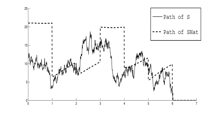
Figure 1: A simulated path of the full information value $h^{\text{stock}}(V_{t})$ of the stock (dashed line) and of the stock price ${S}$ (normal line, label SHat) for $c_{1}=c_{2}=0$ (only dividend information).

Next we show that more realistic asset price dynamics can be obtained by adding the filtration $\mathbb{F}^{Z}$ to the modelling filtration. In Figure 2 we plot a typical stock price trajectory together with the full information value $h^{\text{stock}}(V_{t})$ for the parameter values $c_{1}=4$ and $c_{2}=0$. Clearly, $S_{t}$ has nonzero volatility between dividend dates. A comparison of the two trajectories moreover shows that the stock price jumps to zero at the default time $\tau$; this reflects the fact that the default time has an intensity under incomplete information so that default comes as a surprise. The corresponding filter density $\pi(t)$ is plotted in Ficure 3

For comparison purposes we finally consider the parameter set $c_{1}=4,c_{2}=25$. For these parameter values default is “almost predictable” and the model behaves similar to a structural model. This can be seen from Figure 4 where we plot the default intensity for both parameter sets. Note that for $c_{1}=4,c_{2}=25$, the default intensity is close to zero most of the time and very large immediately prior to default (in fact almost twice as large as in the case where $c_{2}=0$.).

In Figure 5 we finally present the result of a small calibration exercise, where $\pi(t)$ was calibrated to five-year CDS spreads of Lehman brothers using the methodology described in the previous section. The data range over the period September 2006 to September 2008 (Lehman filed for bankruptcy protection on September 15, 2008). Since under full information CDS spreads are homogeneous of degree zero in $V$ and $K$, we took the default threshold equal to $K=1$ so that the numbers on the $x$-axis can be viewed as ratio of asset over liabilities. It can be seen clearly that prior to default the mass of $\pi(t)$ is concentrated close to the default threshold.

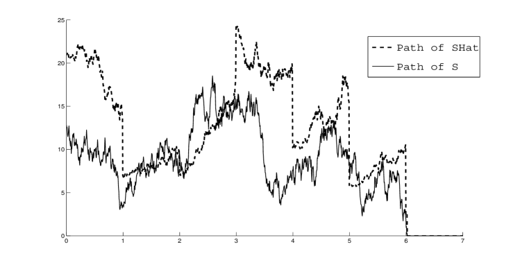
Figure 2: A simulated path of the full information value $h^{\text{stock}}(V_{t})$ of the stock (dashed line) and of the stock price ${S}_{t}$ (normal line, label Shat) for $c_{1}=4,c_{2}=0$.

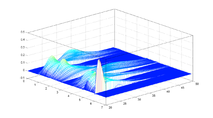
Figure 3: A simulated realisation of the conditional density $\pi(t)$. Note how the mass of $\pi(t)$ concentrates at the default threshold shortly before $\tau$.

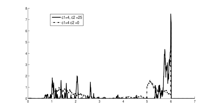
Figure 4: A simulated path of the default intensity for for $c_{1}=4,c_{2}=0$ (dashed) and for $c_{1}=4,c_{2}=25$ (straight line).

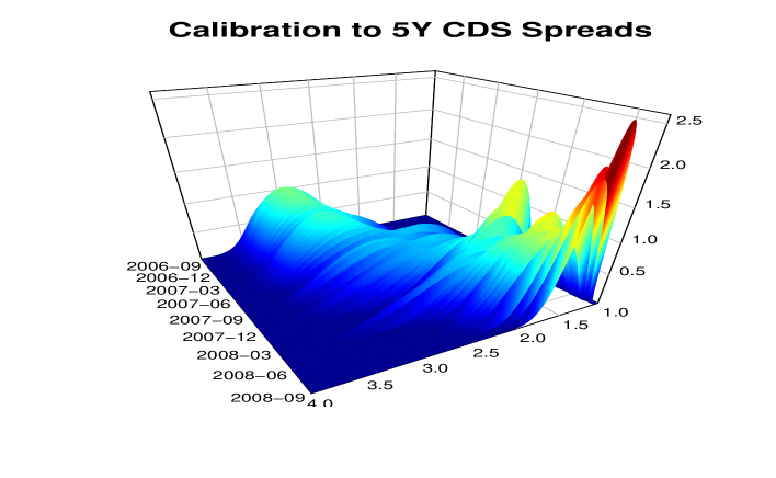
Figure 5: Result of a calibration of the filter density to 5-year CDS-spreads of Lehman brothers prior to default of the bank. In this example the default threshold is $K=1$.

8 Outlook and Conclusion

This paper has developed a theory of derivative asset analysis for structural credit risk models under incomplete information using stochastic filtering techniques. In particular we managed to derive the dynamics of traded securities which enabled us to study the pricing and the hedging of derivatives. To conclude we briefly mention a couple of financial problems where this theory could prove useful.

To begin with it might be interesting to study contingent convertible bonds, also known as CoCos, in our setup. A CoCo is a convertible bond that is automatically triggered once the issuing company (typically a financial institution) enters into financial distress. At the trigger event the bond is either converted into equity or into an immediate cash-payment that is substantially lower than the nominal value of the bond. Modelling the trigger mechanism adequately is a crucial part in the analysis of CoCos. The CoCos that have been issued so far have a so-called accounting trigger based on capital adequacy ratios. It is difficult to include this directly into a formal pricing model; many pricing approaches therefore model the conversion time $\tau^{\text{CoCo}}$ as a first passage time of the form $\tau^{\text{CoCo}}=\inf\{t\in\mathcal{T}\colon V_{t}\leq K^{\text{CoCo}}\}$ for a conversion threshold $K^{\text{CoCo}}>K$ and a set of monitoring dates $\mathcal{T}\subset[0,\infty)$. This valuation approach is however difficult to apply in practice, since investors are not able to track the asset value continuously in time, see for instance bib:spiegeleer-schoutens-12. Our setup is where $V$ is not fully observable is well-suited for dealing with this issue in a consistent manner. First results in this direction can be found in Chapter 5 of bib:roesler-16.

Our framework could also be used to study derivative asset analysis for sovereign bonds. Several fairly recent papers have proposed structural models with endogenous default for sovereign credit risk, see for instance bib:andrade-09 or bib:mayer-13. Roughly speaking, in these models default is given by a first passage time,

$$\tau=\inf\{t\geq 0\colon\tilde{V}_{t}\geq\tilde{K}_{t}\}=\inf\{t\geq 0\colon V_{t}:=\tilde{V}_{t}/\tilde{K}_{t}\leq 1\},$$

where the process $\tilde{V}$ is a measure of the expected future economic performance of the sovereign and where the threshold process $\tilde{K}$ is chosen by the sovereign in an attempt to balance the benefits accruing from lower debt services against the adverse economic implications of a default such as reduced access to capital markets. It is reasonable to assume that $\tilde{V}$ and $\tilde{K}$ are not fully observable for outside investors, for instance because it is hard to predict the outcome of the sovereign’s decision process in detail. Hence one is led to a model of the form (2.1) with “asset value $V=\tilde{V}/\tilde{K}$ and default threshold $K=1$. The results of the present paper can be used to derive the dynamics of sovereign credit spreads in this setup; this is important for the pricing of options on sovereign bonds and for risk management purposes.

Appendix A Additional Results

A.1 Filter equations.

In the next corollary we state the filtering equations for $\mathbb{F}^{\mathcal{M}}$.

Corollary A.1.

For $f\in C^{1,2}([0,T]\times S^{X})$ the optional projection $\widehat{f}_{t}$ has dynamics

$$\begin{split}\widehat{f}_{t}&=\widehat{f}_{0}+\int_{0}^{t}\Big{(}\widehat{\frac{df}{dt}}\Big{)}_{s}+(1-Y_{s-})(\widehat{\mathcal{L}_{X}f})_{s}\,ds+\int_{0}^{t\wedge\tau}(\widehat{fa})_{s}^{\top}-\widehat{f}_{s}\widehat{a}_{s}^{\top}\,dM_{s}^{Z,\mathbb{F}^{\mathcal{M}}}\\ &+\int_{0}^{t\wedge\tau}(f(s,K)-\widehat{f}_{s-})\,dM_{s}^{Y}+\int_{0}^{t\wedge\tau}\int_{\mathbb{R}^{+}}\Big{(}\frac{(\widehat{f(\cdot-\kappa y)\varphi(y,\cdot)})_{s-}}{(\widehat{\varphi(y)})_{s-}}-\widehat{f}_{s-}\Big{)}\;\mu^{D}(dy,ds)\,.\end{split}$$ (A.1)

Proof.

Recall that $\widehat{f}_{t}=1_{\{\tau\leq t\}}f(t,K)+1_{\{\tau>t\}}\pi_{t}f.$ Hence it holds that

$$d\widehat{f}_{t}=Y_{t-}\frac{df}{dt}(t,K)dt+\left(f(t,K)-\pi_{t}f\right)dY_{t}+(1-Y_{t-})d\pi_{t}f$$

Substituting the dynamics of $\pi_{t}f$ in this equation gives (A.1). ∎

Alternatively, one can derive the filter equations using the innovations approach to nonlinear filtering. For this one has to show first that every $\mathbb{F}^{\mathcal{M}}$ martingale can be represented as a sum of stochastic integrals with respect to the processes $Y_{t}-\Lambda_{t\wedge\tau}$ and $M^{Z,\mathbb{F}^{\mathcal{M}}}_{t}$, and with respect to the random measure measure $\mu^{D}-\gamma^{D,\mathbb{F}^{\mathcal{M}}}$. Standard arguments can then be used to identify the integrands in the martingale representation of $\widehat{f}_{t}-\int_{0}^{t}(\widehat{\mathcal{L}_{X}f})_{s}ds$. This is the route taken in bib:cetin-12 for the case without dividend payments.

A.2 Dynamic hedging

Next we give a few additional results related to our analysis of dynamic hedging in Section 6.2.

Computation of hedging strategies.

We now explain how the Itô formula for SPDEs can be used to compute the integrands in the martingale representation of an option on traded assets; this is needed during the application of Proposition 6.2.

We know from Section 6.1 that $\widetilde{\Pi}_{t}^{H}=\widetilde{C}^{H}(t,\pi(t))$ Using similar arguments as in the proof of Proposition 5.3, the dynamics of the conditional density $\pi(t)$ can be derived from the dynamics of $u(t)$ given in (4.25): for $t<\tau$ it holds that

$$\begin{split}d\pi(t)&=\big{(}\mathcal{A}^{*}\pi(t)+\pi(t)\lambda_{t}\big{)}dt+\pi(t)\big{(}a^{\top}-\widehat{a}^{\top}_{t}\big{)}dM_{t}^{Z}+\int_{\mathbb{R}^{+}}\!\!\frac{S_{\kappa y}\big{(}\pi(t-)\varphi(y,\cdot)\big{)}}{(\widehat{\varphi(y)})_{t-}}-\pi(t-)\,\mu^{D}(dy,dt)\,.\end{split}$$

Denote for $v\in H^{1}_{0}(S^{X})$ by $\widetilde{C}^{H}_{[v]}(t,\pi)$ the directional derivative of ${\widetilde{C}}^{H}$ in direction $v$, that is

$$\widetilde{C}^{H}_{[v]}(t,\pi)=\frac{d}{ds}{\Big{|}}_{s=0}\widetilde{C}^{H}(t,\pi+sv)\,.$$

Suppose that $\widetilde{C}^{H}$ satisfies the regularity conditions of bib:krylov-13 (essentially this means that the first and second directional derivative of $\widetilde{C}^{H}$ exists in every point $\pi\in H^{1}_{0}(S^{X})$). Then Theorem 3.1 of bib:krylov-13) gives the following martingale representation for the discounted option price:

$$\widetilde{C}^{H}(t,\pi(t)) =\widetilde{C}^{H}(0,\pi(0))+\sum_{i=1}^{l}\int_{0}^{t\wedge\tau}\!\!\widetilde{C}^{H}_{[\pi(s)(a^{i}-(\widehat{a^{i}})_{s})]}(s,\pi(s))\,dM_{s,i}^{Z}-\int_{0}^{t\wedge\tau}\!\!\widetilde{C}^{H}(s,\pi(s))\,dM^{Y}_{s}$$

$$+ \int_{0}^{t\wedge\tau}\!\!\int_{\mathbb{R}^{+}}\widetilde{C}^{H}\Big{(}s,\frac{S_{\kappa y}\big{(}\pi(s-)\varphi(y,\cdot)\big{)}}{(\widehat{\varphi(y)})_{s-}}\Big{)}-\widetilde{C}^{H}\big{(}s,\pi(s-)\big{)}\,(\mu^{D}-\gamma^{D,\mathbb{F}^{\mathcal{M}}})(dy,ds)\,.$$ (A.2)

In (A.2) the Itô formula for SPDEs is used to determine the integrands with respect to $dM_{s,i}^{Z}$; the integrands with respect to $M^{Y}$ and with respect to $(\mu^{D}-\gamma^{D,\mathbb{F}^{\mathcal{M}}})(dy,dt)$ can be determined by elementary arguments. All integrands (and hence the risk-minimizing hedging strategy) are functions of the current filter density $\pi(t)$; the practical computation of the directional derivative of $\widetilde{C}^{H}$ in the integral with respect to $M^{Z}$ (and of the other integrands) can be done with Monte Carlo. Note that we have not established the regularity of $\widetilde{C}$ required in bib:krylov-13; this very technical issue is left for future research.

Example A.2.

As a toy example we consider the problem of hedging an option with payoff $H=g(S_{T})$ using the stock as hedging instrument. To simplify the notation we consider the case where $Z$ is a one-dimensional process. First, we get from Proposition 6.2 that

$$\theta^{H}_{t}=\frac{\nicefrac{{d\langle\Pi^{H},\widetilde{G}^{\text{stock}}\rangle}}{{db}}\,(t)}{\nicefrac{{d\langle\widetilde{G}^{\text{stock}}\rangle}}{{db}}\,(t)}\,.$$

Between dividend dates, that is for $t\in[0,T]\setminus\mathcal{T}^{D}$ this gives

$$\theta^{H}_{t}=\frac{\big{(}({\widehat{h^{\text{stock}}}a})_{t}-\widetilde{S}_{t}\widehat{a}_{t}\big{)}\widetilde{C}^{H}_{[\pi(t)(a-\widehat{a}_{t})]}(t,\pi(t))+\lambda_{t}\widetilde{S}_{t-}\widetilde{C}^{H}(t,\pi(t-)}{\big{(}({\widehat{h^{\text{stock}}}a})_{t}-\widetilde{S}_{t-}\widehat{a}_{t-}\big{)}^{2}+\lambda_{t}^{2}\widetilde{S}_{t-}^{2}}\,;$$

at the dividend date $t_{n}$ we get

$$\theta^{H}_{t}=\frac{\displaystyle{\int_{\mathbb{R}^{+}}}\Big{(}\widetilde{C}\Big{(}t,\frac{S_{\kappa y}\big{(}\pi(t-)\varphi(y,\cdot)\big{)}}{(\widehat{\varphi(y)})_{t-}}\Big{)}-\widetilde{C}\big{(}t,\pi(t-))\Big{)}\Big{(}y+\frac{(\widehat{h^{\text{stock}}\varphi(y)})_{t-}}{(\widehat{\varphi(y)})_{t-}}-S_{t-}\Big{)}\,(\widehat{\varphi}(y))_{t-}dy}{\displaystyle{\int_{\mathbb{R}^{+}}}\Big{(}y+\frac{(\widehat{h^{\text{stock}}\varphi(y)})_{t-}}{(\widehat{\varphi(y)})_{t-}}-S_{t-}\Big{)}^{2}\,(\widehat{\varphi(y)})_{t-}dy}\,.$$

Market completeness.

Finally we discuss market completeness in our setup. For this we consider a variant of the model without dividend payments. This assumption is essential; with dividends the market is generically incomplete. Consider an option on traded assets with maturity $T$ and payoff $H$. Then the discounted price process $\widetilde{\Pi}^{H}$ has a martingale representation of the form

$$\widetilde{\Pi}^{H}_{t}=\widetilde{\Pi}^{H}_{0}+\sum_{j=1}^{l}\int_{0}^{t\wedge\tau}\xi_{s}^{M_{j}^{Z},H}dM_{s,j}^{Z}+\int_{0}^{t\wedge\tau}\xi_{s}^{Y,H}dM_{s}^{Y}\,.$$ (A.3)

As shown in Theorem 5.4, a similar representation holds for the discounted gains processes of the traded assets; the integrands are denoted by $\xi_{i}^{M_{j}^{Z}}$ and $\xi_{i}^{Y}$, $1\leq i\leq\ell,1\leq j\leq l$. A perfect hedging strategy $\theta^{*}$ satisfies for all $t\leq T$ the relation $\widetilde{\Pi}^{H}_{t}=\widetilde{\Pi}^{H}_{0}+\sum_{i=1}^{\ell}\int_{0}^{t}\theta^{*}_{s,i}d\widetilde{G}_{s,i}$; the cash position is determined from the selffinancing condition. Now we get that

$$\sum_{i=1}^{\ell}\int_{0}^{t}\theta^{*}_{s,i}d\widetilde{G}_{s,i}=\int_{0}^{t\wedge\tau}\sum_{j=1}^{l}\Big{(}\sum_{i=1}^{\ell}\theta^{*}_{s,i}\xi_{s,i}^{M_{j}^{Z}}\big{)}dM_{s,j}^{Z}+\int_{0}^{t\wedge\tau}\sum_{i=1}^{\ell}\theta^{*}_{s,i}\xi_{s,i}^{Y}dM_{s}^{Y}\,.$$ (A.4)

Comparing (A.3) and (A.4) we see that for $t\leq\tau$ a perfect replication strategy $\theta^{*}_{t}$ has to solve the following $l+1$ dimensional system of linear equations

$$\sum_{i=1}^{\ell}\theta^{*}_{t,i}\xi_{t,i}^{M_{j}^{Z}}=\xi_{t}^{M_{j}^{Z},H},\;1\leq j\leq j\,,\,\text{ and }\sum_{i=\ell}^{l}\theta^{*}_{t,i}\xi_{t,i}^{M^{Y}}=\xi_{t}^{M^{Y},H}.$$ (A.5)

Modulo integrability conditions, for every option on traded assets a perfect hedging therefore exists if and only if the system (A.5) has a solution for all $t\leq\tau$ and every right hand side $(\xi_{t}^{M_{1}^{Z},H},\dots,\xi_{t}^{M_{l}^{Z},H},\xi_{t}^{M^{Y},H})^{\top}$. Loosely speaking, for complete markets one thus needs to have for every $t<\tau$ at least $l+1$ locally independent traded assets. With dividend payments we would get an additional equation for every $y$ in the support of $\gamma^{D,\mathbb{F}^{\mathcal{M}}}(dy,\{t_{n}\})$ so that at $t_{n}$ (A.5) becomes a system with infinitely many equations for finitely many unknowns and hence generically unsolvable.

Appendix B Proofs

Proof of Lemma 3.2.

Define the gains process $G_{t}=V_{t}+D_{t}$, the discounted gains process

$$\widetilde{G}_{t}=e^{-rt}V_{t}+\int_{0}^{t}e^{-rs}dD_{s}=:\widetilde{V}_{t}+\widetilde{D}_{t}$$ (B.1)

and the cum-dividend asset value process $\bar{V}_{t}$ with $\bar{V}_{t}=V_{0}+\int_{0}^{t}r\bar{V}_{s}ds+\int_{0}^{t}\sigma\bar{V}_{s}dB_{s}$. We first show that $\widetilde{G}$ is a martingale. In fact, by (2.4) we have

$$d\widetilde{G}_{t}=\sigma\widetilde{V}_{t}dB_{t}-e^{-rt}dD_{t}+e^{-rt}dD_{t}=\sigma\widetilde{V}_{t}dB_{t}\,;$$

so that $\widetilde{G}$ is a local martingale. Moreover, $E^{Q}(\widetilde{V}_{t}^{2})\leq E^{Q}\big{(}(e^{-rt}\bar{V}_{t})^{2}\big{)}=e^{\sigma^{2}t}E^{Q}(V_{0}^{2})$. Hence we get

$$E^{Q}([\widetilde{G}]_{T})=E^{Q}\Big{(}\int_{0}^{T}\sigma^{2}\widetilde{V_{s}}^{2}ds\Big{)}\leq E^{Q}\Big{(}\int_{0}^{T}\sigma^{2}\big{(}e^{-rs}\bar{V}_{s}\big{)}^{2}ds\Big{)}<\infty\,,$$

and $\widetilde{G}$ is a square integrable true martingale. Now it obviously holds that $\sum_{t_{n}\geq 0}e^{-rt_{n}}d_{n}=\lim_{n\to\infty}\widetilde{D}_{t_{n}}$. Moreover, as $\widetilde{G}_{t_{n}}=\widetilde{V}_{t_{n}}+\widetilde{D}_{t_{n}}>\widetilde{D}_{t_{n}}$, one has $E^{Q}(\widetilde{D}_{t_{n}}\mid V_{0})\leq E^{Q}(\widetilde{G}_{t_{n}}\mid V_{0})=V_{0}$. Since $\widetilde{D}_{t_{n}}$ is an increasing process we get from monotone integration that

$$E^{Q}\Big{(}\sum_{t_{n}\geq 0}e^{-rt_{n}}d_{n}\mid V_{0}\Big{)}=E^{Q}\Big{(}\lim_{n\to\infty}\widetilde{D}_{t_{n}}\mid V_{0}\Big{)}=\lim_{n\to\infty}E^{Q}\big{(}\widetilde{D}_{t_{n}}\mid V_{0}\big{)}\leq V_{0}\,.$$ (B.2)

In order to show that one has equality in (B.2) we have to show that $\lim_{n\to\infty}E^{Q}\big{(}\widetilde{V}_{t_{n}}\mid V_{0}\big{)}=0$. We have the estimate

$$E^{Q}\Big{(}\sum_{t_{n}\geq 0}e^{-rt_{n}}d_{n}\mid V_{0}\Big{)}\geq E^{Q}\Big{(}\sum_{t_{n}\geq 0}\delta_{n}\widetilde{V}_{t_{n}}-\delta^{n}e^{-rt_{n}}K\mid V_{0}\Big{)}=E^{Q}(\delta_{1})\Big{(}\sum_{n\geq 0}E^{Q}\big{(}\widetilde{V}_{t_{n}}\mid V_{0}\big{)}-K\sum_{n\geq 0}e^{-rt_{n}}\Big{)}.$$ (B.3)

Recall that the dividend dates are equidistant by Assumption 2.1.2, so that $\sum_{n\geq 0}e^{-rt_{n}}<\infty$. Suppose now that there is some $c>0$ such that $E^{Q}\big{(}\widetilde{V}_{t_{n}}\mid V_{0}\big{)}>c$ for infinitely many $n$. Together with (B.3) this implies that $E^{Q}\Big{(}\sum_{t_{n}\geq 0}e^{-rt_{n}}d_{n}\mid V_{0}\Big{)}=\infty$, contradicting the inequality (B.2), and we conclude that $\lim_{n\to\infty}E^{Q}\big{(}\widetilde{V}_{t_{n}}\mid V_{0}\big{)}=0$. ∎

Proof of Identity (4.3).

This identity will follow from the relation

$$E^{Q}\big{(}h(V_{t})1_{\{\tau>t\}}\mid\mathcal{F}_{t}^{\mathcal{M}}\big{)}=E^{Q}\big{(}h(V_{t}^{\tau})1_{\{\tau>t\}}\mid\mathcal{F}_{t}^{Z^{\tau}}\vee\mathcal{F}_{t}^{Y}\big{)},$$ (B.4)

where $\mathbb{F}^{Z^{\tau}}$ is the filtration generated by the stopped process $Z^{\tau}$. To this, note first that $\mathbb{F}^{Z^{\tau}}\vee\mathbb{F}^{Y}$ is a subfiltration of $\mathbb{F}^{\mathcal{M}}$ (as $\tau$ is an $\mathbb{F}^{\mathcal{M}}$ stopping time), so that the right hand side of (B.4) is $\mathcal{F}_{t}^{\mathcal{M}}$-measurable. Moreover, for $\tau>t$ one has $V_{t}^{\tau}=V_{t}$ and $(Z_{s}^{\tau})_{s=0}^{t}=(Z_{s})_{s=0}^{t}$. Hence we get for any bounded measurable functional $g$ on $\mathcal{C}^{0}\big{(}[0,T])$ that

$$E^{Q}\big{(}h(V_{t})1_{\{\tau>t\}}g((Z_{s})_{s=0}^{t})\big{)} =E^{Q}\big{(}h(V_{t}^{\tau})1_{\{\tau>t\}}g((Z_{s}^{\tau})_{s=0}^{t})\big{)}$$

$$=E^{Q}\Big{(}E^{Q}\big{(}h(V_{t}^{\tau})1_{\{\tau>t\}}\mid\mathcal{F}_{t}^{Z^{\tau}}\vee\mathcal{F}_{t}^{Y}\big{)}g((Z_{s}^{\tau})_{s=0}^{t})\Big{)}\,.$$ (B.5)

Due to the presence of the indicator $1_{\{\tau>t\}}$ in (B.5) we may replace $g((Z_{s}^{\tau})_{s=0}^{t})$ with $g((Z_{s})_{s=0}^{t})$ in that equation, so that we obtain (B.4) by the definition of conditional expectations. A similar argument shows that $E^{Q}\big{(}h(V_{t})1_{\{\tau>t\}}\mid\mathcal{F}_{t}^{\tilde{Z}}\vee\mathcal{F}_{t}^{Y}\big{)}=E^{Q}\big{(}h(V_{t})1_{\{\tau>t\}}\mid\mathcal{F}_{t}^{Z^{\tau}}\vee\mathcal{F}_{t}^{Y}\big{)}$, which gives the equality

$$E^{Q}\big{(}h(V_{t})1_{\{\tau>t\}}\mid\mathcal{F}_{t}^{\mathcal{M}}\big{)}=E^{Q}\big{(}h(V_{t}^{\tau})1_{\{\tau>t\}}\mid\mathcal{F}_{t}^{\tilde{Z}}\vee\mathcal{F}_{t}^{Y}\big{)}\,,$$

as claimed. ∎

Proof of Proposition 4.2.

The process $F_{t}^{\sigma_{N}}=Q(\sigma_{N}\leq t\mid\mathcal{F}_{t})$, ${0\leq t\leq T}$, is an $\mathbb{F}$-submartingale. Hence we get, using the first submartingale inequality (see for instance bib:karatzas-shreve-88, Theorem 1.3.8(i))

$$Q\big{(}\sup_{s\leq T}F_{s}^{\sigma_{N}}>\epsilon\big{)}\leq\frac{1}{\epsilon}E\left((F_{T}^{\sigma_{N}})^{+}\right)=\frac{1}{\epsilon}Q(\sigma_{N}\leq T),$$

which gives Statement 1.

Now we turn to Statement 2. For the purposes of the proof we make the dependence of the stopped asset value process on $N$ explicit and we write $X_{t}^{N}:=V_{t}^{\tau\wedge\sigma^{N}}$. Clearly, on $\{\sigma_{N}>T\}$ it holds that $1_{\{\tau^{N}>t\}}=1_{\{\tau>t\}}$, $t\leq T$. Using Proposition 4.1 we thus get

$$Q\Big{(}\sup_{t\leq T}\Big{|}{1_{\{\tau^{N}>t\}}E^{Q}\big{(}h(t,V_{t}^{N})\mid\mathcal{F}_{t}^{\mathcal{M},N}\big{)}-1_{\{\tau>t\}}E^{Q}\big{(}h(t,V_{t})\mid\mathcal{F}_{t}^{\mathcal{M}}\big{)}}\Big{|}>\delta\Big{)}$$

$$\;\leq Q\bigg{(}\sup_{t\leq T}\Big{|}\frac{E^{Q}\big{(}h(t,X_{t}^{N})1_{\{X_{t}^{N}>K\}}\mid\mathcal{F}_{t}^{Z^{N}}\vee\mathcal{F}_{t}^{D^{N}}\big{)}}{Q\big{(}X_{t}^{N}>K\mid\mathcal{F}_{t}^{Z^{N}}\vee\mathcal{F}_{t}^{D^{N}}\big{)}}-\frac{E^{Q}\big{(}h(t,X_{t})1_{\{X_{t}>K\}}\mid\mathcal{F}_{t}^{Z}\vee\mathcal{F}_{t}^{D}\big{)}}{Q\big{(}X_{t}>K\mid\mathcal{F}_{t}^{Z}\vee\mathcal{F}_{t}^{D}\big{)}}\Big{|}>\delta\bigg{)}$$ (B.6)

$$\;+Q\big{(}\sigma_{N}>T\big{)}$$

Now $Q\big{(}\sigma_{N}>T\big{)}$ converges to zero for $N\to\infty$ so that we concentrate on (B.6). The difficulty in estimating this probability is the fact that we have to compare conditional expectations with respect to different filtrations. Similarly as in robust filtering, we address this problem using the reference probability approach. To ease the notation we introduce the abbreviations $h_{t}^{N}=h(t,X_{t}^{N})1_{\{X_{t}^{N}>K\}}$ and $h_{t}=h(t,X_{t})1_{\{X_{t}>K\}}\,.$ Moreover, we set

$$L_{t}^{1,N} =\exp\Big{(}\int_{0}^{t}a(X_{s}^{N})^{\top}dZ_{s}-\frac{1}{2}\int_{0}^{t}\bigl{|}a((X_{s}^{N}))\bigr{|}^{2}\,ds\Big{)}\;\text{ and }L_{t}^{2,N}=\prod_{t_{n}\leq T}\frac{\varphi(d_{n},X_{t_{n}-}^{N})}{\varphi^{*}(d_{n})}\,,$$

and we let $L_{t}^{N}:=L_{t}^{1,N}L_{t}^{2,N}$. The density martingale $L_{t}=L_{t}^{1}L_{t}^{2}$ is defined in analogously, but with $V^{\tau}$ instead of $X^{N}$. In view of Proposition 4.1 and (4.22) we need to show that for $N\to\infty$,

$$\sup_{t\leq T}\Big{|}\frac{E^{Q_{1}}\big{(}h_{t}^{N}L_{t}^{N}(\cdot,\omega_{2})\big{)}}{E^{Q_{1}}\big{(}1_{\{X_{t}^{N}>K\}}L_{t}^{N}(\cdot,\omega_{2})\big{)}}-\frac{E^{Q_{1}}\big{(}h_{t}L_{t}(\cdot,\omega_{2})\big{)}}{E^{Q_{1}}\big{(}1_{\{V_{t}^{\tau}>K\}}L_{t}(\cdot,\omega_{2})\big{)}}\Big{|}\overset{Q}{\longrightarrow}0\,.$$ (B.7)

The key tool for this is the following lemma.

Lemma B.1.

Consider a generic function $f\colon[0,T)\times[K,\infty)\to\mathbb{R}$ with $\bigl{|}f(t,v)\bigr{|}\leq c_{0}+c_{1}v$ and let $f_{t}^{N}=f(t,X_{t}^{N})$ and $f_{t}=f(t,V_{t}^{\tau}).$ Then it holds that

$$\sup_{t\leq T}\Big{|}E^{Q_{1}}\big{(}f_{t}^{N}L_{t}^{N}(\cdot,\omega_{2})\big{)}-E^{Q_{1}}\big{(}f_{t}L_{t}(\cdot,\omega_{2})\big{)}\Big{|}\overset{Q}{\longrightarrow}0.$$

Proof of Lemma B.1.

Fix constants $\epsilon,\delta>0$. We have to show that for $N$ sufficiently large,

$$Q_{2}\Big{(}\big{\{}\omega_{2}\colon\sup_{t\leq T}\Big{|}E^{Q_{1}}\big{(}f_{t}^{N}L_{t}^{N}(\cdot,\omega_{2})\big{)}-E^{Q_{1}}\big{(}f_{t}L_{t}(\cdot,\omega_{2})\big{)}\Big{|}>\delta\big{\}}\Big{)}<\epsilon$$ (B.8)

We first show that we may assume without loss of generality that $L_{t}^{2,N}$ and $L_{t}^{2}$ are bounded. To this we choose some constant $C$ such that $Q_{2}(B)>1-\frac{\epsilon}{2}$ where

$$B:=\Big{\{}\omega_{2}\colon\sup_{x\in[K,\infty)}\prod_{t_{n}\leq T}\frac{\varphi(d_{n}(\omega_{2}),x)}{\varphi^{*}(d_{n}(\omega_{2}))}\leq C\Big{\}}$$

This is possible since $\varphi^{*}$ is bounded away from zero on every compact subset of $(0,\infty)$ and since for fixed $d_{n}$ the mapping $x\mapsto\varphi(d_{n},x)$ is bounded by (2.5). By definition it holds on $B$ that $L_{t}^{2,N}=L_{t}^{2,N}\wedge C$ and $L_{t}^{2}=L_{t}^{2}\wedge C$. Moreover, (B.8) is no larger than

$$Q_{2}\bigg{(}\Big{\{}\sup_{t\leq T}\Big{|}E^{Q_{1}}\big{(}f_{t}^{N}L_{t}^{N,1}(L_{t}^{N,2}\wedge C)(\cdot,\omega_{2})\big{)}-E^{Q_{1}}\big{(}f_{t}L_{t}^{1}(L_{t}^{2}\wedge C)(\cdot,\omega_{2})\big{)}\Big{|}>\delta\Big{\}}\cap B\bigg{)}+Q(B^{c})$$

$$\quad\leq Q_{2}\Big{(}\sup_{t\leq T}\Big{|}E^{Q_{1}}\big{(}f_{t}^{N}L_{t}^{N,1}(L_{t}^{N,2}\wedge C)(\cdot,\omega_{2})\big{)}-E^{Q_{1}}\big{(}f_{t}L_{t}^{1}(L_{t}^{2}\wedge C)(\cdot,\omega_{2})\big{)}\Big{|}>\delta\Big{)}+\frac{\epsilon}{2}$$

Hence we assume from now on that $L_{t}^{2,N}$ and $L_{t}^{2}$ are bounded by $C$.

We continue with some useful estimates on $L_{t}$. Doob’s maximal inequality gives

$$E^{Q^{*}}\bigg{(}\sup_{0\leq t\leq T}(L_{t})^{2}\bigg{)} \leq C^{2}E^{Q^{*}}\Big{(}\sup_{0\leq t\leq T}(L_{t}^{1})^{2}\Big{)}\leq 4C^{2}E^{Q^{*}}\Big{(}(L_{T}^{1})^{2}\Big{)}=4C^{2}E^{Q^{*}}\bigg{(}\exp\Big{(}\int_{0}^{T}\left\|a(V_{s}^{\tau})\right\|^{2}ds\Big{)}\bigg{)}$$

$$\leq 4C^{2}\exp\Big{(}T\sup_{x\geq K}\left\|a(x)\right\|^{2}\Big{)}$$ (B.9)

Similarly we get for $\bar{V}_{t}=\tilde{V}_{0}\exp\big{(}(r-\frac{1}{2}\sigma^{2})t+\sigma B_{t}\big{)}$ (the cum-dividend asset value) that

$$E^{Q^{*}}\bigg{(}\sup_{0\leq t\leq T}(\bar{V}_{t}L_{t})^{2}\bigg{)} \leq C^{2}e^{2rT}E^{Q}(\tilde{V}_{0}^{2})E^{Q^{*}}\bigg{(}\sup_{0\leq t\leq T}\mathcal{E}\big{(}a(V_{s}^{\tau})^{\top}dZ_{s}+\sigma dB_{s}\big{)}_{t}\bigg{)}$$

$$\leq 4C^{2}e^{2rT}E^{Q^{*}}(\tilde{V}_{0}^{2})\exp\Big{(}T(\sigma^{2}+\sup_{x\geq K}\left\|a(x)\right\|^{2})\Big{)}$$ (B.10)

Of course, similar estimates hold for $E^{Q^{*}}\left(\sup_{0\leq t\leq T}(L_{t}^{N})^{2}\right)$ and for $E^{Q^{*}}\left(\sup_{0\leq t\leq T}(\bar{V}_{t}L_{t}^{N})^{2}\right)$. Since on the set $\{t<\sigma_{N}\}$, $f_{t}^{N}=f_{t}$ and $L_{t}^{N}=L_{t}$, it holds that

$$\Big{|}E^{Q_{1}}\big{(}f_{t}^{N}L_{t}^{N}(\cdot,\omega_{2})\big{)}-E^{Q_{1}}\big{(}f_{t}L_{t}(\cdot,\omega_{2})\big{)}\Big{|}\leq E^{Q_{1}}\Big{(}1_{\{\sigma_{N}\leq t\}}\bigl{|}f_{t}^{N}\bigr{|}L_{t}^{N}\big{(}\cdot,\omega_{2})\Big{)}+E^{Q_{1}}\Big{(}1_{\{\sigma_{N}\leq t\}}\bigl{|}f_{t}\bigr{|}L_{t}(\cdot,\omega_{2})\Big{)}.$$

Hence we get

$$\sup_{0\leq t\leq T}\Big{|}E^{Q_{1}}\big{(}f_{t}^{N}L_{t}^{N}(\cdot,\omega_{2})\big{)}-E^{Q_{1}}\big{(}f_{t}L_{t}(\cdot,\omega_{2})\big{)}\Big{|}$$

$$\quad\leq\sup_{0\leq t\leq T}E^{Q_{1}}\big{(}1_{\{\sigma_{N}\leq t\}}\bigl{|}f_{t}^{N}\bigr{|}L_{t}^{N}\big{(}\cdot,\omega_{2})\big{)}+\sup_{0\leq t\leq T}E^{Q_{1}}\big{(}1_{\{\sigma_{N}\leq t\}}\bigl{|}f_{t}\bigr{|}L_{t}(\cdot,\omega_{2})\big{)}.$$ (B.11)

Now note that by assumption $\bigl{|}f_{t}^{N}\bigr{|}\leq c_{0}+c_{1}X_{t}^{N}\leq c_{0}+c_{1}\bar{V}_{t}$. Hence (B.11) can be estimated by

$$\sup_{0\leq t\leq T}E^{Q_{1}}\Big{(}1_{\{\sigma_{N}\leq t\}}(c_{0}+c_{1}\bar{V}_{t})L_{t}^{N}(\cdot,\omega_{2})\Big{)}+\sup_{0\leq t\leq T}E^{Q_{1}}\Big{(}1_{\{\sigma_{N}\leq t\}}(c_{0}+c_{1}\bar{V}_{t})L_{t}(\cdot,\omega_{2})\Big{)}$$ (B.12)

In order to complete the proof of the lemma we finally show that the expression

$$E^{Q_{2}}\Big{(}\sup_{0\leq t\leq T}E^{Q_{1}}\big{(}1_{\{\sigma_{N}\leq t\}}(c_{0}+c_{1}\bar{V}_{t})L_{t}^{N}\big{(}\cdot,\omega_{2})\big{)}\Big{)}=E^{Q^{*}}\Big{(}\sup_{0\leq t\leq T}1_{\{\sigma_{N}\leq t\}}(c_{0}+c_{1}\bar{V}_{t})L_{t}^{N}\Big{)}$$

converges to zero for $N\to\infty$, that is $E^{Q_{1}}\big{(}1_{\{\sigma_{N}\leq t\}}(c_{0}+c_{1}\bar{V}_{t})L_{t}^{N}(\cdot,\omega_{2})\big{)}$ converges to zero in $L^{1}(\Omega_{2},\mathcal{F}_{2},Q_{2})$ and hence also in probability. Now note that our previous estimates (B.9) and (B.10) imply that the random variables $Y^{N}:=\sup_{0\leq t\leq T}1_{\{\sigma_{N}\leq t\}}(c_{0}+c_{1}\bar{V}_{t})$ are uniformly bounded in $L^{2}(\Omega,\mathcal{F},Q^{*})$ and hence uniformly integrable, so that the claim follows from the Lebesgue theorem. The same argument obviously applies to the second term in (B.12) which proves the Lemma. ∎

Finally we return to the proof of (B.7) and hence of Proposition 4.2. Fix constants $\epsilon,\delta>0$ and choose $M>0$ in such a way that for $A_{1},A_{2}$ with

$$A_{1}:=\big{\{}\omega_{2}\colon\inf_{t\leq T}E^{Q^{1}}\big{(}L_{t}(\cdot,\omega_{2})\big{)}>{2}/{M}\big{\}}\;\text{ and }A_{2}:=\big{\{}\omega_{2}\colon\sup_{t\leq T}E^{Q_{1}}\big{(}h_{t}L_{t}(\cdot,\omega_{2})\big{)}<M-\delta\big{\}}$$

it holds that $Q_{2}(A_{1}^{c})<\frac{\varepsilon}{4}$ and $Q_{2}(A_{2}^{c})<\frac{\varepsilon}{4}$. Choose finally $N_{0}$ large enough so that for $N>N_{0}$ it holds $Q_{2}(A_{3})>1-\frac{\varepsilon}{4}$ and $Q_{2}(A_{4})>1-\frac{\varepsilon}{4}$; here

$$A_{3} :=\big{\{}\omega_{2}\colon\sup_{t\leq T}\Big{|}E^{Q_{1}}\big{(}h_{t}^{N}L_{t}^{N}(\cdot,\omega_{2})\big{)}-E^{Q_{1}}\big{(}h_{t}L_{t}(\cdot,\omega_{2})\big{)}\big{|}<\frac{\delta}{2M}\big{\}}$$

$$A_{4} :=\big{\{}\omega_{2}\colon\sup_{t\leq T}\Big{|}E^{Q_{1}}\big{(}L_{t}^{N}1_{\{X_{t}^{N}>K\}}(\cdot,\omega_{2})\big{)}-E^{Q_{1}}\big{(}L_{t}1_{\{V_{t}^{\tau}>K\}}(\cdot,\omega_{2})\big{)}\big{|}<\frac{\delta}{2M}\big{\}}\,;$$

this is possible by Lemma B.1. Let $A=A_{1}\cap A_{2}\cap A_{3}\cap A_{4}$ and note that $Q(A)>1-\epsilon$. By definition of $A$ we have for $N>N_{0}$ and $\omega_{2}\in A$ the estimates $\sup_{t<T}E^{Q_{1}}\big{(}h_{t}^{N}L_{t}^{N}(\cdot,\omega_{2})\big{)}<{M}$ and $\inf_{t<T}E^{Q_{1}}\big{(}L_{t}^{N}(\cdot,\omega_{2})\big{)}>\frac{1}{M}$. Now the mean value theorem from standard calculus gives for $x,\tilde{x}$ and $y,\tilde{y}\in\mathbb{R}$ with $\bigl{|}x\bigr{|},\bigl{|}\tilde{x}\bigr{|}<M$ and $\bigl{|}y\bigr{|},\bigl{|}\tilde{y}\bigr{|}>\frac{1}{M}$ the estimate $\big{|}\frac{\tilde{x}}{\tilde{y}}-\frac{x}{y}\big{|}\leq M\left(\bigl{|}\tilde{x}-x\bigr{|}+\bigl{|}\tilde{y}-y\bigr{|}\right).$ Applying this estimate we get for $\omega_{2}\in A$ that

$$\sup_{t\leq T}\Big{|}\frac{E^{Q_{1}}\big{(}h_{t}^{N}L_{t}^{N}(\cdot,\omega_{2})\big{)}}{E^{Q_{1}}\big{(}1_{\{X_{t}^{N}>K\}}L_{t}^{N}(\cdot,\omega_{2})\big{)}}-\frac{E^{Q_{1}}\big{(}h_{t}L_{t}(\cdot,\omega_{2})\big{)}}{E^{Q_{1}}\big{(}1_{\{V_{t}^{\tau}>K\}}L_{t}(\cdot,\omega_{2})\big{)}}\Big{|}\leq M\sup_{t\leq T}\Big{\{}$$

$$\qquad\bigl{|}E^{Q_{1}}\big{(}h_{t}^{N}L_{t}^{N}(\cdot,\omega_{2})\big{)}-E^{Q_{1}}\big{(}h_{t}L_{t}(\cdot,\omega_{2})\big{)}\bigr{|}+\bigl{|}E^{Q_{1}}\big{(}L_{t}^{N}(\cdot,\omega_{2})1_{\{X_{t}^{N}>K\}}\big{)}-E^{Q_{1}}\big{(}L_{t}1_{\{V_{t}^{\tau}>K\}}(\cdot,\omega_{2})\big{)}\bigr{|}\Big{\}}$$

$$\quad\leq M\Big{(}\frac{\delta}{2M}+\frac{\delta}{2M}\Big{)}=\delta$$

∎

Proof of Lemma 4.6.

In order to show that $E^{Q^{*}}(L_{T})=1$ we use induction over the dividend dates $t_{n}$. For $t<t_{1}$, $L_{t}=L_{t}^{1}$ and $E^{Q^{*}}\big{(}L_{t}^{1}\big{)}=1$ by the Novikov criterion (recall that $a$ is bounded by assumption). Suppose now that the claim holds for $t<t_{n}$. We get that

$$E^{Q^{*}}\big{(}L_{t_{n}}\big{)}=E^{Q^{*}}\Big{(}L_{t_{n}-}\,\frac{\varphi(d_{n},X_{t_{n}-})}{\varphi^{*}(d_{n})}\Big{)}=E^{Q^{*}}\Big{(}L_{t_{n}-}\,E^{Q^{*}}\Big{(}\frac{\varphi(d_{n},X_{t_{n}-})}{\varphi^{*}(d_{n})}\mid\mathcal{F}_{t_{n}-}\Big{)}\Big{)}.$$

Moreover,

$$E^{Q^{*}}\Big{(}\frac{\varphi(d_{n},X_{t_{n}-})}{\varphi^{*}(d_{n})}\mid\mathcal{F}_{t_{n}-}\Big{)}=\int_{\mathbb{R}^{+}}\frac{\varphi(y,X_{t_{n}-})}{\varphi^{*}(y)}\varphi^{*}(y)dy=\int_{\mathbb{R}^{+}}{\varphi(y,X_{t_{n}-})}\,dy=1\,,$$

so that $E^{Q^{*}}(L_{t_{n}}=1)$ as well.

In order to show that $\mu^{D}(dy,dt)$ has $Q$-compensator $\gamma^{D}(dy,dt)$ we use the general Girsanov theorem (see for instance bib:protter-05, Theorem 3.40): a process $M$ such that $\langle M,L\rangle$ exists for $Q^{*}$ is a $Q^{*}$-local martingale if and only if $\widetilde{M}_{t}=M_{t}-\int_{0}^{t}\frac{1}{L_{s}-}d\langle L,M\rangle_{s}$ is a $Q$-local martingale.

Consider now some bounded predictable function $\beta\colon[0.T]\times\mathbb{R}^{+}\to\mathbb{R}$ and define the $Q^{*}$-local martingale $M_{t}=\int_{0}^{t}\int_{\mathbb{R}^{+}}\beta(s,y)\,(\mu^{D}-\gamma^{D,*})(dy,ds)$. As $M$ is of finite variation, we get that

$$[M,L]_{t}=\sum_{s\leq t}\Delta M_{s}\Delta L_{s}=\int_{0}^{t}\int_{\mathbb{R}^{+}}L_{s-}\big{(}\frac{\varphi(y,X_{s-})}{\varphi^{*}(y)}-1\big{)}\beta(s,y)\mu^{D}(dy,ds).$$

Hence we get that

$$\langle M,L\rangle_{t} =\int_{0}^{t}\int_{\mathbb{R}^{+}}L_{s-}\big{(}\frac{\varphi(y,X_{s-})}{\varphi^{*}(y)}-1\big{)}\beta(s,y)\gamma^{D,*}(dy,ds)\,,$$ (B.13)

provided that

$$E^{Q^{*}}\Big{(}\int_{0}^{t}\int_{\mathbb{R}^{+}}L_{s-}\big{|}\frac{\varphi(y,X_{s-})}{\varphi^{*}(y)}-1\big{|}|\beta(s,y)|\gamma^{D,*}(ds,dy)\Big{)}<\infty\,.$$ (B.14)

Recall that $\gamma^{D,*}(dy,dt)=\sum_{n=1}^{\infty}\varphi^{*}(y)dy\,\delta_{\{t_{n}\}}(dt)$. Hence

$$\int_{0}^{t}\int_{\mathbb{R}^{+}}L_{s-}\big{|}\frac{\varphi(y,X_{s-})}{\varphi^{*}(y)}-1\big{|}\gamma^{D,*}(ds,dy)=\sum_{t_{n}\leq t}L_{t_{n}-}\int_{\mathbb{R}^{+}}\big{|}\varphi(y,X_{t_{n}-})-\varphi^{*}(y)\big{|}dy\leq 2\sum_{t_{n}\leq t}L_{t_{n}-}.$$

Since $|\beta|$ is bounded by some constant $C$ and since $E^{Q^{*}}(L_{t})=1$ for all $t$, the lhs of (B.14) is bounded by $2C\sup\{n\in\mathbb{N}\colon t_{n}\leq t\}$. Moreover, we get from (B.13) that

$$\langle M,L\rangle_{t}=\sum_{t_{n}\leq t}L_{t_{n}-}\int_{\mathbb{R}^{+}}\beta(t_{n},y)\big{(}\varphi(y,X_{t_{n}-})-\varphi^{*}(y)\big{)}dy$$

This gives

$$\widetilde{M}_{t}:=M_{t}-\int_{0}^{t}\frac{1}{L_{s}-}d\langle L,M\rangle_{s}=\int_{0}^{t}\int_{\mathbb{R}^{+}}\beta(s,y)(\mu^{D}-\gamma^{D})(dy,ds)\,.$$

Now $\widetilde{M}$ is a local martingale by the general Girsanov theorem, which shows that $\gamma^{D}(dy,dt)$ is in fact the $Q$-compensator of $\mu^{D}$. The other claims are clear. ∎

Proof of Theorem 4.7.

We proceed via induction over the dividend dates. For $t\in[0,t_{1})$ there is no dividend information and the claim follows from Theorem 4.4. Suppose now that the claim of the theorem holds for $t\in[0,t_{n})$. First we show that

$$u(t_{n})=S_{\kappa d_{n}}(\tilde{u}(t_{n}))=u(t_{n-},x+\kappa d_{n})\frac{\varphi(d_{n},x+\kappa d_{n})}{\varphi^{*}(d_{n})}$$

belongs to $H^{1}_{0}(S^{X})\cap H^{2}(S^{X})$. Clearly, under Assumption 2.12, for a given $d_{n}>0$, the mapping $x\mapsto{\varphi(d_{n},x)}\big{/}{\varphi^{*}(d_{n})}$ is smooth, nonnegative and bounded. Hence with $u(t_{n-})$ also $\tilde{u}(t_{n}))$ belongs to $H^{1}_{0}(S^{X})\cap H^{2}(S^{X})$. If $\kappa=1$ it remains to show that $S_{d_{n}}(\tilde{u}(t_{n}))$ is an element of $H^{1}_{0}(S^{X})\cap H^{2}(S^{X})$. Smoothness is clear, the only thing that needs to be verified is the boundary condition $\tilde{u}(t_{n},K+d_{n})=0\,.$ To this note that $\varphi(d_{n},z)=0$ for $z\leq d_{n}+K$ (see equation (2.3)). This implies that $\tilde{u}(t_{n},K+d_{n})=0$ as required. Existence and uniqueness of a solution of (4.25) on $[t_{n},t_{n+1})$ follows then immediately from Theorem 4.4.

Next we turn to the second claim. Using the induction hypothesis, the definition of $\tilde{u}$, the fact that $\varphi(d_{n},K)=\varphi^{*}(d_{n})$ and the dynamics of $\nu_{K}(t)$ and $\nu_{N}(t)$ we get that

$$\Sigma_{t_{n}}f =E^{Q^{*}}\Big{(}L_{t_{n}-}f(X_{t_{n}})\frac{\varphi(d_{n},X_{t_{n}-})}{\varphi^{*}(d_{n})}\Big{)}$$

$$=\big{(}u(t_{n}-),f(\cdot-\kappa d_{n})\frac{\varphi(d_{n},\cdot)}{\varphi^{*}(d_{n})}\big{)}_{S^{X}}+\nu_{K}(t_{n}-)f(K)\frac{\varphi(d_{n},K)}{\varphi^{*}(d_{n})}+\nu_{N}(t_{n}-)f(N)\frac{\varphi(d_{n},N)}{\varphi^{*}(d_{n})}$$

$$=\big{(}\tilde{u}(t_{n}-),f(\cdot-\kappa d_{n})\big{)}_{S^{X}}+\nu_{K}(t_{n})f(K)+\nu_{N}(t_{n})f(N).$$

Now we have

$$\big{(}\tilde{u}(t_{n}),f(\cdot-\kappa d_{n})\big{)}_{S^{X}} =\int_{K}^{N}f(x-\kappa d_{n})\tilde{u}(t_{n},x)dx=\int_{K-\kappa d_{n}}^{N-\kappa d_{n}}f(y)\tilde{u}(t_{n},y+\kappa d_{n})\,dy$$

$$=\int_{K}^{N}f(y)\tilde{u}(t_{n},y+\kappa d_{n})\,dy,$$

as the integrand is zero on $[K-\kappa d_{n},K]\cup[N-\kappa d_{n},N]$. Hence we get that

$$\big{(}\tilde{u}(t_{n}),f(\cdot-\kappa d_{n})\big{)}_{S^{X}}=\big{(}u(t_{n}),f\big{)}_{S^{X}}$$

and thus the relation $\Sigma_{t_{n}}f=\big{(}u(t_{n}),f\big{)}_{S^{X}}+\nu_{K}(t_{n})f(K)+\nu_{N}(t_{n})f(N)$ as claimed. ∎

Proof of Lemma 5.3.

We start with the case without dividends and we assume that $f$ is time-independent. Recall from Corollary 4.8 that $\pi_{t}f=\frac{1}{C(t)}\left((u(t),f)_{S^{X}}+\nu_{N}(t)f(N)\right)$ with $C(t)=(u(t),1)_{S^{X}}+\nu_{N}(t)$. Using (4.18) and (4.17) we get

$$dC(t)=\Big{(}\big{(}\mathcal{L}^{*}u(t),1\big{)}_{S^{X}}-\frac{1}{2}\sigma^{2}N^{2}\frac{du}{dx}(t,N)\Big{)}\,dt+\left(\big{(}u(t),a^{\top}\big{)}_{S^{X}}+\nu_{N}(t)a^{\top}(N)\right)dZ_{t}.$$ (B.15)

Partial integration shows that the drift term in (B.15) equals $-\frac{1}{2}\sigma^{2}K^{2}\frac{du}{dx}(t,K)$. Hence,

$$d\frac{1}{C(t)} =\frac{1}{2C(t)^{2}}\sigma^{2}K^{2}\frac{du}{dx}(t,K)\,dt-\frac{1}{C(t)^{2}}\left(\big{(}u(t),a^{\top}\big{)}_{S^{X}}+\nu_{N}(t)a^{\top}(N)\right)\,dZ_{t}$$

$$+\frac{1}{C(t)^{3}}\sum_{j=1}^{l}\big{(}\big{(}u(t),a_{j}\big{)}_{S^{X}}+\nu_{N}(t)a_{j}\big{)}^{2}\,dt\,.$$

Similarly, we obtain that

$$\begin{split}d\Big{(}\big{(}u(t),f\big{)}_{S^{X}}+\nu_{N}(t)f(N)\Big{)}&=\Big{(}\big{(}u(t),\mathcal{L}_{X}f\big{)}_{S^{X}}-\frac{1}{2}\sigma^{2}K^{2}\frac{du}{dx}(t,K)f(K)\Big{)}\,dt\\ &+\Big{(}\big{(}u(t),a^{\top}f\big{)}_{S^{X}}+\nu_{N}(t)a^{\top}(N)f(N)\Big{)}\,dZ_{t}.\end{split}$$ (B.16)

Hence we get, using the Itô product formula and the fact that $\pi(t,v)=u(t,v)/C(t)$

$$d\pi_{t}f= \frac{1}{C(t)}d\left(\big{(}u(t),f\big{)}_{S^{X}}+\nu_{N}(t)f(N)\right)+\left(\big{(}u(t),f\big{)}_{S^{X}}+\nu_{N}(t)f(N)\right)d\frac{1}{C(t)}$$

$$\hskip 89.626pt+d\,\big{[}\frac{1}{C},\big{(}u,f\big{)}_{S^{X}}+\nu_{N}f(N)\big{]}_{t}$$

$$= \Big{(}\big{(}\pi(t),\mathcal{L}_{X}f\big{)}_{S^{X}}-\frac{1}{2}\sigma^{2}K^{2}\frac{d\pi}{dx}(t,K)f(K)\Big{)}\,dt+\pi_{t}(a^{\top}f)\,dZ_{t}$$

$$+ \Big{(}\frac{1}{2}\sigma^{2}K^{2}\frac{d\pi}{dx}(t,K)\,\pi_{t}f+\sum_{j=1}^{l}(\pi_{t}a_{j})^{2}\pi_{t}f\Big{)}\,dt\ -(\pi_{t}f)(\pi_{t}a^{\top})\,dZ_{t}-\Big{(}\sum_{j=1}^{l}(\pi_{t}a_{j})(\pi_{t}a_{j}f)\Big{)}\,dt\,.$$

Rearranging terms and using that $\pi_{t}(\mathcal{L}_{X}f)=(\pi(t),\mathcal{L}_{X}f)_{S^{X}}$ gives the claim of the lemma for the case of time-independent $f$ and no dividends. For time-dependent $f$ we have $d\pi_{t}f=\pi_{t}(\frac{df}{dt}(t,\cdot))\,dt+d\pi_{t}f(t,\cdot)$ so that we obtain the additional term $\pi_{t}(\frac{df}{dt}(t,\cdot))$ in the drift of the dynamics of $\pi_{t}f$.

Finally, we consider the case with dividend payments. Between dividend dates the dynamics of $\widehat{f}_{t}$ can be derived by similar arguments as before. To derive the jump of $\pi_{t}f$ at $t_{n}$ recall that $\pi_{t_{n}}f=\Sigma_{t_{n}}(f1_{(K,\infty)})\big{/}\Sigma_{t_{n}}(1_{(K,\infty)})$. Moreover we have, using the form of $L_{t_{n}}$,

$$\Sigma_{t_{n}}(f1_{(K,\infty)})=\frac{1}{\varphi^{*}(d_{n})}\Sigma_{t_{n}-}\Big{(}f(\cdot-\kappa d_{n})1_{(K,\infty)}(\cdot-\kappa d_{n})\varphi(d_{n},\cdot)\Big{)}$$

and similarly for $\Sigma_{t_{n}}(1_{(K,\infty)})$. Now, by Assumption 2.12 we know that $d_{n}<(X_{t_{n}}-K)^{+}$ $Q$ a.s, so that $1_{(K,\infty)}(X_{t_{n}-}-\kappa d_{n})=1_{(K,\infty)}(X_{t_{n}-})$. Hence we get

$$\pi_{t_{n}}f =\frac{\Sigma_{t_{n}}(f1_{(K,\infty)})\big{/}\Sigma_{t_{n}-}(1_{(K,\infty)})}{\Sigma_{t_{n}}(1_{(K,\infty)})\big{/}\Sigma_{t_{n}-}(1_{(K,\infty)})}=\frac{\Sigma_{t_{n}-}\big{(}f(\cdot-\kappa d_{n})1_{(K,\infty)}\varphi(d_{n},\cdot)\big{)}\big{/}\Sigma_{t_{n}-}(1_{(K,\infty)})}{\Sigma_{t_{n}}\big{(}1_{(K,\infty)}\varphi(d_{n},\cdot)\big{)}\big{/}\Sigma_{t_{n}-}(1_{(K,\infty)})}$$

$$=\frac{\pi_{t_{n}-}\big{(}f(\cdot-\kappa d_{n})\varphi(d_{n},\cdot)\big{)}}{\pi_{t_{n}-}\big{(}\varphi(d_{n},\cdot)\big{)}},$$

which gives the form of the integral with respect to $\mu^{D}(dy,ds)$ in (A.1). ∎

References

- [1] \harvarditemAdams and Fournier2003bib:adams-fournier-03 Adams, R. and Fournier, J. F.: 2003, Sobolev Spaces, 2nd edn, Academic Press.
- [2] \harvarditemAndrade2009bib:andrade-09 Andrade, S. C.: 2009, A model of asset pricing under country risk, Journal of International Money and Finance 28, 671–696.
- [3] \harvarditemBain and Crisan2009bib:bain-crisan-08 Bain, A. and Crisan, D.: 2009, Fundamentals of Stochastic Filtering, Springer, New York.
- [4] \harvarditemBlack and Cox1976bib:black-cox-76 Black, F. and Cox, J. C.: 1976, Valuing corporate securities: Some effects of bond indenture provisions, The Journal of Finance 31(2), 351–367.
- [5] \harvarditemBlanchet-Scalliet and Jeanblanc2004bib:blanchet-scalliet-jeanblanc-04 Blanchet-Scalliet, C. and Jeanblanc, M.: 2004, Hazard rate for credit risk and hedging defaultable contingent claims, Finance and Stochastics 8, 145–159.
- [6] \harvarditemBrémaud1981bib:bremaud-81 Brémaud, P.: 1981, Point Processes and Queues: Martingale Dynamics, Springer, New York.
- [7] \harvarditemCetin2012bib:cetin-12 Cetin, U.: 2012, On absolutely continuous compensators and nonlinear filtering equations in default risk models, Stochastic Processes and their Applications 122, 3619–3647.
- [8] \harvarditem[Coculescu et al.]Coculescu, Geman and Jeanblanc2008bib:coculescu-geman-jeanblanc-06 Coculescu, D., Geman, H. and Jeanblanc, M.: 2008, Valuation of default sensitive claims under imperfect information, Finance and Stochastics 12, 195–218.
- [9] \harvarditem[Duffie et al.]Duffie, Eckner, Horel and Saita2009bib:duffie-et-al-06 Duffie, D., Eckner, A., Horel, G. and Saita, L.: 2009, Frailty correlated default, The Journal of Finance 64, 2089–2123.
- [10] \harvarditemDuffie and Lando2001bib:duffie-lando-01 Duffie, D. and Lando, D.: 2001, Term structure of credit risk with incomplete accounting observations, Econometrica 69, 633–664.
- [11] \harvarditem[Elliott et al.]Elliott, Jeanblanc and Yor2000bib:elliott-jeanblanc-yor-00 Elliott, R. J., Jeanblanc, M. and Yor, M.: 2000, On models of default risk, Mathematical Finance 10, 179–195.
- [12] \harvarditemFöllmer and Schweizer1989bib:foellmer-schweizer-89 Föllmer, H. and Schweizer, M.: 1989, hedging by sequential regression: An introduction to the mathematics of option trading, ASTIN Bulletin 18, 147–160.
- [13] \harvarditemFöllmer and Sondermann1986bib:foellmer-sondermann-86 Föllmer, H. and Sondermann, D.: 1986, Hedging of non-redundant contingent-claims, in W. Hildenbrand and A. Mas-Colell (eds), Contributions to Mathematical Economics, North Holland, pp. 147–160.
- [14] \harvarditemFrey and Runggaldier2010bib:frey-runggaldier-10 Frey, R. and Runggaldier, W.: 2010, Pricing credit derivatives under incomplete information: A nonlinear filtering approach, Finance and Stochastics 14, 495–526.
- [15] \harvarditemFrey and Schmidt2009bib:frey-schmidt-09b Frey, R. and Schmidt, T.: 2009, Pricing corporate securities under noisy asset information, Mathematical Finance 19, 403 – 421.
- [16] \harvarditemFrey and Schmidt2012bib:frey-schmidt-12 Frey, R. and Schmidt, T.: 2012, Pricing and hedging of credit derivatives via the innovations approach to nonlinear filtering, Finance and Stochastics 12, 105–133.
- [17] \harvarditem[Frey et al.]Frey, Schmidt and Xu2013bib:frey-schmidt-xu-13 Frey, R., Schmidt, T. and Xu, L.: 2013, On Galerkin approximations for the Zakai equation with diffusive and point process observations, SIAM Journal on Numerical Analysis 51, 2036–2062.
- [18] \harvarditemGermani and Piccioni1987bib:germani-piccioni-87 Germani, A. and Piccioni, M.: 1987, Finite-dimensional approximations for the equations of nonlinear filtering derived in mild form, Applied Mathematics and Optimization 16(1), 51–72.
- [19] \harvarditemHull and White2006bib:hull-white-06 Hull, J. C. and White, A.: 2006, The implied copula model, The Journal of Derivatives 14, 8–28.
- [20] \harvarditemJacod and Shiryaev2003bib:jacod-shiryaev-03 Jacod, J. and Shiryaev, A. S.: 2003, Limit Theorems for Stochastic Processes, 2nd edn, Springer, Berlin.
- [21] \harvarditemJarrow and Protter2004bib:jarrow-protter-04 Jarrow, R. A. and Protter, P.: 2004, Structural versus reduced-form models: a new information based perspective, Journal of Investment Management 2, 1–10.
- [22] \harvarditemJeanblanc and Shiriayev1995bib:jeanblanc-shiriayev-95 Jeanblanc, M. and Shiriayev, A.: 1995, Optimization of the flow of dividends, Russian Mathematical Surveys 50, 257–277.
- [23] \harvarditemKaratzas and Shreve1988bib:karatzas-shreve-88 Karatzas, I. and Shreve, S. E.: 1988, Brownian Motion and Stochastic Calculus, Springer, Berlin.
- [24] \harvarditemKrylov2013bib:krylov-13 Krylov, N.: 2013, A relatively short proof of Itô’s formula for SPDEs and its applications, Stochastic Partial Differential Equations: Analysis and Computation 1, 152–174.
- [25] \harvarditemKrylov and Wang2011bib:krylov-wang-11 Krylov, N. and Wang, T.: 2011, Filtering partially observable diffusions up to the first exit time from a domain, Stochastic Processes and their Applications 121, 1785–1815.
- [26] \harvarditemKusuoka1999bib:kusuoka-99 Kusuoka, S.: 1999, A remark on default risk models, Advances in Mathematical Economics 1, 69–81.
- [27] \harvarditemLando1998bib:Lando-98 Lando, D.: 1998, Cox processes and credit risky securities, Review of Derivatives Research 2, 99–120.
- [28] \harvarditemLe Gland1992bib:leGland-92 Le Gland, F.: 1992, Splitting-up approximation for SPDEs and SDEs with application to nonlinear filtering, Lecture Notes in Control and Information Sciences 176, 177–187.
- [29] \harvarditemLeland1994bib:leland-94 Leland, H. E.: 1994, Corporate debt value, bond covenants, and optimal capital structure, The Journal of Finance 49(4), 157–196.
- [30] \harvarditemLeland and Toft1996bib:leland-toft-96 Leland, H. E. and Toft, K.: 1996, Optimal capital structure, endogenous bankruptcy and the term structure of credit spreads, The Journal of Finance 51, 987–1019.
- [31] \harvarditemMayer2013bib:mayer-13 Mayer, M.: 2013, Sovereign credit risk and banking crises, Preprint, WU Vienna.
- [32] \harvarditemPardoux1978bib:pardoux-78 Pardoux, E.: 1978, Filtrage de diffusions avec condition frontières, Séminaire de Probabilités XII, Lecture Notes in Mathematics, Vol. 636, Springer, Berlin, pp. 163–188.
- [33] \harvarditemPeszat and Zabczyk2007bib:peszat-zabcyk-07 Peszat, P. and Zabczyk, J.: 2007, Stochastic Partial Differential Equations with Lévy Noise, Cambridge University Press.
- [34] \harvarditemProtter2005bib:protter-05 Protter, P.: 2005, Stochastic Integration and Differential Equations: A New Approach, second edn, Springer, Berlin.
- [35] \harvarditemRösler2016bib:roesler-16 Rösler, L.: 2016, Stochastic Filtering in Pricing and Credit Risk Management, PhD thesis, TU Wien. available from http://katalog.ub.tuwien.ac.at/AC13002123.
- [36] \harvarditemSchweizer2001bib:schweizer-01b Schweizer, M.: 2001, A guided tour through quadratic hedging approaches, in E. Jouini, J. Cvitanic and M. Musiela (eds), Option Pricing, Interest Rates and Risk Management, Cambridge University Press, Cambridge, pp. 538–574.
- [37] \harvarditemSpiegeleer and Schoutens2012bib:spiegeleer-schoutens-12 Spiegeleer, J. and Schoutens, W.: 2012, Pricing contingent convertibles: A derivatives approac, The Journal of Derivatives 20, 27–36.
- [38] \harvarditem[Sun et al.]Sun, Munves and Hamilton2012bib:moodys-edf-12 Sun, Z., Munves, D. and Hamilton, D.: 2012, Public Firm Expected Default Frequency Credit Measures: Methodology, Performance, and Model Extensions, Moody’s Analytics.
- [39] \harvarditemVellekoop and Nieuwenhuis2006bib:vellekoop-nieuwenhuis-06 Vellekoop, M. and Nieuwenhuis, J.: 2006, Efficient pricing of derivatives on assets with discrete dividends, Applied Mathematical Finance 13(6), 265–284.
- [40]