Facets on the convex hull of $d$-dimensional Brownian and Lévy motion

Abstract

For stationary, homogeneous Markov processes (viz., Lévy processes, including Brownian motion) in dimension $d\geq 3$, we establish an exact formula for the average number of $(d-1)$-dimensional facets that can be defined by $d$ points on the process’s path. This formula defines a universality class in that it is independent of the increments’ distribution, and it admits a closed form when $d=3$, a case which is of particular interest for applications in biophysics, chemistry and polymer science.

We also show that the asymptotical average number of facets behaves as $\langle\mathcal{F}_{T}^{(d)}\rangle\sim 2\left[\ln\left(T/\Delta t\right)\right]^{d-1}$, where $T$ is the total duration of the motion and $\Delta t$ is the minimum time lapse separating points that define a facet.

Introduction

Stochastic processes’ paths are common in the physical and natural sciences, in particular as models of actual motion Einstein (1905); Chandrasekhar (1949); Viswanathan et al. (2011); Bénichou et al. (2005), interfaces Havlin et al. (1991) or long proteins and other polymers Edwards (1965); De Gennes (1976); Westwater (1980); Doi and Edwards (1988). Spatial characteristics of stochastic processes thus come to reflect physically meaningful variables: home ranges of animals Worton (1987), heights of surfaces Majumdar and Comtet (2004), shapes of molecules Haber et al. (2000); Cook and Marenduzzo (2009).

One way to describe the spatial extent of a stochastic process’s path is to examine its convex hull. That is, the smallest convex set enclosing all points visited by the process. In two dimensions, exact expressions for the values of geometric quantities such as the mean perimeter or the mean area of the convex hull have been found for Brownian motion Takács (1980); El Bachir (1983); Biane and Letac (2011); Cranston et al. (1989) as well as for other types of stochastic motions Reymbaut et al. (2011); Kampf et al. (2012); Luković et al. (2013), for multi-walker systems Randon-Furling et al. (2009) and for confined configurations Chupeau et al. (2015a, b). In some cases, equivalent results exist in higher dimensional space Kinney (1966); Randon-Furling (2009); Davydov (2012); Kampf et al. (2012); Eldan (2014); Molchanov and Wespi (2016).

Results Rudnick and Gaspari (1987); Fougère and Desbois (1993); Haber et al. (2000) pertaining to the shape of such random convex hulls appear scarcer though, despite their importance in biophysics: a protein’s or an antibody’s ability to play its part depends crucially on its shape Alberts et al. (2002); Wilson et al. (2009). Convex hulls methods are central in the description of long-molecule configurations  Holm and Sander (1993); Meier et al. (1995); Lee et al. (2006); Stout et al. (2008); Wang et al. (2006), leading to questions on the structure of these hulls, such as on their number of edges (in 2D) or facets (in 3D) and on the distribution of distances between the molecule and its convex hull’s edges or facets Badel-Chagnon et al. (1994); Coleman and Sharp (2006).

Only recently, the average number of edges on the boundary of the convex hull of a vast class of planar random walks was computed. Remarkably, this was found to have a universal form: it grows logarithmically with time Randon-Furling (2014), whatever the distribution of the infinitesimal increments along the process’s path – as long as these increments are independent and identically distributed (i.e. as long as the process is what is called a Lévy process).

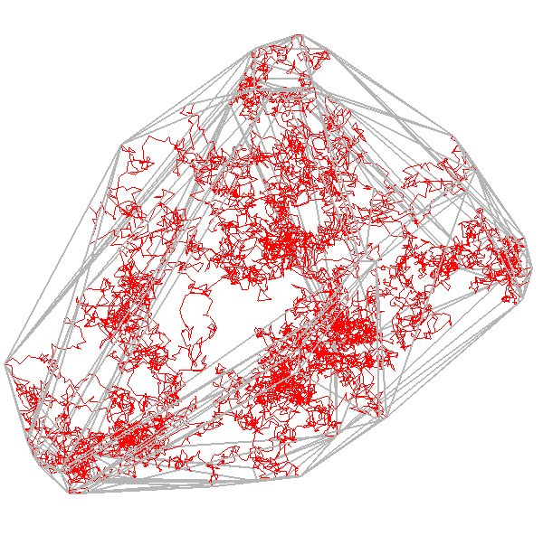
Figure 1: A sample realization of 3-dimensional Brownian motion and the facets on the boundary of its convex hull.

In this paper, we show that the universality observed for the average number of edges in two dimensions extends to the average number of facets in $d\geq 3$ dimensions (Fig.1). We establish an exact, integral formula for the average number of facets on the convex hull of a vast class of Lévy processes in dimension $d$. When $d=3$, this formula admits a closed form,

$$\langle\mathcal{F}_{T}^{(3)}\rangle=2\left[\ln\left(T/\Delta t\right)\right]^{2}+4\left\{\ln\left(T/\Delta t\right)\ln\left(1-\Delta t/T\right)\right.$$

$$\left.-\mathrm{Li_{2}}\left(1-\Delta t/T\right)+\pi^{2}/12\right\},$$

where $\mathrm{Li_{2}}$ is the dilogarithm function, $T$ is the total duration of the process and $\Delta t$ is a cut-off parameter representing an arbitrary minimal time separation between two extreme points on the process’s path (see details in section 2). Asymptotics are obtained from the general $d$-dimensional formula,

$$\langle\mathcal{F}_{T}^{(d)}\rangle\sim 2\left[\ln\left(T/\Delta t\right)\right]^{d-1},$$ (1)

which generalizes the two-dimensional case, where the average number of edges on the boundary of the convex hull was shown in Randon-Furling (2014) to be given by $2\ln\left(T/\Delta t\right)$.

For the sake of clarity, we first examine the 3-dimensional discrete-time case. In section 2 we then establish an integral formula in the general $d$-dimensional, continuous-time case, before deriving asymptotics and obtaining a closed form when $d=3$ in secton 3. We illustrate our results with numerical simulations.

I Discrete-time case

In three-dimensional space, the convex hull of the successive positions of a random walker is almost surely made up of triangular facets. Following Randon-Furling (2014), we shall compute the average number of such facets by computing the probability for a triangle defined by three points on the walker’s path to form a facet of the convex hull (see Fig. 1).

Let $S_{n}$ denote the position of the walker after $n$ steps ($S_{0}=0$, $n\geq 3$). Given three integers $n_{1}<n_{2}<n_{3}$, the triangle joining $S_{n_{1}}$, $S_{n_{2}}$, and $S_{n_{3}}$ will be a facet of the walk’s convex hull if the walker always stays on the same side of the plane defined by $S_{n_{1}}$, $S_{n_{2}}$, $S_{n_{3}}$. Let us choose a reference frame where the $xy$-plane coincides with the one defined by $S_{n_{1}}$, $S_{n_{2}}$, $S_{n_{3}}$. Then the three-dimensional random walk always stays on the same side of the $xy$-plane if its $z$-coordinate is a one-dimensional random walk that: (i) starts at some value – say a positive one – and hits $0$ for the first time at time $n_{1}$; (ii) performs a positive excursion away from $0$ between $n_{1}$ and $n_{2}$ (i.e. it hits $0$ at these times but remains positive in between); (iii) performs another positive excursion away from $0$ between $n_{2}$ and $n_{3}$; and finally (iv) leaves from $0$ at time $n_{3}$ and stays positive thereafter.

Relabeling $i=n_{1}$, setting $k_{1}=n_{2}-n_{1}$ and $k_{2}=n_{3}-n_{2}$, one may formally write the following formula for the mean number $\langle\mathcal{F}_{N}^{(3)}\rangle$ of facets

$$2\sum_{k_{1}=1}^{N-1}\sum_{k_{2}=1}^{N-k_{1}}\sum_{i=0}^{N-(k_{1}+k_{2})}m_{i}^{(0)}e_{i+k_{1}}^{(i)}e_{i+k_{1}+k_{2}}^{(i+k_{1})}m_{N}^{(i+k_{1}+k_{2})},$$ (2)

with $m_{i}^{(0)}$, $e_{i+k_{1}}^{(i)}$, $e_{i+k_{1}+k_{2}}^{(i+k_{1})}$, $m_{N}^{(i+k_{1}+k_{2})}$ standing for the probabilities of each of the four parts (i)-(iv) described above. The prefactor $2$ accounts for the fact that there are two sides to every facet.

Since we are considering only random walks with independent and identically distributed jumps, we have $e_{i+k_{1}}^{(i)}=e^{(0)}_{k_{1}}\equiv e_{k_{1}}$ and $e_{i+k_{1}+k_{2}}^{(i+k_{1})}=e^{(0)}_{k_{2}}\equiv e_{k_{2}}$ for all $i$, $k_{1}$, and $k_{2}$. Therefore, Eq. (2) becomes

$$\langle\mathcal{F}_{N}^{(3)}\rangle=2\sum_{k_{1}=1}^{N-1}\sum_{k_{2}=1}^{N-k_{1}}e_{k_{1}}e_{k_{2}}\sum_{i=0}^{N-(k_{1}+k_{2})}m_{i}^{(0)}m_{N}^{(i+k_{1}+k_{2})}.$$ (3)

Markovian independence allows one to stitch the parts of the $z$-random walk described above as pleases (because the cuts occur at special times, namely stopping times). In particular, stitching together the first and fourth parts produces a sub-walk of duration $N-\left(k_{1}+k_{2}\right)$. This walk starts at some positive value and hits its minimum ($0$ by construction) at time $i=n_{1}$. The probability associated with this sub-walk is just the probability for a random walk with $N-\left(k_{1}+k_{2}\right)$ steps to hit its minimum at step $i$ (see Randon-Furling (2014) for more details). Thus interpreting the product $m_{i}^{(0)}m_{N}^{(i+k_{1}+k_{2})}$ in Eq. (3), one finds that

$$\sum_{i=0}^{N-(k_{1}+k_{2})}m_{i}^{(0)}m_{N}^{(i+k_{1}+k_{2})}=\sum_{i=0}^{N-(k_{1}+k_{2})}\mathrm{Prob}\left(\mathrm{Min.\ is\ hit\ at\ }i\right)=1.$$

Substituting into Eq. (3) yields

$$\langle\mathcal{F}_{N}^{(3)}\rangle=2\sum_{k_{1}=1}^{N-1}\sum_{k_{2}=1}^{N-k_{1}}e_{k_{1}}e_{k_{2}}.$$ (4)

There remains to compute the excursion probabilities $e_{k_{1}}$, $e_{k_{2}}$. As in Randon-Furling (2014), let us notice that the excursion probability for a random walk is the probability that the walk, pinned at $0$ at times $0$ and $N$, visits only the positive half space. This is simply given by the probability that a bridge (that is, a random walk pinned at $0$ at times $0$ and $N$) attains its minimum at the initial step. The well-known uniform law for bridges (linked to the arcsine law for free random walks Fitzsimmons and Getoor (1995); Knight (1996); Kallenberg (1999)) therefore gives simply $e_{k}=1/k$. (Note that using generalizations of the arcsine and uniform laws Barndorff-Nielsen and Baxter (1963), one could treat the three-dimensional case here without resorting to a projection on one of the coordinates. We do it only for the sake of clarity.)

Finally, we obtain

$$\langle\mathcal{F}_{N}^{(3)}\rangle=2\sum_{k_{1}=1}^{N-1}\sum_{k_{2}=1}^{N-k_{1}}\frac{1}{k_{1}k_{2}}=2\sum_{\begin{subarray}{c}k_{1}+k_{2}\leq N\\ k_{1},k_{2}\geq 1\end{subarray}}\frac{1}{k_{1}k_{2}}.$$ (5)

In higher dimension, the same reasoning is readily carried out. Counting facets that can be defined by $d$ points on the path of a random walk with $N\geq d$ steps, one obtains a $(d-1)$-fold sum

$$\langle\mathcal{F}_{N}^{(d)}\rangle=2\sum_{\begin{subarray}{c}k_{1}+\dots+k_{d-1}\leq N\\ k_{1},\dots,k_{d-1}\geq 1\end{subarray}}\frac{1}{k_{1}\cdot k_{2}\cdots k_{d-1}}.$$ (6)

While writing this paper, the result published recently in Kabluchko et al. (2016) came to our attention: this is similar to our Eq. (6). Several other results pertaining to the discrete-time case are to be found in Kabluchko et al. (2016), but none on the continuous-time case, which we now examine.

II Continuous-time case

Continuous-time analogs to stationary, homogeneous random walks are known as Lévy processes Bertoin (1998). They have independent, identically distributed (iid) increments and examples are Brownian motion, Cauchy processes, Lévy-Smirnov processes and stable processes Dybiec et al. (2006).

In two dimensions, the mean number of edges on the convex hull of such processes’ paths exhibits a universal form, $\langle\mathcal{F}_{T}^{(2)}\rangle=2\ln\left(T/\Delta t\right)$, where $T$ is the total duration of the process. The cutoff parameter $\Delta t$ may be interpreted as the minimal time separation, between two points on the process’s path, for them to be examined as potential endpoints of an edge on the convex hull (see Randon-Furling (2013, 2014) for a detailed explanation).

Given the universality observed in both the discrete-time case and the two-dimensional continuous time case, one expects a simple continuous version of Eq.(6) to hold in the $d$-dimensional continuous-time case.

This may be proven using the same strategy as in the previous section. In dimension $d$, a facet will be a $(d-1)$-dimensional object lying in a hyperplane and defined by $d$ points on the process’s path. One thus splits the path into $d+1$ independent parts, and then computes the probability density (pdf) associated with each part before multiplying them together and integrating. When $d=3$, the $4$ parts and their associated pdfs are:

• from time $0$ up to time $\tau$, the path lies on one side only (say side $+$) of a (hyper)plane $\mathcal{H}$, and it hits $\mathcal{H}$ at time $\tau$; write $p_{\tau}^{(0)}$ for the corresponding pdf;

• from time $\tau$ up to time $\tau+k_{1}$, the path is an excursion away from $\mathcal{H}$ (in side $+$) and is pinned on $\mathcal{H}$ at times $\tau$ and $\tau+k_{1}$; write $f(\tau,\tau+k_{1})$ for the pdf;

• from time $\tau+k_{1}$ up to time $\tau+k_{1}+k_{2}$, the path is an excursion away from $\mathcal{H}$ (in side $+$) and is pinned on $\mathcal{H}$ at times $\tau+k_{1}$ and $\tau+k_{1}+k_{2}$; write $f(\tau+k_{1},\tau+k_{1}+k_{2})$ for the pdf;

• from time $\tau+k_{1}+k_{2}$ up to time $T$, the path lies in side $+$ of $\mathcal{H}$ given that it is pinned on $\mathcal{H}$ at time $\tau+k_{1}+k_{2}$; write $p_{T}^{(\tau+k_{1}+k_{2})}$ for the pdf.

Formally, one obtains the following integral

$$\langle\mathcal{F}_{T}^{(3)}\rangle=2\int_{\Delta t}^{T-\Delta t}\int_{\Delta t}^{T-k_{1}}\int_{0}^{T-(k_{1}+k_{2})}\ dk_{1}\ dk_{2}\ d\tau p_{\tau}^{(0)}f(\tau,\tau+k_{1})f(\tau+k_{1},\tau+k_{1}+k_{2})p_{T}^{(\tau+k_{1}+k_{2})}.$$ (7)

Since Lévy processes have stationary and independent increments, we have, just as in the discrete-time case, for all $\tau$, $k_{1}$ and $k_{2}$: $f(\tau,\tau+k_{1})=f(0,k_{1})\equiv f(k_{1})$ and $f(\tau+k_{1},\tau+k_{1}+k_{2})=f(0,k_{2})\equiv f(k_{2})$. Also, the product $p_{\tau}^{(0)}p_{T}^{(\tau+k_{1}+k_{2})}$ can be interpreted as giving the pdf of the time $\tau$ at which a similar process of duration $T-(k_{1}+k_{2})$ attains its minimum. Thus,

$$\int_{\tau=0}^{T-(k_{1}+k_{2})}p_{\tau}^{(0)}p_{T}^{(\tau+k_{1}+k_{2})}d\tau=1,$$ (8)

and the combined integral in Eq. (7) reduces to

$$\langle\mathcal{F}_{T}^{(3)}\rangle=2\int_{\Delta t}^{T-\Delta t}\int_{\Delta t}^{T-k_{1}}dk_{1}\ dk_{2}f(k_{1})f(k_{2}).$$ (9)

Lastly, $f(k)$ may be viewed as the pdf that the sojourn time of a process on a given side of a (hyper)plane to which it is pinned (at both endpoints) is equal to the full duration $k$. This means, $f(k)$ is the pdf of the sojourn time of a Lévy bridge, which is known to be uniform in higher dimensions, just as it is in dimension $1$ Fitzsimmons and Getoor (1995). Therefore $f(k)=1/k$, and we obtain

$$\langle\mathcal{F}_{T}^{(3)}\rangle=2\int_{\begin{subarray}{c}k_{1}+k_{2}\leq T\\ k_{1},k_{2}\geq\Delta t\end{subarray}}\frac{dk_{1}\,dk_{2}}{k_{1}k_{2}}.$$ (10)

In higher dimension, Eq. (7) becomes a $d$-fold integral, accounting for facets defined by $d$ points and characterised by $d-1$ excursions:

$$\langle\mathcal{F}_{T}^{(d)}\rangle=2\int_{\Delta t}^{T-(d-2)\Delta t}\int_{\Delta t}^{T-(d-3)\Delta t-k_{1}}\cdots\int_{\Delta t}^{T-(k_{1}+\dots+k_{d-2})}\frac{dk_{1}\cdots dk_{d-2}\,dk_{d-1}}{k_{1}k_{2}\cdots k_{d-1}},$$

that is,

$$\langle\mathcal{F}_{T}^{(d)}\rangle=2\int_{\begin{subarray}{c}k_{1}+\dots+k_{d-1}\leq T\\ k_{1},\dots,k_{d-1}\geq\Delta t\end{subarray}}\frac{dk_{1}\cdots dk_{d-2}\,dk_{d-1}}{k_{1}k_{2}\cdots k_{d-1}}.$$ (11)

In the three-dimensional case, it is possible to obtain a closed form for this integral formula, as detailed in the next section.

III Closed formula and asymptotics

Starting from Eq. (10), we change variables to $y_{1}=k_{1}$, $y_{2}=k_{1}+k_{2}$. We find

$$\langle\mathcal{F}_{T}^{(3)}\rangle=2\int_{\Delta t}^{T-\Delta t}\,\frac{dy_{1}}{y_{1}}\,\int_{y_{1}+\Delta t}^{T}\,\frac{dy_{2}}{y_{2}-y_{1}},$$ (12)

in which the second integral is easily computed. This leads to:

$$\langle\mathcal{F}_{T}^{(3)}\rangle=2\int_{\Delta t}^{T-\Delta t}\frac{dy_{1}}{y_{1}}\left[\ln\left(\frac{T}{\Delta t}\right)+\ln\left(1-\frac{y_{1}}{T}\right)\right].$$ (13)

Setting $z=y_{1}/T$ allows one to compute the remaining integral (see also Maximon (2003); Zagier (2007)) and yields our main result,

$$\langle\mathcal{F}_{T}^{(3)}\rangle=2\left[\ln\left(T/\Delta t\right)\right]^{2}+4\left\{\ln\left(T/\Delta t\right)\ln\left(1-\Delta t/T\right)-\mathrm{Li_{2}}\left(1-\Delta t/T\right)+\pi^{2}/12\right\},$$

where $\mathrm{Li_{2}}$ is the dilogarithm function. As $\mathrm{Li_{2}\left(1^{-}\right)}$ is finite, the first term on the right hand side of Eq.(III) is also clearly the leading term when $T/\Delta t$ becomes large. Thus,

$$\langle\mathcal{F}_{T}^{(3)}\rangle\sim 2\left[\ln\left(T/\Delta t\right)\right]^{2}.$$ (14)

This asymptotical behaviour may readily be directly extracted from Eq. (13), focusing on the $\ln\left(T/\Delta t\right)$ term in the integrand. This transposes straightforwardly, by simple iteration, to the $d$-dimensional integral in Eq (11), leading to our second main result,

$$\langle\mathcal{F}_{T}^{(d)}\rangle\sim 2\left[\ln\left(T/\Delta t\right)\right]^{d-1}.$$ (15)

This generalizes in a very simple manner the two-dimensional result Randon-Furling (2014) and the discrete-time result Kabluchko et al. (2016).

Both the exact formula (Eq. (III)) and the asymptotical behaviour (Eq. (14)) are confirmed in numerical simulations, as can be seen on Fig. 2. It is also the case in dimension $d\geq 4$.

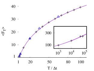
Figure 2: Numerical simulations for the average number of triangular facets on the convex hulls of some $3$-dimensional Lévy processes (with $10^{4}$ and $10^{3}$ sample paths’ realizations): standard Brownian motion (pluses), and a stable process with stability index $1.5$ (triangles). The solid line corresponds to the exact formula Eq. (III). The inset shows the asymptotics for large values of $T/\Delta t$, from Eq (14), with numerical simulations of 3-dimensional Brownian motion.

IV Conclusion

The exact formula established here for the average number of $(d-1)$-dimensional facets on the convex hull of a general $d$-dimensional Lévy process shows how universal certain aspects of the shape of spatial random processes are. Indeed this formula is valid not only for $d$-dimensional Brownian motion but for a vast class of Lévy processes, including all stable processes. This is reminiscent of the universality observed in the Sparre Andersen theorem Andersen (1954, 1955), to which the formula established here is linked via the arcsine and the uniform laws. To be more specific about the class of processes for which our formula holds: one needs the process to be truly $d$-dimensional and to have infinitely many increments on any time interval. This may not be the case for instance with compound Poisson processes. However, in many applications, one is dealing with Brownian motion or stable (self-similar) processes, which are covered here. Further work is needed to explore the cases not included, it may well be that they fall into the same universality class.

We will also seek to adapt the method introduced here to address multi-processes systems: what is the average number of facets on the global convex hull of $N$ independent spatial Brownian motions? One could also expect a large universality class in this context, and it will be of particular interest to see how the number of walkers intervenes on the $2\left[\ln\left(T/\Delta t\right)\right]^{d-1}$ asymptotics in the long time limit.

References

- Einstein (1905) A. Einstein, Annalen der Physik 322, 549 (1905).
- Chandrasekhar (1949) S. Chandrasekhar, Reviews of Modern Physics 21, 383 (1949).
- Viswanathan et al. (2011) G. Viswanathan, M. da Luz, E. Raposo, and H. Stanley, The Physics of Foraging: An Introduction to Random Searches and Biological Encounters (Cambridge University Press, 2011).
- Bénichou et al. (2005) O. Bénichou, M. Coppey, M. Moreau, P.-H. Suet, and R. Voituriez, Phys. Rev. Lett. 94, 198101 (2005).
- Havlin et al. (1991) S. Havlin, S. Buldyrev, H. Stanley, and G. Weiss, Journal of Physics A: Mathematical and General 24, L925 (1991).
- Edwards (1965) S. F. Edwards, Proc. Phys. Soc. 85, 613 (1965).
- De Gennes (1976) P. G. De Gennes, Macromolecules 9, 587 (1976).
- Westwater (1980) M. Westwater, Comm. Math. Phys. 72, 103 (1980).
- Doi and Edwards (1988) M. Doi and S. F. Edwards, The theory of polymer dynamics, International Series of Monographs on Physics (Oxford University Press, 1988).
- Worton (1987) B. Worton, Ecological Modelling 38, 277 (1987).
- Majumdar and Comtet (2004) S. N. Majumdar and A. Comtet, Phys. Rev. Lett. 92, 225501 (2004).
- Haber et al. (2000) C. Haber, S. A. Ruiz, and D. Wirtz, Proceedings of the National Academy of Sciences 97, 10792 (2000).
- Cook and Marenduzzo (2009) P. Cook and D. Marenduzzo, J. Cell. Biol. 188, 825 (2009).
- Takács (1980) L. Takács, Am. Math. Monthly 87, 142 (1980).
- El Bachir (1983) M. El Bachir, L’enveloppe convexe du mouvement brownien, Ph.D. thesis, Université Paul Sabatier, Toulouse, France (1983).
- Biane and Letac (2011) P. Biane and G. Letac, J. Theor. Prob. 24, 330 (2011).
- Cranston et al. (1989) M. Cranston, P. Hsu, and P. March, Annals Prob. 17, 144 (1989).
- Reymbaut et al. (2011) A. Reymbaut, S. N. Majumdar, and A. Rosso, J. Phys. A: Math. Theor. 44, 415001 (2011).
- Kampf et al. (2012) J. Kampf, G. Last, and I. Molchanov, Proc. Amer. Math. Soc. 140, 2527 (2012).
- Luković et al. (2013) M. Luković, T. Geisel, and S. Eule, New Jour. Phys. 15, 063034 (2013).
- Randon-Furling et al. (2009) J. Randon-Furling, S. N. Majumdar, and A. Comtet, Phys. Rev. Lett. 103, 140602 (2009).
- Chupeau et al. (2015a) M. Chupeau, O. Bénichou, and S. N. Majumdar, Physical Review E 91, 050104 (2015a).
- Chupeau et al. (2015b) M. Chupeau, O. Bénichou, and S. N. Majumdar, Physical Review E 92, 022145 (2015b).
- Kinney (1966) J. Kinney, Isr. J. Math. 4, 139 (1966).
- Randon-Furling (2009) J. Randon-Furling, Statistiques d’extrêmes du mouvement brownien et applications, Ph.D. thesis, Université Paris Sud-Paris XI (2009).
- Davydov (2012) Y. Davydov, Statistics and Probability Letters 82, 37 (2012).
- Eldan (2014) R. Eldan, Electron. J. Probab. 19, no. 45, 1 (2014).
- Molchanov and Wespi (2016) I. Molchanov and F. Wespi, Electron. Commun. Probab. 21, 11 pp. (2016).
- Rudnick and Gaspari (1987) J. Rudnick and G. Gaspari, Science 237, 384 (1987).
- Fougère and Desbois (1993) F. Fougère and J. Desbois, J. Phys. A: Math. Gen. 26, 7253 (1993).
- Alberts et al. (2002) B. Alberts, A. Johnson, and J. Lewis, “Molecular biology of the cell,” (Garland Science, New York, 2002) Chap. 3, 4th ed.
- Wilson et al. (2009) J. A. Wilson, A. Bender, T. Kaya, and P. A. Clemons, Journal of Chemical Information and Modeling 49, 2231 (2009).
- Holm and Sander (1993) L. Holm and C. Sander, Journal of Molecular Biology 233, 123 (1993).
- Meier et al. (1995) R. Meier, F. Ackermann, G. Herrmann, S. Posch, and G. Sagerer, in Proceedings., International Conference on Image Processing, Vol. 3 (1995) pp. 552–555 vol.3.
- Lee et al. (2006) M. Lee, P. Lloyd, X. Zhang, J. M. Schallhorn, K. Sugimoto, A. G. Leach, G. Sapiro, and K. N. Houk, The Journal of Organic Chemistry 71, 5082 (2006).
- Stout et al. (2008) M. Stout, J. Bacardit, J. D. Hirst, and N. Krasnogor, Bioinformatics 24, 916 (2008).
- Wang et al. (2006) Y. Wang, L.-Y. Wu, X.-S. Zhang, and L. Chen, “Automatic classification of protein structures based on convex hull representation by integrated neural network,” in Theory and Applications of Models of Computation: Third International Conference, TAMC 2006, Beijing, China, May 15-20, 2006. Proceedings, edited by J.-Y. Cai, S. B. Cooper, and A. Li (Springer Berlin Heidelberg, Berlin, Heidelberg, 2006) pp. 505–514.
- Badel-Chagnon et al. (1994) A. Badel-Chagnon, J. Nessi, L. Buffat, and S. Hazout, Journal of Molecular Graphics 12, 162 (1994).
- Coleman and Sharp (2006) R. G. Coleman and K. A. Sharp, Journal of Molecular Biology 362, 441 (2006).
- Randon-Furling (2014) J. Randon-Furling, Physical Review E 89, 052112 (2014).
- Fitzsimmons and Getoor (1995) P. Fitzsimmons and R. Getoor, Stochastic Processes and their Applications 58, 73 (1995).
- Knight (1996) F. Knight, Astérisque , 171 (1996).
- Kallenberg (1999) O. Kallenberg, Annals Prob. 27, 2011 (1999).
- Barndorff-Nielsen and Baxter (1963) O. Barndorff-Nielsen and G. Baxter, Transactions of the American Mathematical Society 108, 313 (1963).
- Kabluchko et al. (2016) Z. Kabluchko, V. Vysotsky, and D. Zaporozhets, arXiv preprint arXiv:1612.00249 (2016).
- Bertoin (1998) J. Bertoin, Lévy processes, Vol. 121 (Cambridge University Press, 1998).
- Dybiec et al. (2006) B. Dybiec, E. Gudowska-Nowak, and P. Hänggi, Physical Review E 73, 046104 (2006).
- Randon-Furling (2013) J. Randon-Furling, J. Phys. A: Math. Theor. 46, 015004 (2013).
- Maximon (2003) L. C. Maximon, in Proceedings of the Royal Society of London A: Mathematical, Physical and Engineering Sciences, Vol. 459 (The Royal Society, 2003) pp. 2807–2819.
- Zagier (2007) D. Zagier, in Frontiers in number theory, physics, and geometry II (Springer, 2007) pp. 3–65.
- Andersen (1954) E. S. Andersen, Mathematica Scandinavica , 263 (1954).
- Andersen (1955) E. S. Andersen, Mathematica Scandinavica , 195 (1955).