A Stabilized Cut Finite Element Method for the Darcy Problem on Surfaces

Peter Hansbo Department of Mechanical Engineering, Jönköping University, SE-55111 Jönköping, Sweden. peter.hansbo@ju.se Mats G. Larson  and  André Massing Department of Mathematics and Mathematical Statistics, Umeå University, SE-90187 Umeå, Sweden mats.larson@umu.se andre.massing@umu.se
Abstract.

We develop a cut finite element method for the Darcy problem on surfaces. The cut finite element method is based on embedding the surface in a three dimensional finite element mesh and using finite element spaces defined on the three dimensional mesh as trial and test functions. Since we consider a partial differential equation on a surface, the resulting discrete weak problem might be severely ill conditioned. We propose a full gradient and a normal gradient based stabilization computed on the background mesh to render the proposed formulation stable and well conditioned irrespective of the surface positioning within the mesh. Our formulation extends and simplifies the Masud-Hughes stabilized primal mixed formulation of the Darcy surface problem proposed in [28] on fitted triangulated surfaces. The tangential condition on the velocity and the pressure gradient is enforced only weakly, avoiding the need for any tangential projection. The presented numerical analysis accounts for different polynomial orders for the velocity, pressure, and geometry approximation which are corroborated by numerical experiments. In particular, we demonstrate both theoretically and through numerical results that the normal gradient stabilized variant results in a high order scheme.

Key words and phrases:
Surface PDE, Darcy Problem, cut finite element method, stabilization, condition number, a priori error estimates
2010 Mathematics Subject Classification:
Primary 65N30; Secondary 65N85, 58J05.

1. Introduction

1.1. Background and Earlier Work

In recent years, there has been a rapid development of cut finite element methods, also called trace finite element methods, for the numerical solution of partial differential equations (PDEs) on complicated or evolving surfaces embedded into $\mathbb{R}^{d}$. The main idea is to use the restriction of finite element basis functions defined on a $d$-dimensional background mesh to a discrete, piecewise smooth surface representation which is allowed to cut through the mesh in an arbitrary fashion. The active background mesh then consists of all elements which are cut by the discrete surface, and the finite element space restricted to the active mesh is used to discretize the surface PDE. This approach was first proposed in [32] for the Laplace-Beltrami on a closed surface, see also [3] and the references therein for an overview of cut finite element techniques.

Depending on the positioning of the discrete surface within the background mesh, the resulting system matrix might be severely ill conditioned and either preconditioning [31] or stabilization [4] is necessary to obtain a well conditioned linear system. The stabilization introduced and analyzed in [4] is based on so called face stabilization or ghost penalty, which provides control over the jump in the normal gradient across interior faces in the active mesh. In particular, it was shown that the condition number scaled in an optimal way, independent of how the surface cut the background mesh. Thanks its versatility, the face based stabilization can naturally be combined with discontinuous cut finite element methods as demonstrated in [7]. To reduce the matrix stencil and ease the implementation, a particular simple low order, full gradient stabilization using continuous piecewise linears was developed and analyzed in [8] for the Laplace-Beltrami operator. Then a unifying abstract framework for analysis of cut finite element methods on embedded manifolds of arbitrary codimension was developed in [6] and, in particular, the normal gradient stabilization term was introduced and analyzed. Further developments include convection problems [5, 33], coupled bulk-surface problems [9, 25] and higher order versions of trace fem for the Laplace-Beltrami operator [35, 23]. Moreover, extensions to time-dependent, parabolic-type problems on evolving domains were proposed in [27, 34].

So far, with their many applications to fluid dynamics, material science and biology, e.g., [21, 24, 30, 14, 15, 2], mainly scalar-valued, second order elliptic and parabolic type equations have been considered in the context of cut finite element methods for surface PDEs. Only very recently, vector-valued surface PDEs in combination with unfitted finite element technologies have been considered, for instance in the numerical discretization of surface-bulk problems modeling flow dynamics in fractured porous media [20, 10, 1, 19]. But while these contributions employed cut finite element type methods to discretize the bulk equations, only fitted (mixed and stabilized) finite elements methods on triangulated surfaces have been developed for vector surface equation such as the Darcy surface problem, see for instance [18, 28]. The present contribution is the first where a cut finite element method for a system of partial differential equations on a surfaces involving tangent vector fields of partial differential equations is developed.

1.2. New Contributions

We develop a stabilized cut finite element method for the numerical solution of the Darcy problem on a surface. The proposed variational formulation follows the approach in [28] for the Darcy problem on triangulated surfaces which is based on the stabilized primal mixed formulation by Masud and Hughes [29]. Note that standard mixed type elements are typically not available on discrete cut surfaces. Combining the ideas from [28] with the stabilized full gradient formulations of the Laplace-Beltrami problem from [8, 6], the tangent condition on both the velocity and the pressure gradient is enforced only weakly. When employing finite element function from the full $d$-dimensional background mesh, such a weak enforcement of the tangential condition is convenient and rather natural.

To render the proposed formulation stable and well conditioned irrespective of the relative surface position in the background mesh, we consider two stabilization forms: the full gradient stabilization introduced in [8] which is convenient for low order elements, and the normal gradient stabilization introduced in [6] which also works for higher order elements. Through these stabilizations, we gain control of the variation of the solution orthogonal to the surface, which in combination with the Masud-Hughes variational formulation results in a coercive formulation of the Darcy surface problem. In practice, the exact surface is approximated leading to a geometric error which we take into account in the error analysis. We show stability of the method and establish optimal order a priori error estimates. The presented numerical analysis also accounts for different polynomial orders for the velocity, pressure, and geometry approximation.

1.3. Outline

The paper is organized as follows: In Section 2 we present the Darcy problem on a surface together with its Masud-Hughes weak formulation, followed by the formulation of the cut finite element method in Section 3. In Section 4 we collect a number of preliminary theoretical results, which will be needed in Section 5 where the main a priori error estimates in the energy and $L^{2}$ norm are established. Finally, in Section 6 we present numerical results illustrating the theoretical findings of this work.

2. The Darcy Problem on a Surface

2.1. The Continuous Surface
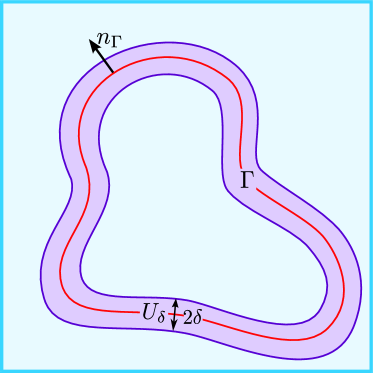
In what follows, $\Gamma$ denotes a smooth compact hypersurface without boundary which is embedded in ${{\mathbb{R}}}^{k}$ and equipped with a normal field $n:\Gamma\to\mathbb{R}^{d}$ and signed distance function $\rho$. Defining the tubular neighborhood of $\Gamma$ by $U_{\delta_{0}}(\Gamma)=\{x\in\mathbb{R}^{d}:\operatorname{dist}(x,\Gamma)<\delta_{0}\}$, the closest point projection $p(x)$ is the uniquely defined mapping given by

$\displaystyle p(x)=x-\rho(x)n(p(x))$ (2.1)

which maps $x\in U_{\delta_{0}}(\Gamma)$ to the unique point $p(x)\in\Gamma$ such that $|p(x)-x|=\operatorname{dist}(x,\Gamma)$ for some $\delta_{0}>0$, see [22]. The closest point projection allows the extension of a function $u$ defined on $\Gamma$ to its tubular neighborhood $U_{\delta_{0}}(\Gamma)$ using the pull back

$$u^{e}(x)=u\circ p(x)$$ (2.2)

In particular, we can smoothly extend the normal field $n_{\Gamma}$ to the tubular neighborhood $U_{\delta_{0}}(\Gamma)$. On the other hand, for any subset $\widetilde{\Gamma}\subseteq U_{\delta_{0}}(\Gamma)$ such that $p:\widetilde{\Gamma}\to\Gamma$ is bijective, a function $w$ on $\widetilde{\Gamma}$ can be lifted to $\Gamma$ by the push forward satisfying

$\displaystyle(w^{l})^{e}=w^{l}\circ p=w\quad\text{on }\widetilde{\Gamma}$ (2.3)

Finally, for any function space $V$ defined on $\Gamma$, we denote the space consisting of extended functions by $V^{e}$ and correspondingly, the notation $V^{l}$ refers to the lift of a function space $V$ defined on $\widetilde{\Gamma}$.

2.2. The Surface Darcy Problem

To formulate the Darcy problem on a surface, we first recall the definitions of the surface gradient and divergence. For a function $p:\Gamma\rightarrow\mathbb{R}$ the tangential gradient of $p$ can be expressed as

$$\nabla_{\Gamma}p={P_{\Gamma}}\nabla p^{e},$$ (2.4)

where $\nabla$ is the standard ${{\mathbb{R}}}^{d}$ gradient and ${P_{\Gamma}}={P_{\Gamma}}(x)$ denotes the orthogonal projection of $\mathbb{R}^{d}$ onto the tangent plane $T_{x}\Gamma$ of $\Gamma$ at $x\in\Gamma$ given by

$${P_{\Gamma}}=I-n\otimes n,$$ (2.5)

where $I$ is the identity matrix. Since $p^{e}$ is constant in the normal direction, we have the identity

$$\nabla p^{e}={P_{\Gamma}}\nabla p^{e}\quad\text{on $\Gamma$}.$$ (2.6)

Next, the surface divergence of a vector field $u:\Gamma\rightarrow\mathbb{R}^{d}$ is defined by

$$\operatorname{div}_{\Gamma}(u)=\text{tr}(u\otimes\nabla_{\Gamma})=\text{div}(u^{e})-n\cdot(u^{e}\otimes\nabla)\cdot n.$$ (2.7)

With these definitions, the Darcy problem on the surface $\Gamma$ is to seek the tangential velocity vector field $u_{t}:\Gamma\rightarrow T(\Gamma)$ and the pressure $p:\Gamma\rightarrow\mathbb{R}$ such that

$\displaystyle\operatorname{div}_{\Gamma}u_{t}$ $\displaystyle=f\qquad$ $\displaystyle\text{on $\Gamma$},$ (2.8a)
$\displaystyle u_{t}+\nabla_{\Gamma}p$ $\displaystyle=g\qquad$ $\displaystyle\text{on $\Gamma$}.$ (2.8b)

Here, $f:\Gamma\rightarrow\mathbb{R}$ is a given function such that $\int_{\Gamma}f=0$ and $g:\Gamma\rightarrow\mathbb{R}^{d}$ is a given tangential vector field.

2.3. The Masud-Hughes Weak Formulation

We follow [28] and base our finite element method on an extension of the Masud-Hughes weak formulation, originally proposed in [29] for planar domains, to the surface Darcy problem. Using Green’s formula

$$(\operatorname{div}_{\Gamma}v_{t},q)_{\Gamma}=-(v_{t},\nabla_{\Gamma}q)_{\Gamma}$$ (2.9)

valid for tangential vector fields $v_{t}$, a direct application of the original Masud-Hughes formulation is built upon the fact that the Darcy problem (2.8) solves the weak problem

$$a((u_{t},p),(v_{t},q))=l((v_{t},q))$$ (2.10)

for test functions $v\in[L^{2}(\Gamma)]$ and $q\in H^{1}(\Gamma)/\mathbb{R}$ with

$\displaystyle a((u_{t},p),(v_{t},q))$ $\displaystyle=(u_{t},v_{t})_{\Gamma}+(\nabla_{\Gamma}p,v_{t})_{\Gamma}-(u_{t},\nabla_{\Gamma}q)_{\Gamma}+\frac{1}{2}(u_{t}+\nabla_{\Gamma}p,-v_{t}+\nabla_{\Gamma}q)_{\Gamma}$ (2.11)
$\displaystyle l((v,q))$ $\displaystyle=(f,q)_{\Gamma}+(g,v_{t})_{\Gamma}+\frac{1}{2}(g,-v_{t}+\nabla_{\Gamma}q)_{\Gamma}$ (2.12)

As in [28] we enforce the tangent condition on the velocity weakly by using full velocity fields in formulation (2.10) and not only their tangential projection. But in contrast to [28] we also employ the identity (2.6) to replace the pressure related tangent gradients with the full gradient in order to simplify the implementation further. Earlier, such full gradient based formulation have been developed for the Poisson problem on the surface, see [35, 8]. With $\mathcal{V}=[L^{2}(\Gamma)]^{3}$ as the velocity space, $\mathcal{Q}=H^{1}(\Gamma)/\mathbb{R}$ as the pressure space and $\mathbb{V}=\mathcal{V}\times\mathcal{Q}$ as the total space, the resulting Masud-Hughes weak formulation of the Darcy surface problem (2.8) is to seek $U:=(u,p)\in\mathbb{V}$ satisfying

$$A(U,V)=L(V)\quad$$ (2.13)

for all $V:=(v,q)\in\mathbb{V}$, where

$\displaystyle A(U,V)$ $\displaystyle=(u,v)_{\Gamma}+(\nabla p,v)_{\Gamma}-(u,\nabla q)_{\Gamma}+\frac{1}{2}(u+\nabla p,-v+\nabla q)_{\Gamma},$ (2.14)
$\displaystyle L(V)$ $\displaystyle=(f,q)_{\Gamma}+(g,v)_{\Gamma}+\frac{1}{2}(g,-v+\nabla q)_{\Gamma}.$ (2.15)

Expanding the forms, the bilinear form $A$ and linear form $L$ can be rewritten as

$\displaystyle A(U,V)$ $\displaystyle=\frac{1}{2}(u,v)_{\Gamma}+\frac{1}{2}(\nabla p,\nabla q)_{\Gamma}+\frac{1}{2}(\nabla p,v)_{\Gamma}-\frac{1}{2}(u,\nabla q)_{\Gamma},$ (2.16)
$\displaystyle L(V)$ $\displaystyle=(f,q)_{\Gamma}+\frac{1}{2}(g,v+\nabla q)_{\Gamma}$ (2.17)

and consequently, the bilinear form $A$ consists of a symmetric positive definite part and a skew symmetric part. For a more detailed discussion on various weak formulation of the surface Darcy problem, we refer to [28]. Finally, note that since $\Gamma$ is smooth and $p\in Q$ is the solution to the elliptic problem $\operatorname{div}_{\Gamma}(\nabla_{\Gamma}p)=\operatorname{div}_{\Gamma}u_{t}-\operatorname{div}_{\Gamma}g=f-\operatorname{div}_{\Gamma}g$, the following elliptic regularity estimate holds

$$\|u_{t}\|_{H^{s+1}(\Gamma)}+\|p\|_{H^{s+2}(\Gamma)}\lesssim\|f\|_{H^{s}(\Gamma)}+\|g\|_{H^{s+1}(\Gamma)}$$ (2.18)

3. Cut Finite Element Methods for the Surface Darcy Problem

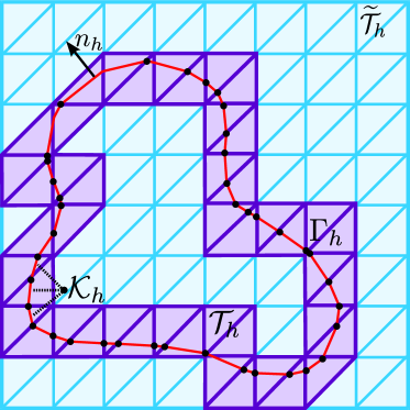
3.1. The Discrete Surface and Active Background Mesh

For $\Gamma$, we assume that the discrete surface approximation ${\Gamma_{h}}$ is represented by a piecewise smooth surface consisting of smooth $d-1$ dimensional surface parts $\mathcal{K}_{h}=\{K\}$ associated with a piecewise smooth normal field $n_{h}$. On $\Gamma_{h}=\bigcup_{K\in\mathcal{K}_{h}}K$ we can then define the discrete tangential projection ${P}_{\Gamma_{h}}$ as the pointwise orthogonal projection on the $d$-dimensional tangent space defined for each $x\in K$ and $K\in\mathcal{K}_{h}$. We assume that:

  • $\Gamma_{h}\subset U_{\delta_{0}}(\Gamma)$ and that the closest point mapping $p:\Gamma_{h}\rightarrow\Gamma$ is a bijection for $0<h\leq h_{0}$.

  • The following estimates hold

    $$\ \|\rho\|_{L^{\infty}(\Gamma_{h})}\lesssim h^{k_{g}+1},\qquad\|n^{e}-n_{h}\|_{L^{\infty}(\Gamma_{h})}\lesssim h^{k_{g}}.$$ (3.1)

Let $\widetilde{\mathcal{T}}_{h}$ be a quasi-uniform mesh, with mesh parameter $0<h\leq h_{0}$, which consists of shape regular closed simplices and covers some open and bounded domain $\Omega\subset\mathbb{R}^{k}$ containing the embedding neighborhood $U_{\delta_{0}}(\Gamma$). For the background mesh $\widetilde{\mathcal{T}}_{h}$ we define the active (background) $\mathcal{T}_{h}$ mesh

$\displaystyle\mathcal{T}_{h}$ $\displaystyle=\{T\in\widetilde{\mathcal{T}}_{h}:T\cap\Gamma_{h}\neq\emptyset\},$ (3.2)

see Figure 3.1 for an illustration. Finally, for the domain covered by $\mathcal{T}_{h}$ we introduce the notation

$\displaystyle N_{h}$ $\displaystyle=\cup_{T\in\mathcal{T}_{h}}T.$ (3.3)
Refer to caption
Refer to caption
Figure 3.1. Set-up of the continuous and discrete domains. (Left) Continuous surface $\Gamma$ enclosed by a $\delta$ tubular neighborhood $U_{\delta}(\Gamma)$. (Right) Discrete manifold $\Gamma_{h}$ embedded into a background mesh $\widetilde{\mathcal{T}}_{h}$ from which the active (background) mesh $\mathcal{T}_{h}$ is extracted.

3.2. Stabilized Cut Finite Element Methods

On the active mesh $\mathcal{T}_{h}$ we introduce the discrete space of continuous piecewise polynomials of order $k$,

$$X_{h}^{k}=\{v\in C(N_{h}):v|_{T}\in P_{k}(T)\;\forall\,T\in\mathcal{T}_{h}\}.$$ (3.4)

Occasionally, if the order is not of particular importance, we simply drop the superscript $k$. Next, the discrete velocity, pressure and total approximations spaces are defined by respectively

$\displaystyle\mathcal{V}_{h}=[X_{h}^{k_{u}}]^{d},\qquad\mathcal{Q}_{h}=\{v\in X_{h}^{k_{p}}:\lambda_{\Gamma_{h}}(v)=0\},\qquad\mathcal{W}_{h}=\mathcal{V}_{h}\times\mathcal{Q}_{h},$ (3.5)

where we explicitly permit different approximation orders $k_{u}$ and $k_{p}$ for the velocity and pressure space. As in the continuous case, $\lambda_{\Gamma_{h}}(\cdot)$ denotes the average operator on ${\Gamma_{h}}$ defined by $\lambda_{\Gamma_{h}}(v)=\tfrac{1}{{\Gamma_{h}}}\int_{\Gamma_{h}}v$. Now the stabilized, full gradient cut finite element method for the surface Darcy problem (2.8) is to seek $U_{h}:=(u_{h},p_{h})\in\mathbb{V}_{h}$ such that for all $V:=(v,p)\in\mathbb{V}_{h}$,

$\displaystyle B_{h}(U_{h},V)=L_{h}(V)$ (3.6)

where

$\displaystyle B_{h}(U_{h},V)$ $\displaystyle=A_{h}(U_{h},V)+S_{h}(U_{h},V)=L_{h}(V),$ (3.7)
$\displaystyle A_{h}(U_{h},V)$ $\displaystyle=(u_{h},v)_{{\Gamma_{h}}}+(\nabla p,v)_{{\Gamma_{h}}}-(u_{h},\nabla q)_{{\Gamma_{h}}}+\frac{1}{2}(u+\nabla p,-v+\nabla q)_{{\Gamma_{h}}},$ (3.8)
$\displaystyle S_{h}(U_{h},V)$ $\displaystyle=s_{h}(u_{h},v_{h})+s_{h}(p_{h},q_{h}),$ (3.9)
$\displaystyle L_{h}(V)$ $\displaystyle=(f,q)+\frac{1}{2}(g,v+\nabla q)_{\Gamma}.$ (3.10)

For the stabilization form $s_{h}$, two realizations will be proposed in this work. First, we consider a full gradient based stabilization originally introduced for Laplace-Beltrami surface problem in [8],

$\displaystyle s_{h}^{1}(u_{h},v_{h})$ $\displaystyle=h(\nabla u_{h},\nabla v_{h})_{\mathcal{T}_{h}},\qquad$ $\displaystyle s_{h}^{1}(p_{h},q_{h})=h(\nabla p_{h},\nabla q_{h})_{\mathcal{T}_{h}}.$ (3.11)
Second, to devise a higher order approximation scheme, the normal gradient stabilization
$\displaystyle s_{h}^{2}(u_{h},v_{h})$ $\displaystyle=h(n_{h}\cdot\nabla u_{h},n_{h}\cdot\nabla v_{h})_{\mathcal{T}_{h}},\qquad$ $\displaystyle s_{h}^{2}(p_{h},q_{h})=h(n_{h}\cdot\nabla p_{h},n_{h}\cdot\nabla q_{h})_{\mathcal{T}_{h}}$ (3.12)

first proposed and analyzed in [6] and then later also considered in [23], will be employed. In the remaining work, we will simply write $S_{h}$ and $s_{h}$ without superscripts as long as no distinction between the stabilization forms is needed.

Remark 3.1.

For the normal gradient stabilization, any $h$-scaling of the form $h^{\alpha-1}$ with $\alpha\in[0,2]$ gives an eglible stabilization operator, as pointed out in [6]. The condition $\alpha\leqslant 2$ guarantees that the stabilization result 4.1 for a properly scaled $L^{2}$ norm holds, the condition $\alpha\geqslant 0$ on the other hand assures that the condition number of the discrete linear system scales with the mesh size similar to the triangulated surface case. We refer to [6] for further details.

4. Preliminaries

To prepare the forthcoming analysis of the proposed cut finite element method in Section 5, we here collect and state a number of useful definitions, approximation results and estimates. In particular, we introduce suitable continuous and discrete norms, review the construction of a proper interpolation operator and recall the fundamental geometric estimates needed to quantify the quadrature errors introduced by the discretization of $\Gamma$.

4.1. Discrete Norms and Poincaré Inequalities

The symmetric parts of the bilinear forms $A$ and $A_{h}$ give raise to the following natural continuous and discrete “energy”-type norms

$\displaystyle|\mspace{-1.0mu}|\mspace{-1.0mu}|U|\mspace{-1.0mu}|\mspace{-1.0mu}|^{2}=\|u\|_{\Gamma}^{2}+\|\nabla p\|_{\Gamma}^{2},\qquad|\mspace{-1.0mu}|\mspace{-1.0mu}|U_{h}|\mspace{-1.0mu}|\mspace{-1.0mu}|_{h}^{2}=\|u_{h}\|_{{\Gamma_{h}}}^{2}+\|\nabla p_{h}\|_{{\Gamma_{h}}}^{2}+|U_{h}|_{S_{h}},$ (4.1)

where $|\cdot|_{S_{h}}$ denotes the semi-norm induced by the stabilization form $S_{h}$,

$\displaystyle|U_{h}|_{S_{h}}^{2}=S_{h}(U_{h},U_{h}).$ (4.2)

To show that $|\mspace{-1.0mu}|\mspace{-1.0mu}|\cdot|\mspace{-1.0mu}|\mspace{-1.0mu}|_{h}$ actually defines a proper norm, we recall the following result from [6].

Lemma 4.1.

For $v\in X_{h}$, the following estimate holds

$\displaystyle h^{-1}\|v\|^{2}_{\mathcal{T}_{h}}$ $\displaystyle\lesssim\|v\|_{\Gamma_{h}}^{2}+s_{h}^{i}(v,v)\quad\text{for }i=1,2,$ (4.3)

for $0<h\leq h_{0}$ with $h_{0}$ small enough.

Remark 4.2.

Simple counter examples show that the sole expression $\|v_{h}\|_{{\Gamma_{h}}}+\|\nabla q_{h}\|_{{\Gamma_{h}}}$ defines only a semi-norm on $\mathcal{V}_{h}\times\mathcal{Q}_{h}$. For instance, let $\Gamma=\{\phi=0\}$ be defined as the 00 level set of a smooth, scalar function $\phi$ such that $\nabla\phi\neq 0$ on $\Gamma$. Take $k_{u}=1$, $k_{p}=2$ and let ${\Gamma_{h}}=\{\phi_{h}=0\}$ where $\phi_{h}\in X_{h}^{1}$ is the Lagrange interpolant of $\phi$. Then $v_{h}=[\phi_{h}]^{d}\neq 0$ on $\mathcal{T}_{h}$ but clearly $\|v_{h}\|_{{\Gamma_{h}}}=0$. Defining $q_{h}=\phi_{h}^{2}\in\mathcal{Q}_{h}^{2}$ gives $\nabla q_{h}=2\phi_{h}\nabla\phi_{h}\neq 0$ but $\|\nabla q_{h}\|_{{\Gamma_{h}}}=0$ in this particular case.

Next, we state a simple surface-based discrete Poincaré estimate. For a proof we refer to [4].

Lemma 4.3.

Let $v\in X_{h}$, then it holds

$\displaystyle\|v-\lambda_{{\Gamma_{h}}}(v)\|_{\Gamma}\lesssim\|\nabla_{\Gamma_{h}}v\|_{{\Gamma_{h}}}$ (4.4)

for $0<h\leqslant h_{0}$ with $h_{0}$ chosen small enough.

Finally, the previous two lemma can be combined to obtain the following discrete Poincaré inequality for the discrete “energy” norm $|\mspace{-1.0mu}|\mspace{-1.0mu}|V|\mspace{-1.0mu}|\mspace{-1.0mu}|_{h}$.

Theorem 4.4.

For $(v,q)=V\in\mathbb{V}_{h}$, the following estimate holds

$\displaystyle h^{-1}\left(\|v\|^{2}_{\mathcal{T}_{h}}+\|q-\lambda_{\Gamma_{h}}(q)\|^{2}_{\mathcal{T}_{h}}\right)$ $\displaystyle\lesssim|\mspace{-1.0mu}|\mspace{-1.0mu}|V|\mspace{-1.0mu}|\mspace{-1.0mu}|_{h}$ (4.5)

for $0<h\leq h_{0}$ with $h_{0}$ small enough.

Refer to caption
Refer to caption
Figure 4.1. $L^{2}$ control mechanisms for the full gradient and normal gradient stabilization. (Left) While element $T_{1}$ has only a small intersection with $\Gamma_{h}$, there are several neighbor elements in $\mathcal{T}_{h}$ (purple) which share the node $x_{0}$ and have a “fat” intersection with $\Gamma_{h}$. The appearance of the full gradient in stabilization $s_{h}^{1}$ allows to integrate along arbitrary directions and thus gives raise to the control of $\|v\|_{T_{1}}$ through Lemma 4.1. (Right) The fat intersection property for the discrete “normal” tube guarantees that still a significant portion of $T_{1}$ can be reached when integrating along normal-like paths which start from $\Gamma_{h}$ and which reside completely inside $\mathcal{T}_{h}$.

4.2. Trace Estimates and Inverse Inequalities

First, we recall the following trace inequality for $v\in H^{1}(\mathcal{T}_{h})$

$$\|v\|_{\partial T}\lesssim h^{-1/2}\|v\|_{T}+h^{1/2}\|\nabla v\|_{T}\quad\forall\,T\in\mathcal{T}_{h},$$ (4.6)

while for the intersection $\Gamma\cap T$ the corresponding inequality

$\displaystyle\|v\|_{\Gamma\cap T}\lesssim h^{-1/2}\|v\|_{T}+h^{1/2}\|\nabla v\|_{T}\quad\forall\,T\in\mathcal{T}_{h}$ (4.7)

holds whenever $h$ is small enough, see [26] for a proof. In the following, we will also need some well-known inverse estimates for $v_{h}\in V_{h}$:

$$\displaystyle\|\nabla v_{h}\|_{T}\lesssim h^{-1}\|v_{h}\|_{T}\quad\forall\,T\in\mathcal{T}_{h},$$ (4.8)
$$\displaystyle\|v_{h}\|_{\partial T}\lesssim h^{-1/2}\|v_{h}\|_{T},\qquad\|\nabla v_{h}\|_{\partial T}\lesssim h^{-1/2}\|\nabla v_{h}\|_{T}\quad\forall\,T\in\mathcal{T}_{h},$$ (4.9)

and the following “cut versions” when $K\cap T\not\subseteq\partial T$

$\displaystyle\|v_{h}\|_{K\cap T}$ $\displaystyle\lesssim h^{-1/2}\|v_{h}\|_{T},$ $\displaystyle\qquad\|\nabla v_{h}\|_{K\cap T}$ $\displaystyle\lesssim h^{-1/2}\|\nabla v_{h}\|_{T}$ $\displaystyle\quad\forall\,K\in\mathcal{K}_{h},\;\forall\,T\in\mathcal{T}_{h},$ (4.10)

which are an immediate consequence of similar inverse estimates presented in [26].

4.3. Geometric Estimates

We now summarize some standard geometric identities and estimates which typically are used in the numerical analysis of surface PDE discretizations when passing from the discrete surface to the continuous one and vice versa. For a detailed derivation, we refer to [12, 32, 11, 13, 7]. Starting with the Hessian of the signed distance function

$\displaystyle\mathcal{H}=\nabla\otimes\nabla\rho\quad\text{on }U_{\delta_{0}}(\Gamma),$ (4.11)

the derivative of the closest point projection and of an extended function $v^{e}$ is given by

$$\displaystyle Dp={P_{\Gamma}}(I-\rho\mathcal{H})={P_{\Gamma}}-\rho\mathcal{H},$$ (4.12)
$$\displaystyle Dv^{e}=D(v\circ p)=DvDp=DvP_{\Gamma}(I-\rho\mathcal{H}).$$ (4.13)

The self-adjointness of ${P_{\Gamma}}$, ${P}_{\Gamma_{h}}$, and $\mathcal{H}$, and the fact that ${P_{\Gamma}}\mathcal{H}=\mathcal{H}=\mathcal{H}{P_{\Gamma}}$ and ${P_{\Gamma}}^{2}={P_{\Gamma}}$ then leads to the identities

$\displaystyle\nabla v^{e}$ $\displaystyle={P_{\Gamma}}(I-\rho\mathcal{H})\nabla v={P_{\Gamma}}(I-\rho\mathcal{H})\nabla_{\Gamma}v,$ (4.14)
$\displaystyle\nabla_{\Gamma_{h}}v^{e}$ $\displaystyle={P}_{\Gamma_{h}}(I-\rho\mathcal{H}){P_{\Gamma}}\nabla v=B^{T}\nabla_{\Gamma}v,$ (4.15)

where the invertible linear mapping

$\displaystyle B=P_{\Gamma}(I-\rho\mathcal{H})P_{\Gamma_{h}}:T_{x}({\Gamma_{h}})\to T_{p(x)}(\Gamma)$ (4.16)

maps the tangential space of $\Gamma_{h}$ at $x$ to the tangential space of $\Gamma$ at $p(x)$. Setting $v=w^{l}$ and using the identity $(w^{l})^{e}=w$, we immediately get that

$\displaystyle\nabla_{\Gamma}w^{l}=B^{-T}\nabla_{\Gamma_{h}}w$ (4.17)

for any elementwise differentiable function $w$ on $\Gamma_{h}$ lifted to $\Gamma$. We recall from [22, Lemma 14.7] that for $x\in U_{\delta_{0}}(\Gamma)$, the Hessian $\mathcal{H}$ admits a representation

$$\mathcal{H}(x)=\sum_{i=1}^{k}\frac{\kappa_{i}^{e}}{1+\rho(x)\kappa_{i}^{e}}a_{i}^{e}\otimes a_{i}^{e},$$ (4.18)

where $\kappa_{i}$ are the principal curvatures with corresponding principal curvature vectors $a_{i}$. Thus

$$\|\mathcal{H}\|_{L^{\infty}(U_{\delta_{0}}(\Gamma))}\lesssim 1$$ (4.19)

for $\delta_{0}>0$ small enough. In the course of the a priori analysis in Section 5, we will need to estimate various operator compositions involving $B$, the continuous and discrete tangential and normal projection operators. More precisely, using the definition ${Q}_{\Gamma_{h}}:=I-{P}_{\Gamma_{h}}=n_{h}\otimes n_{h}$, the following bounds will be employed at several occasions.

Lemma 4.5.
$\displaystyle\|{P_{\Gamma}}-{P_{\Gamma}}{P}_{\Gamma_{h}}{P_{\Gamma}}\|_{L^{\infty}(\Gamma)}$ $\displaystyle\lesssim h^{2k_{g}},\qquad$ $\displaystyle\|{Q}_{\Gamma_{h}}{P_{\Gamma}}\|_{L^{\infty}(\Gamma)}$ $\displaystyle\lesssim h^{k_{g}},\qquad$ $\displaystyle\|{P_{\Gamma}}{Q}_{\Gamma_{h}}\|_{L^{\infty}({\Gamma_{h}})}$ $\displaystyle\lesssim h^{k_{g}},$ (4.20)
$\displaystyle\|B\|_{L^{\infty}(\Gamma_{h})}$ $\displaystyle\lesssim 1,\qquad$ $\displaystyle\|B^{-1}\|_{L^{\infty}(\Gamma)}$ $\displaystyle\lesssim 1,\qquad$ $\displaystyle\|P_{\Gamma}-BB^{T}\|_{L^{\infty}(\Gamma)}$ $\displaystyle\lesssim h^{k_{g}+1}.$ (4.21)
Proof.

All these estimate have been proved earlier, see [12, 13, 8] and we only include a short proof for the reader’s convenience. We start with the bounds summarized in (4.20). An easy calculation shows that ${P_{\Gamma}}-{P_{\Gamma}}{P}_{\Gamma_{h}}{P_{\Gamma}}={P_{\Gamma}}({P_{\Gamma}}-{P}_{\Gamma_{h}})^{2}{P_{\Gamma}}$ from which the desired bound follows by observing that ${P_{\Gamma}}-{P}_{\Gamma_{h}}=(n-n_{h})\otimes n+n_{h}\otimes(n-n_{h})$ and thus $\|({P_{\Gamma}}-{P}_{\Gamma_{h}})^{2}\|_{L^{\infty}(\Gamma_{h})}\lesssim\|n-n_{h}\|_{L^{\infty}(\Gamma_{h})}^{2}\lesssim h^{2k_{g}}.$ Next, observe that

$\displaystyle\|{Q}_{\Gamma_{h}}{P_{\Gamma}}\|_{L^{\infty}(\Gamma)}$ $\displaystyle=\|n_{h}\otimes n_{h}-(n_{h},n)_{\mathbb{R}^{d}}n_{h}\otimes n\|_{L^{\infty}(\Gamma)}$ (4.22)
$\displaystyle=\|(1-(n_{h},n)_{\mathbb{R}^{d}})n_{h}\otimes n_{h}\|_{L^{\infty}(\Gamma)}+\|(n_{h},n)_{\mathbb{R}^{d}}n_{h}\otimes(n_{h}-n)\|_{L^{\infty}(\Gamma)}$ (4.23)
$\displaystyle\lesssim h^{2k_{g}}+h^{k_{g}}.$ (4.24)

Turning to (4.21), the first two bounds follow directly from (4.16) and  (4.19) together with the assumption $\|\rho\|_{L^{\infty}(\Gamma_{h})}\lesssim h^{k_{g}+1}$. Finally, unwinding the definition of $B$, we find that ${P_{\Gamma}}-BB^{T}={P_{\Gamma}}-{P_{\Gamma}}{P}_{\Gamma_{h}}{P_{\Gamma}}+O(h^{k_{g}+1}),$ which together with the previously derived estimate for ${P_{\Gamma}}-{P_{\Gamma}}{P}_{\Gamma_{h}}{P_{\Gamma}}$ gives the stated operator bound. ∎

The previous lemma allows us to quantify the error introduced by using the full gradient in (3.8) instead of $\nabla_{\Gamma_{h}}$. To do so we decompose the full gradient as $\nabla=\nabla_{\Gamma_{h}}+{Q}_{\Gamma_{h}}\nabla$ with ${Q}_{\Gamma_{h}}=I-{P}_{\Gamma_{h}}=n_{h}\otimes n_{h}$. We then have

Corollary 4.6.

For $v\in H^{1}(\Gamma)$ and $w\in V_{h}$ it holds

$\displaystyle\|{Q}_{\Gamma_{h}}\nabla v^{e}\|_{\Gamma_{h}}\lesssim h^{k_{g}}\|\nabla_{\Gamma}v\|_{\Gamma},\qquad\|{P_{\Gamma}}{Q}_{\Gamma_{h}}\nabla w\|_{\Gamma_{h}}\lesssim h^{k_{g}}\|\nabla w\|_{\Gamma_{h}}.$ (4.25)
Proof.

Since $\|{Q}_{\Gamma_{h}}{P_{\Gamma}}\|_{L^{\infty}(\Gamma_{h})}\lesssim h^{k_{g}}$, the first estimate follows directly from the identity $\nabla v^{e}$ = ${P_{\Gamma}}(I-\rho\mathcal{H})\nabla_{\Gamma}v$ from (4.14), while the second estimate is a immediate consequence of (4.20). ∎

Next, for a subset $\omega\subset{\Gamma_{h}}$, we have the change of variables formula

$$\int_{\omega^{l}}g^{l}d\Gamma=\int_{\omega}g|B|d\Gamma_{h}$$ (4.26)

with $|B|$ denoting the absolute value of the determinant of $B$. The determinant $|B|$ satisfies the following estimates.

Lemma 4.7.

It holds

$\displaystyle\|1-|B|\|_{L^{\infty}(\mathcal{K}_{h})}$ $\displaystyle\lesssim h^{k_{g}+1},$ $\displaystyle\qquad\||B|\|_{L^{\infty}(\mathcal{K}_{h})}$ $\displaystyle\lesssim 1,$ $\displaystyle\qquad\||B|^{-1}\|_{L^{\infty}(\mathcal{K}_{h})}$ $\displaystyle\lesssim 1.$ (4.27)

Combining the various estimates for the norm and the determinant of $B$ shows that for $m=0,1$

$\displaystyle\|v\|_{H^{m}(\mathcal{K}_{h}^{l})}$ $\displaystyle\sim\|v^{e}\|_{H^{m}(\mathcal{K}_{h})}$ $\displaystyle\quad\text{for }v\in H^{m}(\mathcal{K}_{h}^{l}),$ (4.28)
$\displaystyle\|w^{l}\|_{H^{m}(\mathcal{K}_{h}^{l})}$ $\displaystyle\sim\|w\|_{H^{m}(\mathcal{K}_{h})}$ $\displaystyle\quad\text{for }w\in V_{h}.$ (4.29)

Next, we observe that thanks to the coarea-formula (cf. Evans and Gariepy [17])

$\displaystyle\int_{U_{\delta}}f(x)\,dx=\int_{-\delta}^{\delta}\left(\int_{\Gamma(r)}f(y,r)\,\mathrm{d}\Gamma_{r}(y)\right)\,\mathrm{d}r,$

the extension operator $v^{e}$ defines a bounded operator $H^{m}(\Gamma)\ni v\mapsto v^{e}\in H^{m}(U_{\delta}(\Gamma))$ satisfying the stability estimate

$\displaystyle\|v^{e}\|_{k,U_{\delta}(\Gamma)}\lesssim\delta^{1/2}\|v\|_{k,\Gamma},\qquad 0\leqslant k\leqslant m$ (4.30)

for $0<\delta\leqslant\delta_{0}$, where the hidden constant depends only on the curvature of $\Gamma$.

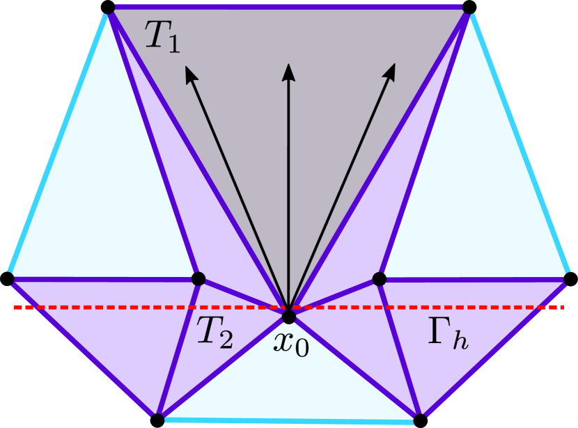
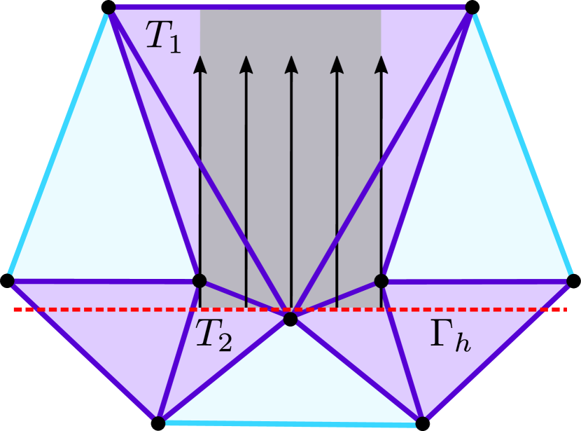
4.4. Interpolation Operator

Next, we recall from [16] that for $v\in H^{k+1}(N_{h})$, the Clément interpolant $\pi_{h}:L^{2}(\mathcal{T}_{h})\rightarrow X_{h}^{k}$ satisfies the local interpolation estimates

$\displaystyle\|v-\pi_{h}v\|_{m,T}$ $\displaystyle\lesssim h^{k+1-m}|v|_{k+1,\omega(T)},$ $\displaystyle\quad 0\leqslant m\leqslant k+1,\quad$ $\displaystyle\forall\,T\in\mathcal{T}_{h},$ (4.31)

where $\omega(T)$ consists of all elements sharing a vertex with $T$. Now with the help of the extension operator $(\cdot)^{e}$, an interpolation operator $\pi_{h}:L^{2}(\Gamma)\to X^{k}_{h}$ can be constructed by setting $\pi_{h}v=\pi_{h}v^{e}$, where we took the liberty of using the same symbol. The resulting interpolation operator satisfies the following error estimate.

Lemma 4.8.

For $V=(v,p)\in[H^{k_{u}}(\Gamma)]^{d}\times H^{k_{p}+1}(\Gamma)$ and $k_{u},k_{p}\geqslant 1$, the interpolant defined by $\Pi_{h}V^{e}=(\pi_{h}v^{e},\pi_{h}q^{e})\in\mathcal{V}_{h}^{k_{u}}\times\mathcal{Q}_{h}^{k_{p}}$ satisfies the interpolation estimate

$\displaystyle|\mspace{-1.0mu}|\mspace{-1.0mu}|V^{e}-\Pi_{h}V^{e}|\mspace{-1.0mu}|\mspace{-1.0mu}|_{h}\lesssim h^{k_{u}}\|v\|_{k_{u},\Gamma}+h^{k_{p}}\|q\|_{k_{p}+1,\Gamma}.$ (4.32)
Proof.

Choosing $\delta_{0}\sim h$, it follows directly from combining the trace inequality (4.7), the interpolation estimate (4.31), and the stability estimate (4.30) that the first two terms in the definition of $|\mspace{-1.0mu}|\mspace{-1.0mu}|V^{e}-\Pi_{h}V^{e}|\mspace{-1.0mu}|\mspace{-1.0mu}|_{h}^{2}=\|v^{e}-\pi_{h}v^{e}\|_{\Gamma}^{2}+\|\nabla(p^{e}-\pi_{h}p^{e})\|_{\Gamma}^{2}+|V^{e}-\Pi_{h}V^{e}|_{S_{h}}^{2}$ satisfies the desired estimate. Since $|\cdot|_{S_{h}^{2}}\leqslant|\cdot|_{S_{h}^{1}}$ it is enough to focus on the full gradient stabilization $S_{h}=S_{h}^{1}$ for the remaining part. With the same chain of estimates we find that

$\displaystyle|V^{e}-\Pi_{h}V^{e}|_{S_{h}}^{2}$ $\displaystyle=h\bigl{(}\|\nabla(v^{e}-\pi_{h}v^{e})\|_{\mathcal{T}_{h}}^{2}+\|\nabla(p^{e}-\pi_{h}p^{e})\|_{\mathcal{T}_{h}}^{2}\bigr{)}$ (4.33)
$\displaystyle\lesssim h^{2k_{u}-1}\|v^{e}\|_{k_{u},\mathcal{T}_{h}}^{2}+h^{2k_{p}+1}\|q^{e}\|_{k_{p}+1,\mathcal{T}_{h}}^{2}$ (4.34)
$\displaystyle\lesssim h^{2k_{u}}\|v\|_{k_{u},\Gamma}^{2}+h^{2k_{p}+2}\|q\|_{k_{p}+1,\Gamma}^{2}$ (4.35)

which concludes the proof. ∎

5. A Priori Error Estimates

We now state and prove the main a priori error estimates for the stabilized cut finite element method (3.6). The proofs rest upon a Strang-type lemma splitting the total error into an interpolation error, a consistency error arising from the additional stabilization term $S_{h}$ and finally, a geometric error caused by the discretization of the surface. We start with establishing suitable estimates for the consistency and quadrature error before we present the final a priori error estimates at the end of this section.

5.1. Estimates for the Quadrature and Consistency Error

The purpose of the next lemma is two-fold. First, it shows that the full gradient stabilization will not affect the expected convergence order when low-order elements are used. Second, it demonstrates that only the normal gradient stabilization is suitable for high order discretizations where the geometric approximation order $k_{g}$ needs to satisfy $k_{g}>1$.

Lemma 5.1.

Let $U=(u,p)\in[H^{1}(\Gamma)]^{d}_{t}\times H^{1}(\Gamma)$. Then it holds

$\displaystyle|U^{e}|_{S_{h}^{1}}$ $\displaystyle\lesssim h(\|\nabla_{\Gamma}u\|_{\Gamma}+\|\nabla_{\Gamma}p\|_{\Gamma}),$ (5.1)
$\displaystyle|U^{e}|_{S_{h}^{2}}$ $\displaystyle\lesssim h^{k_{g}+1}(\|\nabla_{\Gamma}u\|_{\Gamma}+\|\nabla_{\Gamma}p\|_{\Gamma}).$ (5.2)
Proof.

A simple application of stability estimate (4.30) with $\delta\sim h$ shows that for $S_{h}^{1}$,

$\displaystyle S_{h}^{1}(U^{e},U^{e})=h\|\nabla u^{e}\|_{\mathcal{T}_{h}}^{2}+h\|\nabla p^{e}\|_{\mathcal{T}_{h}}^{2}\lesssim h^{2}(\|u\|_{1,\Gamma}^{2}+\|p\|_{1,\Gamma}^{2}).$ (5.3)

Turning to $S_{h}^{2}$, the pressure part of the normal gradient stabilization can be estimated by

$\displaystyle s_{p}(p^{e},p^{e})=h\|{Q}_{\Gamma_{h}}\nabla p^{e}\|_{\mathcal{T}_{h}}^{2}=h\|({Q}_{\Gamma_{h}}-{Q_{\Gamma}})\nabla p^{e}\|_{\mathcal{T}_{h}}^{2}\lesssim h^{2k_{g}+1}\|\nabla p^{e}\|_{\mathcal{T}_{h}}^{2}\lesssim h^{2k_{g}+2}\|\nabla_{\Gamma}p\|_{\Gamma}^{2},$ (5.4)

and similarly, $|u^{e}|_{s_{h}^{2}}\lesssim h^{k_{g}+1}\|\nabla_{\Gamma}u\|_{\Gamma}$ for $u\in[H^{1}(\Gamma)]^{d}$. ∎

Lemma 5.2.

Let $U=(u,p)\in[L^{2}(\Gamma)]_{t}^{d}\times H^{1}(\Gamma)/\mathbb{R}$ be the solution to weak problem (2.10) and assume that $V\in\mathbb{V}_{h}$. Then

$\displaystyle|L(V^{l})-L_{h}(V)|+|A(U,V^{l})-A_{h}(U^{e},V_{h})|$ $\displaystyle\lesssim h^{k_{g}}(\|f\|_{\Gamma}+\|g\|_{\Gamma})|\mspace{-1.0mu}|\mspace{-1.0mu}|V|\mspace{-1.0mu}|\mspace{-1.0mu}|_{h}.$ (5.5)

Furthermore, if $\Phi=(\phi_{u},\phi_{p})\in[H^{1}(\Gamma)]^{d}_{t}\times H^{2}(\Gamma)/\mathbb{R}$ and $\Phi_{h}:=\Pi_{h}\Phi=(\pi_{h}\phi_{u},\pi_{h}\phi_{p})$, we have the improved estimate

$\displaystyle|L(\Phi_{h}^{l})-L_{h}(\Phi_{h})|+|A(U,\Phi_{h}^{l})-A_{h}(U^{e},\Phi_{h})|$ $\displaystyle\lesssim h^{k_{g}+1}(\|f\|_{\Gamma}+\|g\|_{\Gamma})(\|\phi_{u}\|_{1,\Gamma}+\|\phi_{p}\|_{2,\Gamma}).$ (5.6)
Proof.

We start with the term $L(\cdot)-L_{h}(\cdot)$. Unwinding the definition of the linear forms $L$ and $L_{h}$, we get

$\displaystyle L(V^{l})-L_{h}(V)$ $\displaystyle=\Bigl{(}(f,q^{l})_{\Gamma}-(f^{e},q)_{\Gamma_{h}}+\frac{1}{2}\left((g,v^{l})_{\Gamma}-(g^{e},v)_{\Gamma_{h}}\right)\Bigr{)}$ (5.7)
$\displaystyle\quad+\frac{1}{2}\left((g,\nabla q^{l})_{\Gamma}-(g^{e},\nabla q)_{\Gamma_{h}}\right)=I+II.$ (5.8)

For the first term, a change of variables together with estimate (4.27) for the determinant $|B|$ yields

$\displaystyle I$ $\displaystyle=(f,(1-|B|^{-1})q^{l})_{\Gamma}+\frac{1}{2}(g,(1-|B|^{-1})v^{l})_{\Gamma}$ (5.9)
$\displaystyle\lesssim h^{k_{g}+1}\left(\|f\|_{\Gamma}+\|g\|_{\Gamma}\right)(\|q^{l}\|_{\Gamma}+\|v^{l}\|_{\Gamma})$ (5.10)
$\displaystyle\lesssim h^{k_{g}+1}\left(\|f\|_{\Gamma}+\|g\|_{\Gamma}\right)|\mspace{-1.0mu}|\mspace{-1.0mu}|V|\mspace{-1.0mu}|\mspace{-1.0mu}|_{h},$ (5.11)

where in the last step, we used the norm equivalences (4.29) and the discrete Poincaré inequality (4.4) to pass to $|\mspace{-1.0mu}|\mspace{-1.0mu}|V_{h}|\mspace{-1.0mu}|\mspace{-1.0mu}|_{h}$. To estimate $II$, we split $\nabla q$ into its tangential and normal part

$\displaystyle\nabla q=\nabla_{\Gamma_{h}}q+{Q}_{\Gamma_{h}}\nabla q.$ (5.12)

Note that for the tangential field $g$, the identities

$\displaystyle(g,\nabla q^{l})_{\Gamma}=(g,\nabla_{\Gamma}q^{l})_{\Gamma},\quad(g^{e},\nabla q)_{\Gamma_{h}}=({P_{\Gamma}}g^{e},\nabla q)_{{\Gamma_{h}}}$ (5.13)

hold and thus using ${P_{\Gamma}}g=g$ once more and the fact that ${P_{\Gamma}}^{T}={P_{\Gamma}}$ allows us to rewrite $II$ as

$\displaystyle 2II$ $\displaystyle=(g,\nabla_{\Gamma}q^{l})_{\Gamma}-(g^{e},\nabla_{\Gamma_{h}}q)_{\Gamma_{h}}-(g^{e},{Q}_{\Gamma_{h}}\nabla q)_{\Gamma_{h}}$ (5.14)
$\displaystyle=(g,({P_{\Gamma}}-|B|^{-1}B^{T})\nabla_{\Gamma}q^{l})_{\Gamma}-({P_{\Gamma}}g^{e},{Q}_{\Gamma_{h}}\nabla q)_{{\Gamma_{h}}}$ (5.15)
$\displaystyle=(g,{P_{\Gamma}}({P_{\Gamma}}-|B|^{-1}B^{T})\nabla_{\Gamma}q^{l})_{\Gamma}+(g^{e},{P_{\Gamma}}{Q}_{\Gamma_{h}}\nabla q)_{{\Gamma_{h}}}$ (5.16)
$\displaystyle=II_{t}+II_{n}.$ (5.17)

Unwinding the definition of $B$ given in (4.16) together with the estimates for the determinant $|B|$ from Lemma 4.7 reveals that

$\displaystyle{P_{\Gamma}}({P_{\Gamma}}-|B|^{-1}B^{T})$ $\displaystyle={P_{\Gamma}}({P_{\Gamma}}-B^{T})+{P_{\Gamma}}(|B|^{-1}-1)B^{T}$ (5.18)
$\displaystyle\sim{P_{\Gamma}}({P_{\Gamma}}-{P}_{\Gamma_{h}}(I-\rho\mathcal{H}){P_{\Gamma}})+h^{k_{g}+1}$ (5.19)
$\displaystyle\sim{P_{\Gamma}}-{P_{\Gamma}}{P}_{\Gamma_{h}}{P_{\Gamma}}+h^{k_{g}+1}.$ (5.20)

Consequently, using the bounds for ${P_{\Gamma}}-{P_{\Gamma}}{P}_{\Gamma_{h}}{P_{\Gamma}}$ and ${P_{\Gamma}}{Q}_{\Gamma_{h}}$ from Lemma 4.5, we deduce that

$\displaystyle II_{t}$ $\displaystyle\lesssim h^{k_{g}+1}\|g\|_{\Gamma}\|\nabla_{\Gamma}q^{l}\|_{\Gamma}\lesssim h^{k_{g}+1}\|g\|_{\Gamma}|\mspace{-1.0mu}|\mspace{-1.0mu}|V|\mspace{-1.0mu}|\mspace{-1.0mu}|_{h},$ (5.21)
$\displaystyle II_{n}$ $\displaystyle\lesssim h^{k_{g}}\|g\|_{\Gamma}\|\nabla q\|_{{\Gamma_{h}}}\lesssim h^{k_{g}}\|g\|_{\Gamma}|\mspace{-1.0mu}|\mspace{-1.0mu}|V|\mspace{-1.0mu}|\mspace{-1.0mu}|_{h}.$ (5.22)

In the special case $q=\pi_{h}\phi_{p}^{e}$, the bound for $II_{n}$ can be further improved to

$\displaystyle II_{n}$ $\displaystyle=(g^{e},{P_{\Gamma}}{Q}_{\Gamma_{h}}{P_{\Gamma}}\nabla\phi_{p}^{e})_{{\Gamma_{h}}}+(g^{e},{P_{\Gamma}}{Q}_{\Gamma_{h}}\nabla(\pi_{h}\phi_{p}^{e}-\phi_{p}^{e}))_{{\Gamma_{h}}},$ (5.23)
$\displaystyle\lesssim h^{k_{g}+1}\|g\|_{\Gamma}\|\nabla\phi_{p}\|_{\Gamma}+h^{k_{g}+1}\|g\|_{\Gamma}\|\phi_{p}\|_{2,\Gamma},$ (5.24)

where we once more employed the identity $\nabla\phi_{p}^{e}={P_{\Gamma}}\nabla\phi_{p}^{e}$, the estimates (4.20) for the operators ${P_{\Gamma}}{Q}_{\Gamma_{h}}{P_{\Gamma}}$ and ${P_{\Gamma}}{Q}_{\Gamma_{h}}$ and finally, the interpolation estimate (4.32).

Turning to the term $A(U,\cdot)-A(U^{e},\cdot)$ in (5.5) and (5.6) and recalling the definition of bilinear forms $A$ and $A_{h}$, we rearrange terms to obtain

$\displaystyle 2\left(A(U,V^{l})-A_{h}(U^{e},V)\right)$ $\displaystyle=\left((u,v^{l})_{\Gamma}-(u^{e},v)_{\Gamma_{h}}\right)+\left((\nabla p,v^{l})_{\Gamma}-(\nabla p^{e},v)_{{\Gamma_{h}}}\right)$ (5.25)
$\displaystyle\quad-\left((u,\nabla q^{l})_{\Gamma}-(u^{e},\nabla q)_{{\Gamma_{h}}}\right)+\left((\nabla p,\nabla q^{l})_{\Gamma}-(\nabla p^{e},\nabla q)_{\Gamma_{h}}\right)$ (5.26)
$\displaystyle=I+II-III+IV.$ (5.27)

To estimate the term $I$ $IV$, we proceed along the same lines as in the previous part. As before, the first term can be bounded as follows

$\displaystyle I$ $\displaystyle=(u,(1-|B|^{-1})v^{l})_{\Gamma}\lesssim h^{k_{g}+1}\|u\|_{\Gamma}\|v^{l}\|_{\Gamma}\lesssim h^{k_{g}+1}\|u\|_{\Gamma}|\mspace{-1.0mu}|\mspace{-1.0mu}|V|\mspace{-1.0mu}|\mspace{-1.0mu}|_{h}.$ (5.28)

For the remaining terms, the appearance of the full gradient necessitates a similar split into its normal and tangential part as before, followed by a lifting of the tangential part and the use of the operator estimates (4.20) and (4.21). Recall that $\nabla p=\nabla_{\Gamma}p^{e}$ and consequently,

$\displaystyle II$ $\displaystyle=(\nabla_{\Gamma}p,v^{l})_{\Gamma}-(\nabla_{\Gamma_{h}}p^{e},v)_{{\Gamma_{h}}}-({Q}_{\Gamma_{h}}\nabla p^{e},v)_{{\Gamma_{h}}}$ (5.29)
$\displaystyle=(({P_{\Gamma}}-|B|^{-1}B^{T})\nabla_{\Gamma}p,v^{l})_{\Gamma}-({Q}_{\Gamma_{h}}{P_{\Gamma}}\nabla p^{e},v)_{{\Gamma_{h}}}$ (5.30)
$\displaystyle=II_{t}+II_{n}.$ (5.31)

Now expand $B$ to see that ${P_{\Gamma}}-|B|^{-1}B^{T}\sim{P_{\Gamma}}-{P}_{\Gamma_{h}}{P_{\Gamma}}+h^{k_{g}+1}\sim{Q}_{\Gamma_{h}}{P_{\Gamma}}+h^{k_{g}+1}$ and apply the operator bounds from Lemma 4.5 to ${Q}_{\Gamma_{h}}{P_{\Gamma}}$, followed by the norm equivalences (4.29) to arrive at the following estimates

$\displaystyle II_{t}$ $\displaystyle\lesssim|({Q}_{\Gamma_{h}}{P_{\Gamma}}\nabla_{\Gamma}p,v^{l})_{\Gamma}|+h^{k_{g}+1}\|\nabla_{\Gamma}p\|_{\Gamma}|\mspace{-1.0mu}|\mspace{-1.0mu}|V|\mspace{-1.0mu}|\mspace{-1.0mu}|_{h}\lesssim(h^{k_{g}}+h^{k_{g}+1})\|\nabla_{\Gamma}p\|_{\Gamma}|\mspace{-1.0mu}|\mspace{-1.0mu}|V|\mspace{-1.0mu}|\mspace{-1.0mu}|_{h},$ (5.32)
$\displaystyle II_{n}$ $\displaystyle\lesssim h^{k_{g}}\|\nabla_{\Gamma}p\|_{\Gamma}|\mspace{-1.0mu}|\mspace{-1.0mu}|V|\mspace{-1.0mu}|\mspace{-1.0mu}|_{h}.$ (5.33)

In the special case $v=\pi_{h}\phi_{u}$, exploiting that $\phi_{u}$ is a $H^{1}$ regular, tangential field and applying the proper operator and interpolation estimates, the bounds for $II_{n}$ can be improved to

$\displaystyle II_{n}$ $\displaystyle=({Q}_{\Gamma_{h}}{P_{\Gamma}}\nabla_{\Gamma}p^{e},\pi_{h}\phi_{u}^{e})_{{\Gamma_{h}}}$ (5.34)
$\displaystyle=({P_{\Gamma}}{Q}_{\Gamma_{h}}{P_{\Gamma}}\nabla_{\Gamma}p^{e},\phi_{u}^{e})_{{\Gamma_{h}}}+({Q}_{\Gamma_{h}}{P_{\Gamma}}\nabla_{\Gamma}p^{e},\pi_{h}\phi_{u}^{e}-\phi_{u}^{e})_{{\Gamma_{h}}}$ (5.35)
$\displaystyle\lesssim h^{k_{g}+1}\|\nabla_{\Gamma}p\|_{\Gamma}\|\phi_{u}\|_{\Gamma}+h^{k_{g}}\|\nabla_{\Gamma}p\|_{\Gamma}\|\pi_{h}\phi_{u}^{e}-\phi_{u}^{e}\|_{\Gamma}\lesssim h^{k_{g}+1}\|\nabla_{\Gamma}p\|_{\Gamma}\|\phi_{u}\|_{1,\Gamma},$ (5.36)

and similarly for $II_{t}$, the improvement of first term in (5.32) gives

$\displaystyle II_{t}$ $\displaystyle\lesssim h^{k_{g}+1}\|\nabla_{\Gamma}p\|_{\Gamma}\|\phi_{u}\|_{1,\Gamma}.$ (5.37)

Turning to the third term, we rewrite $III$ as

$\displaystyle III$ $\displaystyle=({P_{\Gamma}}u,\nabla_{\Gamma}q^{l})_{\Gamma}-({P_{\Gamma}}u^{e},\nabla_{\Gamma_{h}}q)_{{\Gamma_{h}}}-({P_{\Gamma}}u_{e},{Q}_{\Gamma_{h}}\nabla q)_{{\Gamma_{h}}}$ (5.38)
$\displaystyle=({P_{\Gamma}}u,({P_{\Gamma}}-|B|^{-1}B^{T})\nabla_{\Gamma}q^{e})_{{\Gamma_{h}}}-(u^{e},{P_{\Gamma}}{Q}_{\Gamma_{h}}\nabla q)_{{\Gamma_{h}}}=III_{t}+III_{n}.$ (5.39)

Using ${P_{\Gamma}}({P_{\Gamma}}-|B|^{-1}B^{T})\sim{P_{\Gamma}}-{P_{\Gamma}}{P}_{\Gamma_{h}}{P_{\Gamma}}+h^{k_{g}+1}$ and applying the operator bounds (4.20) yields

$\displaystyle III_{t}$ $\displaystyle\lesssim h^{k_{g}+1}\|u\|_{\Gamma}\|\nabla_{\Gamma}q^{l}\|_{\Gamma}\lesssim h^{k_{g}+1}\|u\|_{\Gamma}|\mspace{-1.0mu}|\mspace{-1.0mu}|V|\mspace{-1.0mu}|\mspace{-1.0mu}|_{h},$ (5.40)
$\displaystyle III_{n}$ $\displaystyle\lesssim h^{k_{g}}\|u^{e}\|_{{\Gamma_{h}}}\|\nabla q\|_{{\Gamma_{h}}}\lesssim h^{k_{g}}\|u\|_{\Gamma}|\mspace{-1.0mu}|\mspace{-1.0mu}|V|\mspace{-1.0mu}|\mspace{-1.0mu}|_{h}.$ (5.41)

Following precisely steps (5.23)–(5.24), the term $III_{n}$ can be improved if $q=\pi_{h}\phi_{p}$, showing that

$\displaystyle III_{t}$ $\displaystyle\lesssim h^{k_{g}+1}\|u\|_{\Gamma}\|\phi_{p}\|_{2,\Gamma}.$ (5.42)

Finally, starting from the fact that $\nabla p=\nabla_{\Gamma}p$, similar steps lead the following bound for $IV$

$\displaystyle IV$ $\displaystyle=(\nabla_{\Gamma}p,\nabla_{\Gamma}q^{l})_{\Gamma}-(\nabla_{\Gamma_{h}}p^{e},\nabla_{\Gamma_{h}}q)_{{\Gamma_{h}}}-({Q}_{\Gamma_{h}}\nabla p^{e},{Q}_{\Gamma_{h}}\nabla q)_{{\Gamma_{h}}}$ (5.43)
$\displaystyle=(({P_{\Gamma}}-|B|^{-1}BB^{T})\nabla_{\Gamma}p,\nabla q^{l})_{\Gamma}-({Q}_{\Gamma_{h}}\nabla p^{e},{Q}_{\Gamma_{h}}\nabla q)_{{\Gamma_{h}}}=IV_{t}+IV_{n},$ (5.44)
and as before thanks to (4.21), (4.25) and interpolation estimate (4.32), we see that
$\displaystyle IV_{t}$ $\displaystyle\lesssim h^{k_{g}+1}\|\nabla_{\Gamma}p\|_{\Gamma}\|\nabla_{\Gamma}q\|_{{\Gamma_{h}}}\lesssim h^{k_{g}+1}\|\nabla_{\Gamma}p\|_{\Gamma}|\mspace{-1.0mu}|\mspace{-1.0mu}|V|\mspace{-1.0mu}|\mspace{-1.0mu}|_{h},$ (5.45)
$\displaystyle IV_{n}$ $\displaystyle\lesssim h^{k_{g}}\|\nabla_{\Gamma}p\|_{\Gamma}\|\nabla q\|_{{\Gamma_{h}}}\lesssim h^{k_{g}}\|\nabla_{\Gamma}p\|_{\Gamma}|\mspace{-1.0mu}|\mspace{-1.0mu}|V|\mspace{-1.0mu}|\mspace{-1.0mu}|_{h},$ (5.46)
$\displaystyle IV_{n}$ $\displaystyle\lesssim h^{k_{g}+1}\|\nabla_{\Gamma}p\|_{\Gamma}\|\phi_{p}\|_{2,\Gamma},$ (5.47)

assuming $q=\pi_{h}\phi_{p}$ in the last case. Collecting the estimates for $I$ $IV$ and using the stability estimate $|\mspace{-1.0mu}|\mspace{-1.0mu}|U|\mspace{-1.0mu}|\mspace{-1.0mu}|\lesssim(\|f\|_{\Gamma}+\|g\|_{\Gamma})$ concludes the proof. ∎

5.2. A Priori Error Estimates

We start with establishing an a priori estimate for the error measured in the natural “energy” norm.

Theorem 5.3.

Let $U=(u,p)$ be the solution to the continuous problem (2.8). Assume that $(u,p)\in[H^{k_{u}+1}(\Gamma)]^{d}_{t}\times H^{k_{p}+1}(\Gamma)$ and that the geometric assumptions (3.1) hold. Then for the full gradient stabilized form $B_{h}=A_{h}+S_{h}^{1}$, the solution $U_{h}=(u_{h},p_{h})\in\mathcal{V}_{h}^{k}\times\mathcal{Q}_{h}^{l}$ to the discrete problem (3.6) satisfies the a priori estimate

$\displaystyle|\mspace{-1.0mu}|\mspace{-1.0mu}|U^{e}-U_{h}|\mspace{-1.0mu}|\mspace{-1.0mu}|_{h}\lesssim h^{k_{u}+1}\|u\|_{k+1,\Gamma}+h^{k_{p}}\|p\|_{l+1,\Gamma}+h^{k_{g}}(\|f\|_{\Gamma}+\|g\|_{\Gamma})+h(\|u\|_{1,\Gamma}+\|p\|_{1,\Gamma}).$ (5.48)

If the normal gradient stabilization $S_{h}=S_{h}^{2}$ is employed instead, the discretization error satisfies the improved estimate

$\displaystyle|\mspace{-1.0mu}|\mspace{-1.0mu}|U^{e}-U_{h}|\mspace{-1.0mu}|\mspace{-1.0mu}|_{h}\lesssim h^{k_{u}+1}\|u\|_{k+1,\Gamma}+h^{k_{p}}\|p\|_{l+1,\Gamma}+h^{k_{g}}(\|f\|_{\Gamma}+\|g\|_{\Gamma})+h^{k_{g}+1}(\|u\|_{1,\Gamma}+\|p\|_{1,\Gamma}).$ (5.49)
Proof.

We start with considering the “discrete error” $E_{h}=U_{h}-V_{h}$. Observe that

$\displaystyle|\mspace{-1.0mu}|\mspace{-1.0mu}|E_{h}|\mspace{-1.0mu}|\mspace{-1.0mu}|_{h}^{2}$ $\displaystyle=B_{h}(U_{h}-V_{h},E_{h})$ (5.50)
$\displaystyle=L_{h}(E_{h})-B_{h}(U^{e},E_{h})+B_{h}(U^{e}-V_{h},E_{h})$ (5.51)
$\displaystyle\lesssim\biggl{(}\sup_{V_{h}\in\mathbb{V}_{h}}\dfrac{L_{h}(V_{h})-B_{h}(U^{e},V_{h})}{|\mspace{-1.0mu}|\mspace{-1.0mu}|V_{h}|\mspace{-1.0mu}|\mspace{-1.0mu}|_{h}}+|\mspace{-1.0mu}|\mspace{-1.0mu}|U^{e}-V_{h}|\mspace{-1.0mu}|\mspace{-1.0mu}|_{h}\biggr{)}|\mspace{-1.0mu}|\mspace{-1.0mu}|E_{h}|\mspace{-1.0mu}|\mspace{-1.0mu}|_{h}.$ (5.52)

Dividing by $|\mspace{-1.0mu}|\mspace{-1.0mu}|E_{h}|\mspace{-1.0mu}|\mspace{-1.0mu}|_{h}$ and applying the identity

$\displaystyle L_{h}(V_{h})-B_{h}(U^{e},V_{h})$ $\displaystyle=\bigl{(}L_{h}(V_{h})-L(V_{h}^{l})\bigr{)}+\bigl{(}A(U,V_{h}^{l})-A_{h}(U^{e},V_{h})\bigr{)}-S_{h}(U^{e},V_{h})$ (5.53)

gives together with the triangle inequality $|\mspace{-1.0mu}|\mspace{-1.0mu}|U^{e}-U_{h}|\mspace{-1.0mu}|\mspace{-1.0mu}|_{h}\leqslant|\mspace{-1.0mu}|\mspace{-1.0mu}|U^{e}-V_{h}|\mspace{-1.0mu}|\mspace{-1.0mu}|_{h}+|\mspace{-1.0mu}|\mspace{-1.0mu}|E_{h}|\mspace{-1.0mu}|\mspace{-1.0mu}|_{h}$ the following Strang-type estimate for the energy error,

$\displaystyle|\mspace{-1.0mu}|\mspace{-1.0mu}|U^{e}-U_{h}|\mspace{-1.0mu}|\mspace{-1.0mu}|_{h}$ $\displaystyle\lesssim\inf_{V_{h}\in\mathbb{V}_{h}}|\mspace{-1.0mu}|\mspace{-1.0mu}|U^{e}-V_{h}|\mspace{-1.0mu}|\mspace{-1.0mu}|_{h}+\sup_{V_{h}\in\mathbb{V}_{h}}\dfrac{L_{h}(V_{h})-B_{h}(U^{e},V_{h})}{|\mspace{-1.0mu}|\mspace{-1.0mu}|V_{h}|\mspace{-1.0mu}|\mspace{-1.0mu}|_{h}}$ (5.54)
$\displaystyle\lesssim\inf_{V_{h}\in\mathbb{V}_{h}}|\mspace{-1.0mu}|\mspace{-1.0mu}|U^{e}-V_{h}|\mspace{-1.0mu}|\mspace{-1.0mu}|_{h}+\sup_{V_{h}\in\mathbb{V}_{h}}\dfrac{L_{h}(V_{h})-L(V_{h}^{l})}{|\mspace{-1.0mu}|\mspace{-1.0mu}|V_{h}|\mspace{-1.0mu}|\mspace{-1.0mu}|_{h}}+\sup_{V_{h}\in\mathbb{V}_{h}}\dfrac{A(U,V_{h}^{l})-A_{h}(U^{e},V_{h})}{|\mspace{-1.0mu}|\mspace{-1.0mu}|V_{h}|\mspace{-1.0mu}|\mspace{-1.0mu}|_{h}}$
$\displaystyle\phantom{\leqslant}+\sup_{v\in\mathbb{V}_{h}}\dfrac{S_{h}(U^{e},V_{h})}{|\mspace{-1.0mu}|\mspace{-1.0mu}|V_{h}|\mspace{-1.0mu}|\mspace{-1.0mu}|_{h}}.$ (5.55)

Estimates (5.48) and (5.49) now follow directly from inserting the interpolation estimate (4.32), the quadrature error estimate (5.5) and, depending on the choice of $S_{h}$, the proper consistency error estimate from Lemma 5.1 into (5.55). ∎

Next, we provide bounds for the $L^{2}$ error of the pressure approximation as well as the $H^{-1}$ error of the tangential component of the velocity approximation.

Theorem 5.4.

Under the same assumptions as made in Theorem 5.3, the following a priori error estimate holds

$\displaystyle\|p-p_{h}^{l}\|_{\Gamma}+\|{P_{\Gamma}}(u-u_{h}^{l})\|_{-1,\Gamma}$ $\displaystyle\lesssim hC_{U},$ (5.56)

with $C_{U}$ being the convergence rate predicted by Theorem 5.3.

Proof.

The proof uses a standard Aubin-Nitsche duality argument employing the dual problem

$\displaystyle-\operatorname{div}_{\Gamma}\phi_{u}$ $\displaystyle=\psi_{p}$ $\displaystyle\quad\text{on }\Gamma,$ (5.57a)
$\displaystyle\phi_{u}-\nabla_{\Gamma}\phi_{p}$ $\displaystyle=\psi_{u}$ $\displaystyle\quad\text{on $\Gamma$},$ (5.57b)

with $(\psi_{u},\psi_{p})\in[H^{1}(\Gamma)]^{d}_{t}\times L^{2}_{0}(\Gamma)$. For the error representation to be derived it is sufficient to consider $(\psi_{u},\psi_{p})$ such that $\|\psi_{u}\|_{1,\Gamma}+\|\psi_{p}\|_{\Gamma}\lesssim 1$. Thanks to the regularity result (2.18), the solution $(\phi_{u},\phi_{p})\in[H^{1}(\Gamma)]^{d}_{t}\times H^{2}(\Gamma)\cap L^{2}_{0}(\Gamma)$ then satisfies the stability estimate

$\displaystyle\|\phi_{u}\|_{1,\Gamma}+\|\phi_{p}\|_{2,\Gamma}\lesssim 1.$ (5.58)

Set $E=U-U_{h}^{l}$ and insert the dual solution $\Phi$ as test function into $A(E,\cdot$). Then adding and subtracting suitable terms leads us to

$\displaystyle A(E,\Phi)$ $\displaystyle=A(E,\Phi-\Phi_{h}^{l})+A(E,\Phi_{h}^{l})$ (5.59)
$\displaystyle=A(E,\Phi-\Phi_{h}^{l})+L(\Phi_{h}^{l})-A(U_{h}^{l},\Phi_{h}^{l})$ (5.60)
$\displaystyle=A(E,\Phi-\Phi_{h}^{l})+\left(L(\Phi_{h}^{l})-L_{h}(\Phi_{h})\right)+\left(A_{h}(U_{h},\Phi_{h})-A(U_{h}^{l},\Phi_{h}^{l})\right)$ (5.61)
$\displaystyle\quad+S_{h}(U_{h},\Phi_{h})$ (5.62)
$\displaystyle=I+II+III+IV.$ (5.63)

where in the last step, we employed the identity $B_{h}(U_{h},\Phi_{h})-L_{h}(\Phi_{h})=0$. Interpolation estimate (4.32) together with stability estimate (5.58) implies that

$\displaystyle I$ $\displaystyle\lesssim|\mspace{-1.0mu}|\mspace{-1.0mu}|E|\mspace{-1.0mu}|\mspace{-1.0mu}||\mspace{-1.0mu}|\mspace{-1.0mu}|\Phi-\Phi_{h}^{l}|\mspace{-1.0mu}|\mspace{-1.0mu}|\lesssim h|\mspace{-1.0mu}|\mspace{-1.0mu}|E|\mspace{-1.0mu}|\mspace{-1.0mu}|_{h}(\|\phi_{u}\|_{1,\Gamma}+\|\phi_{p}\|_{2,\Gamma})\lesssim h|\mspace{-1.0mu}|\mspace{-1.0mu}|E|\mspace{-1.0mu}|\mspace{-1.0mu}|_{h}.$ (5.64)

Next, the improved quadrature error estimates (5.6) and the stability bound (5.58) imply that

$\displaystyle II+III$ $\displaystyle\lesssim h^{k_{g}+1}(\|f\|_{\Gamma}+\|g\|_{\Gamma})(\|\phi_{u}\|_{1,\Gamma}+\|\phi_{p}\|_{2,\Gamma})\lesssim h^{k_{g}+1}(\|f\|_{\Gamma}+\|g\|_{\Gamma}).$ (5.65)

Finally, after adding and subtracting $U^{e}$ and $\Phi^{e}$, the consistency error can be bounded by

$\displaystyle IV$ $\displaystyle=S_{h}(U_{h}-U^{e},\Phi_{h}-\Phi^{e})+S_{h}(U_{h}-U^{e},\Phi^{e})+S_{h}(U^{e},\Phi_{h}-\Phi^{e})+S_{h}(U^{e},\Phi^{e})$ (5.66)
$\displaystyle\lesssim|\mspace{-1.0mu}|\mspace{-1.0mu}|U_{h}-U^{e}|\mspace{-1.0mu}|\mspace{-1.0mu}|_{h}|\mspace{-1.0mu}|\mspace{-1.0mu}|\Phi_{h}-\Phi^{e}|\mspace{-1.0mu}|\mspace{-1.0mu}|_{h}+|\mspace{-1.0mu}|\mspace{-1.0mu}|U_{h}-U^{e}|\mspace{-1.0mu}|\mspace{-1.0mu}|_{h}|\Phi^{e}|_{S_{h}}+|U^{e}|_{S_{h}}|\mspace{-1.0mu}|\mspace{-1.0mu}|\Phi_{h}-\Phi^{e}|\mspace{-1.0mu}|\mspace{-1.0mu}|_{h}+|\Phi^{e}|_{S_{h}}|U^{e}|_{S_{h}}$ (5.67)
$\displaystyle\lesssim hC_{U},$ (5.68)

where in the last step, the energy error estimate from Theorem 5.3, the interpolation estimate (4.32), the consistency error estimates from Lemma 5.1 and the stability bound (5.58) were successively applied. Collecting the estimates for term $I$ $IV$ shows that

$\displaystyle|A(E,\Phi)|\lesssim hC_{U}.$ (5.69)

Next, using the shorthand notation $E=(e_{u},e_{p})=(u-u_{h}^{l},p-p_{h}^{l})$, we exploit the properties of the dual problem to derive an error representation for $\|e_{p}\|_{\Gamma}$ and $\|{P_{\Gamma}}e_{u}\|_{-1,\Gamma}$ in terms of $A(E,\Phi)$ to establish the desired bounds using (5.69). Since $\lambda_{\Gamma_{h}}(p_{h})=0$ but not necessarily $\lambda_{\Gamma}(p_{h}^{l})$, we first decompose the pressure error $e_{p}$ into a normalized part $\widetilde{e}_{p}$ satisfying $\lambda_{\Gamma}(\widetilde{e}_{p})=0$ and a constant part $\overline{e}_{p}$,

$\displaystyle e_{p}=p-p_{h}^{l}=\underbrace{p-(p_{h}^{l}-\lambda_{\Gamma}(p_{h}^{l}))}_{\widetilde{e}_{p}}+\underbrace{\lambda_{\Gamma}(p_{h}^{l})-\lambda_{{\Gamma_{h}}}(p_{h})}_{\overline{e}_{p}}.$ (5.70)

Then the properties of dual solution $\Phi$ together with the observations that $\phi_{u}={P_{\Gamma}}\phi_{u}$, $\nabla\phi_{p}=\nabla_{\Gamma}\phi_{p}$ and $\nabla e_{p}=\nabla\widetilde{e}_{p}$ lead us to the identity

$\displaystyle A(E,\Phi)$ $\displaystyle=(e_{u},\phi_{u})_{\Gamma}-(e_{u},\nabla\phi_{p})_{\Gamma}+(\nabla\widetilde{e}_{p},\phi_{u})_{\Gamma}+\frac{1}{2}(e_{u}+\nabla e_{p},-\phi_{u}+\nabla\phi_{p})_{\Gamma}$ (5.71)
$\displaystyle=(e_{u},\psi_{u})_{\Gamma}-(\widetilde{e}_{p},\operatorname{div}_{\Gamma}\phi_{u})_{\Gamma}-\frac{1}{2}(e_{u}+\nabla e_{p},\psi_{u})_{\Gamma}$ (5.72)
$\displaystyle=\frac{1}{2}(e_{u},\psi_{u})_{\Gamma}+(\widetilde{e}_{p},\psi_{p})_{\Gamma}+\frac{1}{2}(e_{p},\operatorname{div}_{\Gamma}\psi_{u})_{\Gamma}.$ (5.73)

Thus choosing $\psi_{u}=0$ and $\psi_{p}\in L^{2}_{0}(\Gamma)$, the normalized pressure error can be bounded as follows

$\displaystyle\|\widetilde{e}_{p}\|_{\Gamma}$ $\displaystyle=\sup_{\psi\in L^{2}_{0}(\Gamma),\|\psi_{p}\|_{\Gamma}=1}(e_{p},\psi_{p})_{\Gamma}=\sup_{\psi\in L^{2}_{0}(\Gamma),\|\psi_{p}\|_{\Gamma}=1}A(E,\Phi(0,\psi_{p}))\lesssim hC_{U}.$ (5.74)

Turning to constant error part $\overline{e}_{p}$ and unwinding the definition of the average operators $\lambda_{{\Gamma_{h}}}(\cdot)$ and $\lambda_{\Gamma}(\cdot)$ yields

$\displaystyle\|\overline{e}_{p}\|_{\Gamma}=|\Gamma|^{\frac{1}{2}}\left|\dfrac{1}{|\Gamma|}\int_{\Gamma}p_{h}^{l}\,\mathrm{d}\Gamma-\dfrac{1}{|\Gamma_{h}|}\int_{\Gamma_{h}}p_{h}\,\mathrm{d}\Gamma_{h}\right|\lesssim\dfrac{|\Gamma_{h}|^{\frac{1}{2}}}{|\Gamma_{h}|}\int_{\Gamma_{h}}|1-c||p_{h}|\,\mathrm{d}\Gamma_{h},$ (5.75)

with $c=|\Gamma_{h}||\Gamma|^{-1}|B|$. We note that $\|1-c\|_{L^{\infty}(\Gamma)}\lesssim h^{k_{g}+1}$ thanks to (4.27). Consequently, after successively applying a Cauchy-Schwarz inequality, the Poincaré inequality (4.4) and the stability bound $\|\nabla_{\Gamma_{h}}p_{h}\|_{{\Gamma_{h}}}\lesssim\|f\|_{\Gamma}+\|g\|_{\Gamma}$, we arrive at

$\displaystyle\|\overline{e}_{p}\|_{\Gamma}\lesssim h^{k_{g}+1}\|p_{h}\|_{\Gamma}\lesssim h^{k_{g}+1}\|\nabla p_{h}\|_{{\Gamma_{h}}}\lesssim h^{k_{g}+1}(\|f\|_{\Gamma}+(\|g\|_{\Gamma}),$ (5.76)

which concludes the derivation of the desired estimate for $\|e_{p}\|_{\Gamma}$.

Finally, to estimate $\|{P_{\Gamma}}(u-u_{h}^{l})\|_{-1,\Gamma}$, we let $\Phi$ be the solution to the dual problem (5.57) for right-hand side data $(\psi_{u},0)$ with $\psi_{u}\in[H^{1}(\Gamma)]^{d}_{t}$. Inserting $\Phi$ into (5.73)

$\displaystyle|(e_{u},\psi_{u})_{\Gamma}|\lesssim|A(E,\Phi)|+\|e_{p}\|_{\Gamma}\|\psi_{u}\|_{1,\Gamma},$ (5.77)

and consequently, the general bound (5.69) for $A(E,\Phi)$ together with bound for $L^{2}$ error of the pressure allows us to derive the final estimate for $e_{u}$,

$\displaystyle\|{P_{\Gamma}}e_{u}\|_{-1,\Gamma}$ $\displaystyle=\sup_{\psi_{u}\in[H^{1}(\Gamma)]^{d}_{t},\|\psi_{u}\|_{-1,\Gamma}=1}(e_{u},\psi_{u})_{\Gamma}\lesssim|A(E,\Phi)|+\|e_{p}\|_{\Gamma}\lesssim hC_{u}.$ (5.78)

6. Numerical Results

To numerically examine the rate of convergence predicted by the a priori error estimates derived in Section 5.2, we now perform a series of convergence studies. Following the numerical example presented in [28], we consider the Darcy problem posed on the torus surface $\Gamma$ defined by

$\displaystyle\Gamma=\{x\in\mathbb{R}^{3}:r^{2}=x_{3}^{2}+(\sqrt{x_{1}^{2}+x_{2}^{2}}-R)^{2}\},$ (6.1)

with major radius $R=1.0$ and minor radius $r=0.5$ and define a manufactured solution $(u,p)$ by

$\displaystyle u_{t}=\Bigl{(}2xz,-2yz,2(x^{2}-y^{2})(R-\sqrt{x^{2}+y^{2}})/\sqrt{x^{2}+y^{2}}\Bigr{)},\quad u_{n}=0,\quad p=z,$ (6.2)

which satisfies the Darcy problem (2.8) with right-hand sides $f=\operatorname{div}_{\Gamma}u=0$ and

$\displaystyle g=\begin{pmatrix}xz(2-(1-\tfrac{R}{\sqrt{x^{2}+y^{2}}})/A)\\ yz(-2-(1-\tfrac{R}{\sqrt{x^{2}+y^{2}}})/A)\\ 1-\tfrac{2(x^{2}-y^{2})(\sqrt{x^{2}+y^{2}}-R)}{\sqrt{x^{2}+y^{2}}}-z^{2}/A\end{pmatrix},\quad\text{with }A=(R^{2}+x^{2}+y^{2}-2R\sqrt{x^{2}+y^{2}}+z^{2}).$ (6.3)

A sequence of meshes $\{\mathcal{T}_{k}\}_{k=0}^{l}$ with uniform mesh sizes $h_{k}=2^{-k}h_{0}$ with $h_{0}\approx 0.24$ is generated by uniformly refining an initial, structured background mesh $\widetilde{\mathcal{T}}_{0}$ for $\Omega=[-1.65,1.65]^{3}\supset\Gamma$ and extracting at each refinement level $k$ the active (background) mesh as defined by (3.2).

Refer to caption
Refer to caption
Figure 6.1. Plots of the velocity (top) and pressure (bottom) approximations computed for $(k_{u},k_{p},k_{g})=(1,2,2)$ on the finest refinement level. Each plot shows both the solution as computed on the active mesh $\mathcal{T}_{h}$ and its restriction to the surface mesh $\mathcal{K}_{h}$. For the velocity, the magnitude and the computed vector field are displayed, illustrating the weak enforcement of the tangential condition $u\cdot n=0$ in the discrete vector field $u_{h}$.

For a given error norm, the corresponding experimental order of convergence (EOC) at refinement level $k$ is calculated using the formula

$\displaystyle\text{EOC}(k)=\dfrac{\log(E_{k-1}/E_{k})}{\log(2)},$

with $E_{k}$ denoting error of the computed discrete velocity $u_{k}$ or pressure $p_{k}$ at refinement level $k$.

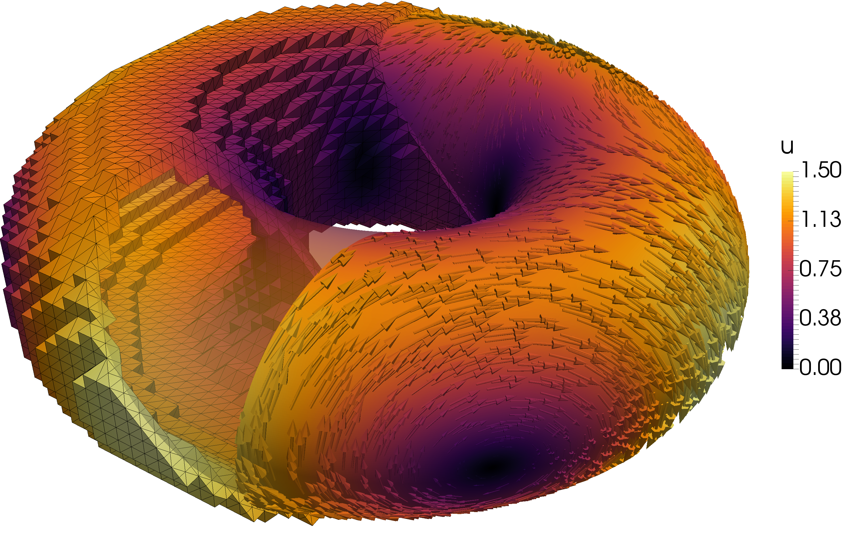
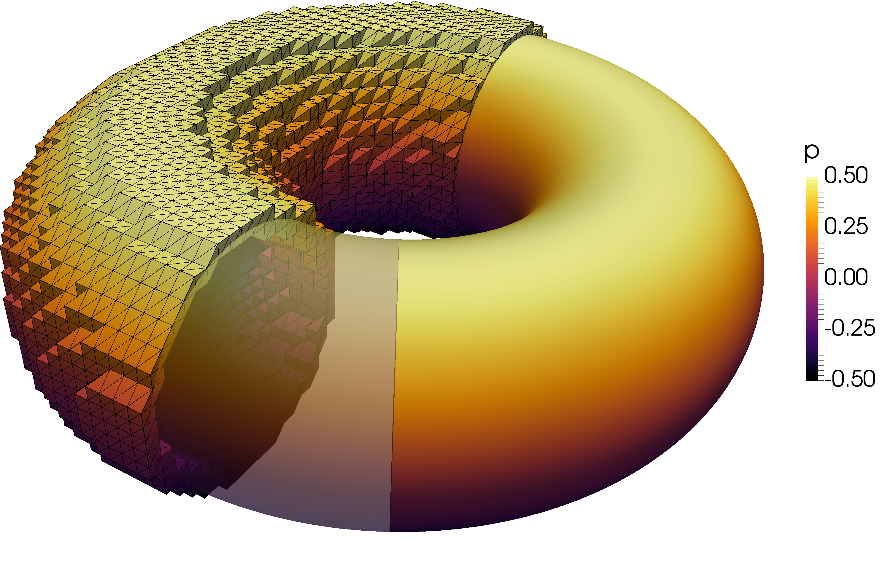
To study the combined effect of chosing various approximation orders $k_{u}$, $k_{p}$ and $k_{g}$ and stabilization forms $S_{h}^{i}$ on the overall approximation quality of the discrete solution, we conduct convergence experiments for 6 different scenarios. For each scenario, we compute the $L^{2}$ norm of the velocity error $e_{u}=u^{e}-u_{h}$ as well as the $H^{1}$ and $L^{2}$ norms of the pressure error $e_{p}=p^{e}-p_{h}$ which are displayed in Table 6.2. A short summary of the cases considered and the theoretically expected convergence rates are given Table 6.1. The computed EOC data in Table 6.2 clearly confirms the predicted convergence rates. In particular, we observe that increasing the pressure approximation to $k_{p}=2$ does only increase the convergence order for all considered error norms by one if both a high order approximation $k_{g}=2$ of ${\Gamma_{h}}$ and the higher-order consistent normal stabilization $S_{h}^{2}$ are used. Finally, the discrete solution components computed for $(k_{u},k_{p},k_{g})=(1,2,2)$ at the finest refinement level are visualized in Figure 6.1.

Case $k_{u}$ $k_{p}$ $k_{g}$ $S_{h}$ $\|e_{u}\|_{{\Gamma_{h}}}$ $\|e_{u}\|_{1,{\Gamma_{h}}}$ $\|e_{p}\|_{{\Gamma_{h}}}$
1 1 1 1 $S_{h}^{1}$ 1 1 2
2 1 1 1 $S_{h}^{2}$ 1 1 2
3 1 2 1 $S_{h}^{1}$ 1 1 2
4 1 2 1 $S_{h}^{2}$ 1 1 2
5 1 2 2 $S_{h}^{1}$ 1 1 2
6 1 2 2 $S_{h}^{2}$ 2 2 3
Table 6.1. Summary of the 6 cases considered in the convergence experiments and the corresponding theoretical convergence rates predicted by Theorem 5.3 and Theorem 5.4.
$k$ $\|u_{k}-u^{e}\|_{\Gamma_{h}}$ EOC $\|p_{k}-p^{e}\|_{1,\Gamma_{h}}$ EOC $\|p_{k}-p^{e}\|_{\Gamma_{h}}$ EOC
00 $9.71$ $\cdot 10^{-1}$ $1.10$ $\cdot 10^{0}$ $1.69$ $\cdot 10^{-1}$
$1$ $3.06$ $\cdot 10^{-1}$ $1.67$ $6.46$ $\cdot 10^{-1}$ $0.77$ $5.29$ $\cdot 10^{-2}$ $1.68$
$2$ $9.04$ $\cdot 10^{-2}$ $1.76$ $3.10$ $\cdot 10^{-1}$ $1.06$ $1.18$ $\cdot 10^{-2}$ $2.16$
$3$ $3.08$ $\cdot 10^{-2}$ $1.55$ $1.53$ $\cdot 10^{-1}$ $1.02$ $2.80$ $\cdot 10^{-3}$ $2.08$
$4$ $1.30$ $\cdot 10^{-2}$ $1.25$ $7.72$ $\cdot 10^{-2}$ $0.99$ $6.86$ $\cdot 10^{-4}$ $2.03$

(a) Case 1: $(k_{u},k_{p},k_{g})=(1,1,1)$ and full gradient stabilization $S_{h}=S_{h}^{1}$.
$k$ $\|u_{k}-u^{e}\|_{\Gamma_{h}}$ EOC $\|p_{k}-p^{e}\|_{1,\Gamma_{h}}$ EOC $\|p_{k}-p^{e}\|_{\Gamma_{h}}$ EOC
00 $4.70$ $\cdot 10^{-1}$ $1.28$ $\cdot 10^{0}$ $7.31$ $\cdot 10^{-2}$
$1$ $1.43$ $\cdot 10^{-1}$ $1.72$ $6.45$ $\cdot 10^{-1}$ $0.99$ $2.08$ $\cdot 10^{-2}$ $1.82$
$2$ $4.75$ $\cdot 10^{-2}$ $1.58$ $3.14$ $\cdot 10^{-1}$ $1.04$ $4.84$ $\cdot 10^{-3}$ $2.10$
$3$ $2.06$ $\cdot 10^{-2}$ $1.21$ $1.57$ $\cdot 10^{-1}$ $0.99$ $1.19$ $\cdot 10^{-3}$ $2.02$
$4$ $9.92$ $\cdot 10^{-3}$ $1.05$ $7.80$ $\cdot 10^{-2}$ $1.01$ $2.82$ $\cdot 10^{-4}$ $2.08$

(b) Case 2: $(k_{u},k_{p},k_{g})=(1,1,1)$ and normal gradient stabilization $S_{h}=S_{h}^{2}$.
$k$ $\|u_{k}-u^{e}\|_{\Gamma_{h}}$ EOC $\|p_{k}-p^{e}\|_{1,\Gamma_{h}}$ EOC $\|p_{k}-p^{e}\|_{\Gamma_{h}}$ EOC
00 $4.69$ $\cdot 10^{-1}$ $1.30$ $\cdot 10^{0}$ $7.42$ $\cdot 10^{-2}$
$1$ $1.43$ $\cdot 10^{-1}$ $1.72$ $6.46$ $\cdot 10^{-1}$ $1.01$ $2.08$ $\cdot 10^{-2}$ $1.83$
$2$ $4.75$ $\cdot 10^{-2}$ $1.58$ $3.14$ $\cdot 10^{-1}$ $1.04$ $4.85$ $\cdot 10^{-3}$ $2.10$
$3$ $2.06$ $\cdot 10^{-2}$ $1.21$ $1.57$ $\cdot 10^{-1}$ $0.99$ $1.19$ $\cdot 10^{-3}$ $2.02$
$4$ $9.92$ $\cdot 10^{-3}$ $1.05$ $7.80$ $\cdot 10^{-2}$ $1.01$ $2.82$ $\cdot 10^{-4}$ $2.08$

(c) Case 3: $(k_{u},k_{p},k_{g})=(1,2,1)$ and full gradient stabilization $S_{h}=S_{h}^{1}$.
$k$ $\|u_{k}-u^{e}\|_{\Gamma_{h}}$ EOC $\|p_{k}-p^{e}\|_{1,\Gamma_{h}}$ EOC $\|p_{k}-p^{e}\|_{\Gamma_{h}}$ EOC
00 $4.69$ $\cdot 10^{-1}$ $1.30$ $\cdot 10^{0}$ $7.42$ $\cdot 10^{-2}$
$1$ $1.43$ $\cdot 10^{-1}$ $1.72$ $6.46$ $\cdot 10^{-1}$ $1.01$ $2.08$ $\cdot 10^{-2}$ $1.83$
$2$ $4.75$ $\cdot 10^{-2}$ $1.58$ $3.14$ $\cdot 10^{-1}$ $1.04$ $4.85$ $\cdot 10^{-3}$ $2.10$
$3$ $2.06$ $\cdot 10^{-2}$ $1.21$ $1.57$ $\cdot 10^{-1}$ $0.99$ $1.19$ $\cdot 10^{-3}$ $2.02$

(d) Case 4: $(k_{u},k_{p},k_{g})=(1,2,1)$ and normal gradient stabilization $S_{h}=S_{h}^{2}$.
$k$ $\|u_{k}-u^{e}\|_{\Gamma_{h}}$ EOC $\|p_{k}-p^{e}\|_{1,\Gamma_{h}}$ EOC $\|p_{k}-p^{e}\|_{\Gamma_{h}}$ EOC
00 $3.61$ $\cdot 10^{0}$ $1.56$ $\cdot 10^{0}$ $3.58$ $\cdot 10^{-1}$
$1$ $2.47$ $\cdot 10^{0}$ $0.55$ $5.03$ $\cdot 10^{-1}$ $1.63$ $1.44$ $\cdot 10^{-1}$ $1.31$
$2$ $9.04$ $\cdot 10^{-1}$ $1.45$ $1.34$ $\cdot 10^{-1}$ $1.91$ $3.40$ $\cdot 10^{-2}$ $2.09$
$3$ $2.65$ $\cdot 10^{-1}$ $1.77$ $4.09$ $\cdot 10^{-2}$ $1.71$ $8.94$ $\cdot 10^{-3}$ $1.93$

(e) Case 5: $(k_{u},k_{p},k_{g})=(1,2,2)$ and full gradient stabilization $S_{h}=S_{h}^{1}$.
$k$ $\|u_{k}-u^{e}\|_{\Gamma_{h}}$ EOC $\|p_{k}-p^{e}\|_{1,\Gamma_{h}}$ EOC $\|p_{k}-p^{e}\|_{\Gamma_{h}}$ EOC
00 $1.55$ $\cdot 10^{0}$ $1.77$ $\cdot 10^{0}$ $1.71$ $\cdot 10^{-1}$
$1$ $2.94$ $\cdot 10^{-1}$ $2.40$ $4.12$ $\cdot 10^{-1}$ $2.10$ $1.72$ $\cdot 10^{-2}$ $3.31$
$2$ $4.73$ $\cdot 10^{-2}$ $2.63$ $9.63$ $\cdot 10^{-2}$ $2.10$ $1.49$ $\cdot 10^{-3}$ $3.53$
$3$ $8.64$ $\cdot 10^{-3}$ $2.45$ $2.33$ $\cdot 10^{-2}$ $2.05$ $1.15$ $\cdot 10^{-4}$ $3.69$

(f) Case 6: $(k_{u},k_{p},k_{g})=(1,2,2)$ and normal gradient stabilization $S_{h}=S_{h}^{2}$.
Table 6.2. Experimental order of convergence for the all 6 cases computed with a stabilization parameter $\tau=0.1$.

Acknowledgements

This research was supported in part by the Swedish Foundation for Strategic Research Grant No. AM13-0029, the Swedish Research Council Grants Nos. 2011-4992, 2013-4708, and Swedish strategic research programme eSSENCE.

References

  • Antonietti et al. [2016] P.F. Antonietti, C. Facciola, A. Russo, and M. Verani. Discontinuous galerkin approximation of flows in fractured porous media. Technical report, MOX, Dipartimento di Matematica Politecnico di Milano,, 2016.
  • Barreira et al. [2011] R Barreira, Charles M Elliott, and A Madzvamuse. The surface finite element method for pattern formation on evolving biological surfaces. Journal of mathematical biology, 63(6):1095–1119, 2011.
  • Burman et al. [2015a] E. Burman, S. Claus, P. Hansbo, M. G. Larson, and A. Massing. CutFEM: discretizing geometry and partial differential equations. Internat. J. Numer. Meth. Engrg, 104(7):472–501, November 2015a.
  • Burman et al. [2015b] E. Burman, P. Hansbo, and M. G. Larson. A stabilized cut finite element method for partial differential equations on surfaces: The Laplace–Beltrami operator. Comput. Methods Appl. Mech. Engrg., 285:188–207, 2015b.
  • Burman et al. [2015c] E. Burman, P. Hansbo, M. G. Larson, and S. Zahedi. Stabilized CutFEM for the convection problem on surfaces. arXiv preprint arXiv:1511.02340, pages 1–32, 2015c.
  • Burman et al. [2016] E. Burman, P. Hansbo, M. G. Larson, and A. Massing. Cut Finite Element Methods for Partial Differential Equations on Embedded Manifolds of Arbitrary Codimensions. ArXiv e-prints, October 2016.
  • Burman et al. [2016] E. Burman, P. Hansbo, M. G. Larson, and A. Massing. A cut discontinuous Galerkin method for the Laplace–Beltrami operator. IMA J. Numer. Anal., pages 1–32, 2016. doi: 10.1093/imanum/drv068.
  • Burman et al. [2016] E. Burman, P. Hansbo, M. G. Larson, A. Massing, and S. Zahedi. Full gradient stabilized cut finite element methods for surface partial differential equations. Comput. Methods Appl. Mech. Engrg., 310:278–296, October 2016. ISSN 0045-7825. doi: http://dx.doi.org/10.1016/j.cma.2016.06.033. URL http://www.sciencedirect.com/science/article/pii/S0045782516306703.
  • Burman et al. [2016] E. Burman, P. Hansbo, M.G. Larson, and S. Zahedi. Cut finite element methods for coupled bulk-surface problems. Numer. Math., 133:203–231, 2016.
  • Del Pra et al. [2015] Marco Del Pra, Alessio Fumagalli, and Anna Scotti. Well posedness of fully coupled fracture/bulk darcy flow with xfem. Technical Report 25, MOX, Department of Mathematics, Politecnico di Milano, 2015.
  • Demlow [2009] A. Demlow. Higher-order finite element methods and pointwise error estimates for elliptic problems on surfaces. SIAM Journal on Numerical Analysis, 47(2):805–827, 2009.
  • Dziuk [1988] G. Dziuk. Finite elements for the Beltrami operator on arbitrary surfaces. In Partial differential equations and calculus of variations, volume 1357 of Lecture Notes in Math., pages 142–155. Springer, Berlin, 1988.
  • Dziuk and Elliott [2013] G. Dziuk and C. M. Elliott. Finite element methods for surface PDEs. Acta Numer., 22:289–396, 2013.
  • Eilks and Elliott [2008] Carsten Eilks and Charles M Elliott. Numerical simulation of dealloying by surface dissolution via the evolving surface finite element method. Journal of Computational Physics, 227(23):9727–9741, 2008.
  • Elliott et al. [2012] Charles M Elliott, Björn Stinner, and Chandrasekhar Venkataraman. Modelling cell motility and chemotaxis with evolving surface finite elements. Journal of The Royal Society Interface, page rsif20120276, 2012.
  • Ern and Guermond [2004] A. Ern and J.-L. Guermond. Theory and Practice of Finite Elements, volume 159 of Appl. Math. Sci. Springer-Verlag, New York, 2004.
  • Evans and Gariepy [1992] L. C. Evans and R. F. Gariepy. Measure Theory and Fine Properties of Functions. Studies in Advanced Mathematics. CRC Press, Boca Raton, FL, 1992.
  • Ferroni et al. [2016] Alberto Ferroni, Luca Formaggia, and Alessio Fumagalli. Numerical analysis of Darcy problem on surfaces. ESAIM: Mathematical Modelling and Numerical Analysis, 50(6):1615–1630, 2016.
  • Flemisch et al. [2016] Bernd Flemisch, Alessio Fumagalli, and Anna Scotti. A review of the xfem-based approximation of flow in fractured porous media. In Advances in Discretization Methods: Discontinuities, Virtual Elements, Fictitious Domain Methods, volume 12, pages 47–76. Springer, 2016.
  • Fumagalli and Scotti [2013] A. Fumagalli and A. Scotti. A numerical method for two-phase flow in fractured porous media with non-matching grids. Adv. Water Resour., pages 1–11, April 2013. ISSN 03091708. doi: 10.1016/j.advwatres.2013.04.001.
  • Ganesan and Tobiska [2009] Sashikumaar Ganesan and Lutz Tobiska. A coupled arbitrary lagrangian–eulerian and lagrangian method for computation of free surface flows with insoluble surfactants. Journal of Computational Physics, 228(8):2859–2873, 2009.
  • Gilbarg and Trudinger [2001] D. Gilbarg and N. S. Trudinger. Elliptic Partial Differential Equations of Second Order. Classics in Mathematics. Springer-Verlag, Berlin, 2001.
  • Grande et al. [2016] J. Grande, C. Lehrenfeld, and A. Reusken. Analysis of a high order Trace Finite Element Method for PDEs on level set surfaces. ArXiv e-prints, November 2016.
  • Groß and Reusken [2011] S. Groß and A. Reusken. Numerical methods for two-phase incompressible flows, volume 40. Springer, 2011.
  • Groß et al. [2015] S. Groß, M. A. Olshanskii, and A. Reusken. A trace finite element method for a class of coupled bulk-interface transport problems. ESAIM: Math. Model. Numer. Anal., 49(5):1303–1330, Sept. 2015. doi: 10.1051/m2an/2015013.
  • Hansbo et al. [2003] A. Hansbo, P. Hansbo, and M. G. Larson. A finite element method on composite grids based on Nitsche’s method. ESAIM: Math. Model. Num. Anal., 37(3):495–514, 2003.
  • Hansbo et al. [2016] P. Hansbo, M. G. Larson, and S. Zahedi. A cut finite element method for coupled bulk-surface problems on time-dependent domains. Comput. Methods Appl. Mech. Engrg., 307:96–116, 2016.
  • Hansbo and Larson [2016] Peter Hansbo and Mats G. Larson. A stabilized finite element method for the darcy problem on surfaces. IMA Journal of Numerical Analysis, 2016. doi: 10.1093/imanum/drw041. URL http://imajna.oxfordjournals.org/content/early/2016/08/11/imanum.drw041.abstract.
  • Masud and Hughes [2002] Arif Masud and Thomas JR Hughes. A stabilized mixed finite element method for darcy flow. Computer Methods in Applied Mechanics and Engineering, 191(39):4341–4370, 2002.
  • Novak et al. [2007] Igor L Novak, Fei Gao, Yung-Sze Choi, Diana Resasco, James C Schaff, and Boris M Slepchenko. Diffusion on a curved surface coupled to diffusion in the volume: Application to cell biology. Journal of computational physics, 226(2):1271–1290, 2007.
  • Olshanskii and Reusken [2014] M. A. Olshanskii and A. Reusken. Error analysis of a space-time finite element method for solving PDEs on evolving surfaces. SIAM J. Numer. Anal., 52(4):2092–2120, 2014.
  • Olshanskii et al. [2009] M. A. Olshanskii, A. Reusken, and J. Grande. A finite element method for elliptic equations on surfaces. SIAM J. Numer. Anal., 47(5):3339–3358, 2009.
  • Olshanskii et al. [2014a] M. A. Olshanskii, A. Reusken, and X. Xu. A stabilized finite element method for advection–diffusion equations on surfaces. IMA J. Numer. Anal., 34(2):732–758, 2014a.
  • Olshanskii et al. [2014b] M. A. Olshanskii, A. Reusken, and X. Xu. An Eulerian space-time finite element method for diffusion problems on evolving surfaces. SIAM J. Numer. Anal., 52(3):1354–1377, 2014b.
  • Reusken [2014] A. Reusken. Analysis of trace finite element methods for surface partial differential equations. IMA J. Numer. Anal., 35:1568–1590, 2014.