Generalized Riemann sums

Abstract.

The primary aim of this chapter is, commemorating the 150th anniversary of Riemann’s death, to explain how the idea of Riemann sum is linked to other branches of mathematics. The materials I treat are more or less classical and elementary, thus available to the “common mathematician in the streets.” However one may still see here interesting inter-connection and cohesiveness in mathematics.

1. Introduction

On Gauss’s recommendation, Bernhard Riemann presented the paper Über die Darstellbarkeit einer Function durch eine trigonometrische Reihe to the Council of Göttingen University as his Habilitationsschrift at the first stage in December of 1853. As the title clearly suggests, the aim of his essay was to lay the foundation for the theory of trigonometric series (Fourier series in today’s term).

The record of previous work by other mathematicians, to which Riemann devoted three sections of the essay, tells us that the Fourier series had been used to represent general solutions of the wave equation and the heat equation without any convincing proof of convergence. For instance, Fourier claimed, in his study of the heat equation (1807, 1822), that if we put

(1.1) $$a_{n}=\frac{1}{\pi}\int_{-\pi}^{\pi}f(x)\sin nx~{}\!dx,\quad b_{n}=\frac{1}{\pi}\int_{-\pi}^{\pi}f(x)\cos nx~{}\!dx,$$

then

(1.2) $$f(x)=\frac{1}{2}b_{0}+(a_{1}\sin x+b_{1}\cos x)+(a_{2}\sin 2x+b_{2}\cos 2x)+\cdots$$

without any restrictions on the function $f(x)$. But this is not true in general as is well known. What is worse (though, needless to say, the significance of his paper as a historical document cannot be denied) is his claim that the integral of an “arbitrary” function is meaningful as the area under/above the associated graph.

L. Dirichlet, a predecessor of Riemann, was the first who gave a solid proof for convergence in a special case. Actually he proved that the right-hand side of (1.2) converges to $\displaystyle\frac{1}{2}\big{(}f(x+0)+f(x-0)\big{)}$ for a class of functions including piecewise monotone continuous functions (1829). Stimulated by Dirichlet’s study, Riemann made considerable progress on the convergence problem. In the course of his discussion, he gave a precise notion of integrability of a function, and then obtained a condition for an integrable function to be representable by a Fourier series. Furthermore he proved that the Fourier coefficients for any integrable function $a_{n},b_{n}$ converge to zero as $n\to\infty$. This theorem, which was generalized by Lebesgue later to a broader class of functions, is to be called the Riemann-Lebesgue theorem, and is of importance in Fourier analysis and asymptotic analysis.

What plays a significant role in Riemann’s definition of integrals is the notion of Riemann sum, which, if we use his notation (Fig. ​1), is expressed as

$$S=\delta_{1}f(a+\epsilon_{1}\delta_{1})+\delta_{2}f(x_{1}+\epsilon_{2}\delta_{2})+\delta_{3}f(x_{3}+\epsilon_{3}\delta_{3})+\cdots+\delta_{n}f(x_{n-1}+\epsilon_{n}\delta_{n}).$$

Here $f(x)$ is a function on the closed interval $[a,b]$, $a=x_{0}<x_{1}<x_{2}<\cdots<x_{n-1}<x_{n}=b$, and $\delta_{i}=x_{i}-x_{i-1}$ ($i=1,2,\ldots,n$). If $S$ converges to $A$ as $\max_{i}\delta_{i}$ goes to $0$ whatever $\epsilon_{i}$ with $0<\epsilon_{i}<1$ ($i=1,\ldots,n$) are chosen (thus $x_{k-1}+\epsilon_{k}\delta_{k}\in[x_{k-1},x_{k}]$), then the value $A$ is written as $\displaystyle\int_{a}^{b}f(x)dx$, and $f(x)$ is called Riemann integrable. For example, every continuous function is Riemann integrable as we learn in calculus.

Compared with Riemann’s other supereminent works, his essay looks unglamorous. Indeed, from today’s view, his formulation of integrability is no more than routine. But the harbinger must push forward through the total dark without any definite idea of the direction. All he needs is a torch of intelligence.

The primary aim of this chapter is not to present the subsequent development after Riemann’s work on integrals such as the contribution by C. Jordan (1892), G. Peano (1887), H. L. Lebesgue (1892), T. J. Stieltjes (1894), and K. Ito (1942), but to explain how the idea of Riemann sum is linked to other branches of mathematics; for instance, some counting problems in elementary number theory and the theory of quasicrystals, the former having a long history and the latter being an active field still in a state of flux.

I am very grateful to Xueping Guang for drawing attention to Ref. ​[11] which handles some notions closely related to the ones in the present chapter.

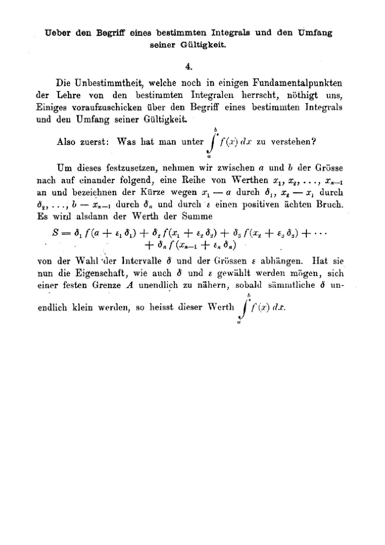
Figure 1. Riemann’s paper

2. Generalized Riemann sums

The notion of Riemann sum is immediately generalized to functions of several variables as follows.

Let $\Delta=\{D_{\alpha}\}_{\alpha\in A}$ be a partition of $\mathbb{R}^{d}$ by a countable family of bounded domains $D_{\alpha}$ with piecewise smooth boundaries satisfying

(i)  ${\rm mesh}(\Delta):=\displaystyle\sup_{\alpha\in A}d(D_{\alpha})<\infty$, where $d(D_{\alpha})$ is the diameter of $D_{\alpha}$,

(ii)  there are only finitely many $\alpha$ such that $K\cap D_{\alpha}\neq\emptyset$ for any compact set $K\subset\mathbb{R}^{d}$.

We select a point ${\boldsymbol{\xi}}_{\alpha}$ from each $D_{\alpha}$, and put $\Gamma=\{\boldsymbol{\xi}_{\alpha}|~{}\alpha\in A\}$. The Riemann sum $\sigma(f,\Delta,\Gamma)$ for a function $f$ on $\mathbb{R}^{d}$ with compact support is defined by

$$\sigma(f,\Delta,\Gamma)=\sum_{\alpha\in A}f({\boldsymbol{\xi}}_{\alpha}){\rm vol}(D_{\alpha}),$$

where ${\rm vol}(D_{\alpha})$ is the volume of $D_{\alpha}$. Note that $f({\boldsymbol{\xi}}_{\alpha})=0$ for all but finitely many $\alpha$ because of Property (ii).

If the limit

$$\lim_{{\rm mesh}(\Delta)\to 0}\sigma(f,\Delta,\Gamma)$$

exists, independently of the specific sequence of partitions and the choice of $\{{\boldsymbol{\xi}}_{\alpha}\}$, then $f$ is said to be Riemann integrable, and this limit is called the ($d$-tuple) Riemann integral of $f$, which we denote by $\displaystyle\int_{\mathbb{R}^{d}}f({\bf x})d{\bf x}$.

In particular, if we take the sequence of partitions given by$\Delta_{\epsilon}=\{\epsilon D_{\alpha}|~{}\alpha\in A\}$ ($\epsilon>0$), then, for every Riemann integrable function $f$, we have

(2.1) $$\lim_{\epsilon\to+0}\sum_{\alpha\in A}\epsilon^{d}f(\epsilon{\boldsymbol{\xi}}_{\alpha}){\rm vol}(D_{\alpha})=\int_{\mathbb{R}^{d}}f({\bf x})d{\bf x},$$

where we should note that ${\rm vol}(\epsilon D_{\alpha})=\epsilon^{d}{\rm vol}(D_{\alpha})$.

Now we look at Eq. ​2.1 from a different angle. We think that $\omega(\boldsymbol{\xi}_{\alpha}):={\rm vol}(D_{\alpha})$ is a weight of the point $\boldsymbol{\xi}_{\alpha}$, and that Eq. ​2.1 is telling how the weighted discrete set $(\Gamma,\omega)$ is distributed in $\mathbb{R}^{d}$; more specifically we may consider that Eq. ​2.1 implies uniformity, in a weak sense, of $(\Gamma,\omega)$ in $\mathbb{R}^{d}$. This view motivates us to propose the following definition.

In general, a weighted discrete subset in $\mathbb{R}^{d}$ is a discrete set $\Gamma\subset\mathbb{R}^{d}$ with a function $\omega:\Gamma\rightarrow\mathbb{C}\backslash\{0\}$. Given a compactly supported function $f$ on $\mathbb{R}^{d}$, define the (generalized) Riemann sum associated with $(\Gamma,\omega)$ by setting

$$\sigma(f,\Gamma,\omega)=\sum_{{\bf z}\in\Gamma}f({\bf z})\omega({\bf z}).$$

In addition, we say that $(\Gamma,\omega)$ has constant density $c(\Gamma,\omega)\neq 0$ (Marklof and Strömbergsson [10]) if

(2.2) $$\lim_{\epsilon\to+0}\sigma(f^{\epsilon},\Gamma,\omega)\Big{(}=\lim_{\epsilon\to+0}\sum_{z\in\Gamma}\epsilon^{d}f(\epsilon z)\omega(z)\Big{)}=c(\Gamma,\omega)\int_{\mathbb{R}^{d}}f({\bf x})d{\bf x}$$

holds for any bounded Riemann integrable function $f$ on $\mathbb{R}^{d}$ with compact support, where $\displaystyle f^{\epsilon}(x)=\epsilon^{d}f(\epsilon x)$; thus the weighted discrete set associated with a partition $\{D_{\alpha}\}$ and $\{\boldsymbol{\xi}_{\alpha}\}$ has constant density $1$. In the case $\omega\equiv 1$, we write $\sigma(f,\Gamma)$ for $\sigma(f,\Gamma,\omega)$, and $c(\Gamma)$ for $c(\Gamma,\omega)$ when $\Gamma=(\Gamma,\omega)$ has constant density.

In connection with the notion of constant density, it is perhaps worth recalling the definition of a Delone set, a qualitative concept of “uniformity”. A discrete set $\Gamma$ is called a Delone set if it satisfies the following two conditions (Delone [4]).

(1) There exists $R>0$ such that every ball $B_{R}(x)$ (of radius $R$ whose center is $x$) has a nonempty intersection with $\Gamma$, i.e., $\Gamma$ is relatively dense;

(2) there exists $r>0$ such that each ball $B_{r}(x)$ contains at most one element of $\Gamma$, i.e., $\Gamma$ is uniformly discrete.

The following proposition states a relation between Delone sets and Riemann sums.

Proposition 2.1.

Let $\Gamma$ be a Delone set. Then there exist positive constants $c_{1},c_{2}$ such that

$$c_{1}\int_{\mathbb{R}^{d}}f({\bf x})d{\bf x}\leq\varliminf_{\epsilon\to+0}\sigma(f^{\epsilon},\Gamma)\leq\varlimsup_{\epsilon\to+0}\sigma(f^{\epsilon},\Gamma)\leq c_{2}\int_{\mathbb{R}^{d}}f({\bf x})d{\bf x}$$

for every nonnegative-valued function $f$.

Proof In view of the Delone property, one can find two partitions $\{D_{\alpha}\}$ and $\{D^{\prime}_{\beta}\}$ consisting of rectangular parallelotopes satisfying

(i)  Every $D_{\alpha}$ has the same size, and contains at least one element of $\Gamma$;

(ii)  every $D^{\prime}_{\beta}$ has the same size, and contains at most one element of $\Gamma$.

Put $c_{1}={\rm vol}(D_{\alpha})^{-1}$ and $c_{2}={\rm vol}(D^{\prime}_{\beta})^{-1}$. We take a subset $\Gamma_{1}$ of $\Gamma$ such that every $D_{\alpha}$ contains just one element of $\Gamma_{1}$, and also take $\Gamma_{2}\supset\Gamma$ such that every $D^{\prime}_{\beta}$ contains just one element of $\Gamma_{2}$. We then have $\sigma(f^{\epsilon},\Gamma_{1})\leq\sigma(f^{\epsilon},\Gamma)\leq\sigma(f^{\epsilon},\Gamma_{2})$. Therefore using Eq. ​2.1, we have

$$c_{1}\int_{\mathbb{R}^{d}}f({\bf x})d{\bf x}=\lim_{\epsilon\to+0}\sigma(f^{\epsilon},\Gamma_{1})\leq\varliminf_{\epsilon\to+0}\sigma(f^{\epsilon},\Gamma)$$

$$\qquad\leq\varlimsup_{\epsilon\to+0}\sigma(f^{\epsilon},\Gamma)\leq\lim_{\epsilon\to+0}\sigma(f^{\epsilon},\Gamma_{2})=c_{2}\int_{\mathbb{R}^{d}}f({\bf x})d{\bf x},$$

where we should note that $\sigma_{\epsilon}(f,\Gamma_{1})$ and $\sigma_{\epsilon}(f,\Gamma_{2})$ are ordinary Riemann sums. $\Box$

One might ask “what is the significance of the notions of generalized Riemann sum and constant density?” Admittedly these notions are not so much profound (one can find more or less the same concepts in plural references). It may be, however, of great interest to focus our attention on the constant $c(\Gamma,\omega)$. In the subsequent sections, we shall give two “arithmetical” examples for which the constant $c(\Gamma)$ is explicitly computed.

3. Classical example 1

Let $\mathbb{Z}_{\rm prim}^{d}$ $~{}(d\geq 2)$ be the set of primitive lattice points in the $d$-dimensional standard lattice $\mathbb{Z}^{d}$, i.e., the set of lattice points visible from the origin (note that $\mathbb{Z}_{\rm prim}^{2}$ is the set of $(x,y)\in\mathbb{Z}^{2}$ such that $(|x|,|y|)$ is a coprime pair of positive integers, together with $(\pm 1,0)$ and $(0,\pm 1)$).

Theorem 3.1.

$\mathbb{Z}_{\rm prim}^{d}$ has constant density $\zeta(d)^{-1}$; that is,

$$\lim_{\epsilon\to+0}\sum_{{\bf z}\in\mathbb{Z}_{\rm prim}^{d}}\epsilon^{d}f(\epsilon{\bf z})=\zeta(d)^{-1}\int_{\mathbb{R}^{d}}f({\bf x})d{\bf x}.$$

Here $\displaystyle\zeta(s)=\sum_{n=1}^{\infty}n^{-s}$ is the zeta function.

The proof, which is more or less known as a sort of folklore, will be indicated in Sect. ​5.

Noting that $\zeta(2)=\pi^{2}/6$ and applying this theorem to the indicator function $f$ for the square $\{(x,y)|~{}0\leq x,y\leq 1\}$, we obtain the following well-known statement.

Corollary 3.1.

The probability that two randomly chosen positive integers are coprime is $6/\pi^{2}$. More precisely

$$\lim_{N\to\infty}\frac{1}{N^{2}}\big{|}\big{\{}(a,b)\in\mathbb{N}\times\mathbb{N}|~{}{\rm gcd}(a,b)=1,~{}a,b\leq N\big{\}}\big{|}=\frac{6}{\pi^{2}},$$

where ${\rm gcd}(a,b)$ stands for the greatest common divisor of $a,b$.

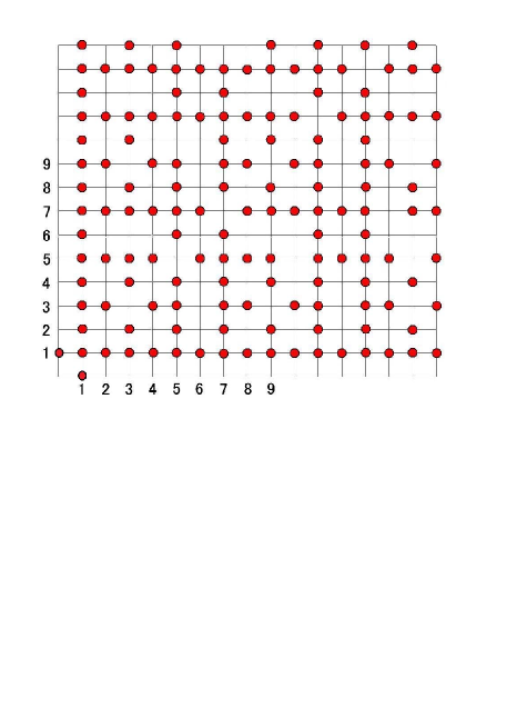
Figure 2. Coprime pairs

Remark 3.1.

(1)  Gauss’s Mathematisches Tagebuch (Mathematical Diary), a record of the mathematical discoveries of C. F. Gauss from 1796 to 1814, contains 146 entries, most of which consist of brief and somewhat cryptical statements. Some of the statements which he never published were independently discovered and published by others often many years later.

The entry relevant to Corollary 3.1 is the 31st dated 1796 September 6:

“Numero fractionum inaequalium quorum denomonatores certum limitem non superant ad numerum fractionum omnium quarum num[eratores] aut denom[inatores] sint diversi infra limitem in infinito ut $6:\pi\pi$”

This vague statement about counting (irreducible) fractions was formulated in an appropriate way afterwards and proved rigorously by Dirichlet (1849) and Ernesto Cesàro (1881). As a matter of fact, because of its vagueness, there are several ways to interpret what Gauss was going to convey.

(2)  In connection with Theorem 3.1, it is perhaps worthwhile to make reference to the Siegel mean value theorem ([15]).

Let $g\in\mathrm{SL}_{d}(\mathbb{R})$. For a bounded Riemann integrable function $f$ on $\mathbb{R}^{d}$ with compact support, we consider

$$\varPhi(g)=\sum_{{\bf z}\in\mathbb{Z}^{d}\backslash\{{\bf 0}\}}f(g{\bf z}),\quad\Psi(g)=\sum_{{\bf z}\in\mathbb{Z}_{{\rm prim}}^{d}}f(g{\bf z}).$$

Both functions $\varPhi$ and $\Psi$ are $\mathrm{SL}_{d}(\mathbb{Z})$-invariant with respect to the right action of $\mathrm{SL}_{d}(\mathbb{Z})$ on $\mathrm{SL}_{d}(\mathbb{R})$, so that these are identified with functions on the coset space $\mathrm{SL}_{d}(\mathbb{R})/\mathrm{SL}_{d}(\mathbb{Z})$. Recall that $\mathrm{SL}_{d}(\mathbb{R})/\mathrm{SL}_{d}(\mathbb{Z})$ has finite volume with respect to the measure $dg$ induced from the Haar measure on $\mathrm{SL}_{d}(\mathbb{R})$. We assume $\displaystyle\int_{\mathrm{SL}_{d}(\mathbb{R})/\mathrm{SL}_{d}(\mathbb{Z})}1~{}dg=1$. Then the Siegel theorem asserts

$$\int_{\mathrm{SL}_{d}(\mathbb{R})/\mathrm{SL}_{d}(\mathbb{Z})}\Big{(}\sum_{{\bf z}\in\mathbb{Z}^{d}\backslash\{{\bf 0}\}}f(g{\bf z})\Big{)}dg=\int_{\mathbb{R}^{d}}f({\bf x})d{\bf x},$$

$$\int_{\mathrm{SL}_{d}(\mathbb{R})/\mathrm{SL}_{d}(\mathbb{Z})}\Big{(}\sum_{{\bf z}\in\mathbb{Z}_{{\rm prim}}^{d}}f(g{\bf z})\Big{)}dg=\zeta(d)^{-1}\int_{\mathbb{R}^{d}}f({\bf x})d{\bf x}.$$

$\Box$

4. Classical example 2

A Pythagorean triple, the name stemming from the Pythagorean theorem for right triangles, is a triple of positive integers $(\ell,m,n)$ satisfying the equation $\ell^{2}+m^{2}=n^{2}$. Since $(\ell/n)^{2}+(m/n)^{2}=1$, a Pythagorean triple yields a rational point $(\ell/n,m/n)$ on the unit circle $S^{1}=\{(x,y)|~{}x^{2}+y^{2}=1\}$. Conversely any rational point on $S^{1}$ is derived from a Pythagorean triple. Furthermore the well-known parameterization of $S^{1}$ given by $x=(1-t^{2})/(1+t^{2})$, $y=2t/(1+t^{2})$ tells us that the set of rational points $S^{1}(\mathbb{Q})=S^{1}\cap\mathbb{Q}^{2}$ is dense in $S^{1}$ (we shall see later how rational points are distributed from a quantitative viewpoint).

A Pythagorean triple $(x,y,z)$ is called primitive if $x,y,z$ are pairwise coprime. “Primitive” is so named because any Pythagorean triple is generated trivially from the primitive one, i.e., if $(x,y,z)$ is Pythagorean, there are a positive integer $\ell$ and a primitive $(x_{0},y_{0},z_{0})$ such that $(x,y,z)=(\ell x_{0},\ell y_{0},\ell z_{0})$.

The way to produce primitive Pythagorean triples (PPTs) is described as follows: If $(x,y,z)$ is a PPT, then there exist positive integers $m,n$ such that

(i)  $m>n$,

(ii)  $m$ and $n$ are coprime,

(iii)  $m$ and $n$ have different parity,

(iv) $~{}(x,y,z)=(m^{2}-n^{2},2mn,m^{2}+n^{2})$ or $(x,y,z)$ $=$ $(2mn,m^{2}-n^{2},m^{2}+n^{2})$.

Conversely, if $m$ and $n$ satisfy (i), (ii), (iii), then $(m^{2}-n^{2},2mn,m^{2}+n^{2})$ and $(2mn,m^{2}-n^{2},m^{2}+n^{2})$ are PPTs.

In the table below, due to M. Somos [16], of PPTs $(x,y,z)$ enumerated in ascending order with respect to $z$, the triple $(x_{N},y_{N},z_{N})$ is the $N$-th PPT (we do not discriminate between $(x,y,z)$ and $(y,x,z)$).

$N$	$x_{N}$	$y_{N}$	$z_{N}$
1	3	4	5
2	5	12	13
3	15	8	17
4	7	24	25
5	21	20	29
6	35	12	37
7	9	40	41
8	45	28	53
9	11	60	61
10	63	16	65

$N$	$x_{N}$	$y_{N}$	$z_{N}$
11	33	56	65
12	55	48	73
13	77	36	85
14	13	84	85
15	39	80	89
16	65	72	97
17	99	20	101
18	91	60	109
19	15	112	113
20	117	44	125

$\cdots$ $N$ $x_{N}$ $y_{N}$ $z_{N}$ 1491 4389 8300 9389 1492 411 9380 9389 1493 685 9372 9397 1494 959 9360 9409 1495 9405 388 9413 1496 5371 7740 9421 1497 9393 776 9425 1498 7503 5704 9425 1499 6063 7216 9425 1500 1233 9344 9425

What we have interest in is the asymptotic behavior of $z_{N}$ as $N$ goes to infinity. The numerical observation tells us that the sequence $\{z_{N}\}$ almost linearly increases as $N$ increases. Indeed $z_{100}/100=6.29,~{}z_{1000}/1000=6,277,z_{1500}/1500=6.28333\cdots$, which convinces us that $\displaystyle\lim_{N\to\infty}z_{N}/N$ exists (though the speed of convergence is very slow), and the limit is expected to be equal to $2\pi=6.2831853\cdots$. This is actually true as shown by D. N. Lehmer [9] in 1900, though his proof is by no means easy.

We shall prove Lehmer’s theorem by counting coprime pairs $(m,n)$ satisfying the condition that $m-n$ is odd. A key of our proof is the following theorem.

Theorem 4.1.

$\mathbb{Z}_{\rm prim}^{2,*}=\{(m.n)\in\mathbb{Z}_{\rm prim}^{2}|~{}m-n~{}\text{is odd}\}~{}(=\{(m.n)\in\mathbb{Z}_{\rm prim}^{2}|~{}m-n\equiv 1~{}\text{(\rm mod~{}2})\})$ has constant density $4/\pi^{2}$; namely

(4.1) $$\lim_{\epsilon\to+0}\sum_{{\bf z}\in\mathbb{Z}_{\rm prim}^{2,*}}\epsilon^{2}f(\epsilon{\bf z})=\frac{2}{3}\zeta(2)^{-1}\int_{\mathbb{R}^{2}}f({\bf x})d{\bf x}=\frac{4}{\pi^{2}}\int_{\mathbb{R}^{2}}f({\bf x})d{\bf x}.$$

We postpone the proof to Sect. ​5, and apply this theorem to the indicator function $f$ for the set $\{(x,y)\in\mathbb{R}^{2}|~{}\!x\geq y,~{}x^{2}+y^{2}\leq 1\}$. Since

$$\sum_{{\bf z}\in\mathbb{Z}_{\rm prim}^{2,*}}\epsilon^{2}f(\epsilon{\bf z})=\epsilon^{2}\big{|}\big{\{}(m,n)\in\mathbb{N}^{2}|~{}{\rm gcd}(m,n)=1,~{}m>n,$$

$$\qquad\qquad\qquad\qquad m^{2}+n^{2}\leq\epsilon^{-2},~{}m-n~{}\text{is odd}\big{\}}\big{|},$$

we obtain

(4.2) $$\lim_{N\to\infty}\frac{1}{N}\big{|}\big{\{}(m,n)\in\mathbb{N}^{2}|~{}{\rm gcd}(m,n)=1,~{}m>n,~{}m^{2}+n^{2}\leq N,$$

$$\qquad\qquad\qquad m-n~{}\text{is odd}\big{\}}\big{|}=\frac{2}{3}\cdot\frac{6}{\pi^{2}}\cdot\frac{\pi}{8}=\frac{1}{2\pi}.$$

Note that $\big{|}\big{\{}(m,n)\in\mathbb{N}^{2}|~{}{\rm gcd}(m,n)=1,~{}m>n,~{}m^{2}+n^{2}\leq N,~{}m-n~{}\text{is odd}\big{\}}\big{|}$ coincides with the number of PPT $(x,y,z)$ with $z\leq N$. This observation leads us to

Corollary 4.1.

(Lehmer) $\displaystyle\lim_{N\to\infty}\frac{z_{N}}{N}=2\pi$.

Remark 4.1.

Fermat’s theorem on sums of two squares, together with his little theorem and the formula $(a^{2}+b^{2})(c^{2}+d^{2})=(ac\pm bd)^{2}+(ad\mp bc)^{2}$, yields the following complete characterization of PPTs which is substantially equivalent to the result stated in the letter from Fermat to Mersenne dated 25 December 1640 (cf. ​Weil [20]).

An odd number $z$ is written as $m^{2}+n^{2}$ by using two coprime positive integers $m,n$ (thus automatically having different parity) if and only if every prime divisor of $z$ is of the form $4k+1$. In other words, the set $\{z_{N}\}$ coincides with the set of odd numbers whose prime divisors are of the form $4k+1$. Moreover, if we denote by $\nu(z)$ the number of distinct prime divisors of $z$, then $z=z_{N}$ in the list is repeated $2^{\nu(z)-1}$ times. $\Box$

Theorem 4.1 can be used to establish

Corollary 4.2.

For a rational point $(p,q)\in S^{1}(\mathbb{Q})(=S^{1}\cap\mathbb{Q}^{2})$, define the height $h(p,q)$ to be the minimal positive integer $h$ such that $(hp,hq)\in\mathbb{Z}^{2}$. Then for any arc $A$ in $S^{1}$, we have

$$\big{|}\big{\{}(p,q)\in A\cap\mathbb{Q}^{2}|~{}h(p,q)\leq h\big{\}}\big{|}\sim\frac{2\cdot{\rm length}(A)}{\pi^{2}}h\quad(h\to\infty),$$

and hence rational points are equidistributed on the unit circle in the sense that

$$\lim_{h\to\infty}\frac{\big{|}\big{\{}(p,q)\in A\cap\mathbb{Q}^{2}|~{}h(p,q)\leq h\big{\}}\big{|}}{\big{|}\big{\{}(p,q)\in S^{1}\cap\mathbb{Q}^{2}|~{}h(p,q)\leq h\}\big{|}}=\frac{{\rm length}(A)}{2\pi}.$$

In his paper [5], W. Duke suggested that this corollary can be proved by using tools from the theory of $L$-functions combined with Weyl’s famous criterion for equidistribution on the circle ([21]). Our proof below relies on a generalization of Eq. ​4.2.

Given $\alpha,\beta$ with $0\leq\alpha<\beta\leq 1$, we put

$$P(N;\alpha,\beta)=\big{\{}(m,n)\in\mathbb{N}\times\mathbb{N}|~{}{\rm gcd}(m,n)=1,\alpha\leq n/m\leq\beta,$$

$$\qquad\qquad m-n~{}\text{is odd},~{}m^{2}+n^{2}\leq N\big{\}}.$$

Namely we count coprime pairs $(m,n)$ with odd $m-n$ in the circular sector

$$\{(x,y)\in\mathbb{R}^{2}|~{}x,y>0,~{}\alpha x\leq y\leq\beta x,~{}x^{2}+y^{2}\leq N\}.$$

Since the area of the region $\{(x,y)\in\mathbb{R}^{2}|~{}x,y>0,~{}\alpha x\leq y\leq\beta x,~{}x^{2}+y^{2}\leq 1\}$ is $\displaystyle\frac{1}{2}\arctan\frac{\beta-\alpha}{1+\alpha\beta}$, applying again Eq. ​4.1 to the indicator function for this region, we obtain

$$\lim_{N\to\infty}\frac{1}{N}\big{|}P(N;\alpha,\beta)\big{|}=\frac{2}{\pi^{2}}\arctan\frac{\beta-\alpha}{1+\alpha\beta}.$$

Now we sort points $(p,q)\neq(\pm 1,0),(0,$ $\pm 1)$ in $S^{1}(\mathbb{Q})$ by 4 quadrants containing $(p,q)$, and also by parity of $x$ when we write $|p|=x/z$, $|q|=y/z$ with a PPT $(x,y,z)$. Here we should notice that $h(p,q)=z=m^{2}+n^{2}$. Thus counting rational points with the height function $h(p,q)$ reduces to counting PPTs.

Put

$$S_{\mathbb{Q}}^{1}({\rm odd})=\big{\{}(p,q)\in S^{1}(\mathbb{Q})|~{}\text{$x$ is odd}\big{\}},$$

$$S_{\mathbb{Q}}^{1}({\rm even})=\big{\{}(p,q)\in S^{1}(\mathbb{Q})|~{}\text{$x$ is even}\big{\}}.$$

Then

$$S^{1}(\mathbb{Q})=S_{\mathbb{Q}}^{1}({\rm odd})\cup S_{\mathbb{Q}}^{1}({\rm even})\cup\big{\{}(\pm 1,0),(0,\pm 1)\big{\}}\quad(\text{disjoint}).$$

Note that the correspondence $(p,q)\mapsto(q,p)$ interchanges $S_{\mathbb{Q}}^{1}({\rm odd})$ and $S_{\mathbb{Q}}^{1}({\rm even})$. Therefore, in order to complete the proof, it is enough to show that

$$\big{|}\big{\{}(p,q)\in S_{\mathbb{Q}}^{1}({\rm odd})|~{}\theta_{1}\leq\theta(p,q)<\theta_{2},~{}h(p,q)\leq h\big{\}}\big{|}$$

$$\sim \frac{1}{\pi^{2}}(\theta_{2}-\theta_{1})h\quad(h\to\infty),$$

where $(p,q)=\big{(}\cos\theta(p,q),\sin\theta(p,q)\big{)}$. Without loss of generality, one may assume $0\leq\theta_{1}<\theta_{2}\leq\pi/2$. Since

$$\tan\theta(p,q)=\frac{q}{p}=\frac{2mn}{m^{2}-n^{2}}=\frac{2\displaystyle\frac{n}{m}}{1-\Big{(}\displaystyle\frac{n}{m}\Big{)}^{2}},$$

if we define $\Theta(m,n)\in[0,\pi/2)$ by $\tan\Theta(m,n)=n/m$, then $\tan\theta(p,q)=\tan 2\Theta(m,n)$, and hence $\theta(p,q)=2\Theta(m,n)$. Therefore

$$\big{|}\big{\{}(p,q)\in S_{\mathbb{Q}}^{1}({\rm odd})|~{}\theta_{1}\leq\theta(g)<\theta_{2},~{}h(p,q)\leq h\big{\}}\big{|}$$

$$= \big{|}P(h;\arctan\theta_{1}/2,\arctan\theta_{2}/2)\big{|}$$

$$\sim \frac{1}{\pi^{2}}(\theta_{2}-\theta_{1})h,$$

as required.

Remark 4.2.

Interestingly, $S^{1}(\mathbb{Q})$ (and hence Pythagorean triples) has something to do with crystallography. Indeed $S^{1}(\mathbb{Q})$ with the natural group operation is an example of coincidence symmetry groups that show up in the theory of crystalline interfaces and grain boundaries in polycrystalline materials (Ranganathan [12], Zeiner [23]). This theory is concerned with partial coincidence of lattice points in two identical crystal lattices. See [18] for the details, and also [17] for the mathematical theory of crystal structures. $\Box$

5. The Inclusion-Exclusion Principle

The proof that the discrete sets $\mathbb{Z}^{d}_{\rm prim}$ and $\mathbb{Z}^{2,*}_{\rm prim}$ have constant density relies on the identities derived from the so-called Inclusion-Exclusion Principle (IEP), which is a generalization of the obvious equality $|A\cup B|=|A|+|B|-|A\cap B|$ for two finite sets $A,B$. Despite its simplicity, the IEP is a powerful tool to approach general counting problems involving aggregation of things that are not mutually exclusive (Comtet [1]).

To state the IEP in full generality, we consider a family $\{A_{h}\}_{h=1}^{\infty}$ of subsets of $X$ where $X$ and $A_{h}$ are not necessarily finite. Let $f$ be a real-valued function with finite support defined on $X$. We assume that there exists $N$ such that if $h>N$, then $A_{h}\cap{\rm supp}~{}\!f=\emptyset$, i.e. $f(x)=0$ for $x\in A_{h}$. In the following theorem, the symbol $A^{c}$ means the complement of a subset $A$ in $X$.

Theorem 5.1.

(Inclusion-Exclusion Principle)

$$\sum_{x\in\bigcap_{h=1}^{\infty}A_{h}^{c}}f(x) = \sum_{k=0}^{\infty}(-1)^{k}\sum_{h_{1}<\cdots<h_{k}}\sum_{x\in A_{h_{1}}\cap\cdots\cap A_{h_{k}}}f(x)$$

$$\left(=\sum_{k=0}^{N}(-1)^{k}\sum_{h_{1}<\cdots<h_{k}}\sum_{x\in A_{h_{1}}\cap\cdots\cap A_{h_{k}}}f(x)\right),$$

where, for $k=0$, the term $\displaystyle\sum_{h_{1}<\cdots<h_{k}}\sum_{x\in A_{h_{1}}\cap\cdots\cap A_{h_{k}}}f(x)$ should be understood to be $\displaystyle\sum_{x\in X}f(x)$.

For the proof, one may assume, without loss of generality, that $X$ is finite, and it suffices to handle the case of a finite family $\{A_{h}\}_{h=1}^{N}$. The proof is accomplished by induction on $N$.

Making use of the IEP, we obtain the following theorem (this is actually an easy exercise of the IEP; see Vinogradov [19] for instance).

Theorem 5.2.

$$\sum_{{\bf z}\in\mathbb{Z}^{d}_{\rm prim}}f({\bf z})=\sum_{k=1}^{\infty}\mu(k)\sum_{{\bf w}\in\mathbb{Z}^{d}\backslash\{{\bf 0}\}}f(k{\bf w}),$$

where $f$ is a function on $\mathbb{R}^{d}$ with compact support (thus both sides are finite sums), and $\mu(k)$ is the Möbius function:

$$\mu(k)=\begin{cases}1&(k=1)\\ (-1)^{r}&(k=p_{h_{1}}\cdots p_{h_{r}};~{}h_{1}<\cdots<h_{r})\\ 0&(\text{otherwise}),\end{cases}$$

where $p_{1}<p_{2}<\cdots$ are all primes enumerated into ascending order.

The proof goes as follows. Consider the case that

$$X=\mathbb{Z}^{d}\backslash\{{\bf 0}\},\quad A_{h}=\{(x_{1},\ldots,x_{d})\in X|~{}p_{h}|x_{1},\ldots,p_{h}|x_{d}\}.$$

Then $\displaystyle\bigcap_{h=1}^{\infty}A_{h}^{c}=\mathbb{Z}_{\rm prime}^{d}$. We also easily observe

$$A_{h_{1}}\cap\cdots\cap A_{h_{k}}=p_{h_{1}}\cdots p_{h_{k}}X.$$

Applying Eq. ​5.1 to this case, we have

$$\sum_{{\bf z}\in\mathbb{Z}^{d}_{\rm prime}}f({\bf z}) = \sum_{k=0}^{\infty}(-1)^{k}\sum_{h_{1}<\cdots<h_{k}}\sum_{{\bf w}\in\mathbb{Z}^{d}\backslash\{{\bf 0}\}}f(p_{h_{1}}\cdots p_{h_{k}}{\bf w})$$

$$= \sum_{k=1}^{\infty}\mu(k)\sum_{{\bf w}\in\mathbb{Z}^{d}\backslash\{{\bf 0}\}}f(k{\bf w}).$$

Proof of Theorem 3.1 Applying Theorem 5.2 to $f^{\epsilon}$, we have

$$\sum_{{\bf z}\in\mathbb{Z}^{d}_{\rm prim}}\epsilon^{d}f(\epsilon{\bf z})=\sum_{k=1}^{\infty}\mu(k)\sum_{{\bf w}\in\mathbb{Z}^{d}\backslash\{{\bf 0}\}}\epsilon^{d}f(\epsilon k{\bf w}),$$

What we have to confirm is the exchangeability of the limit and summation:

$$\lim_{\epsilon\to+0}\sum_{k=1}^{\infty}\left(\mu(k)\sum_{{\bf w}\in\mathbb{Z}^{d}\backslash\{{\bf 0}\}}\epsilon^{d}f(\epsilon k{\bf w})\right)=\sum_{k=1}^{\infty}\lim_{\epsilon\to+0}\left(\mu(k)\sum_{{\bf w}\in\mathbb{Z}^{d}\backslash\{{\bf 0}\}}\epsilon^{d}f(\epsilon k{\bf w})\right).$$

If we take this for granted, then we easily get the claim since

$$\lim_{\epsilon\to+0}\sum_{{\bf w}\in\mathbb{Z}^{2}\backslash\{{\bf 0}\}}\epsilon^{d}f(\epsilon k{\bf w})=k^{-d}\lim_{\delta\to+0}\sum_{{\bf w}\in\mathbb{Z}^{d}\backslash\{{\bf 0}\}}\delta^{d}f(\delta{\bf w})=k^{-d}\int_{\mathbb{R}^{d}}f({\bf x})d{\bf x},$$

and $\displaystyle\sum_{k=1}^{\infty}\mu(k)k^{-d}=\zeta(d)^{-1}$. As a matter of fact, the exchangeability does not follow from Weierstrass’ M-test in a direct manner. One can check it by a careful argument. $\Box$

In the case of Theorem 4.1, we consider

$$\big{(}\mathbb{Z}^{\rm odd})^{2}_{\rm prim}=\big{\{}(m,n)\in\mathbb{Z}^{\rm odd}\times\mathbb{Z}^{\rm odd}|~{}{\rm gcd}(m,n)=1\big{\}},$$

where $\mathbb{Z}^{\rm odd}$ is the set of odd integers. Then

$$\mathbb{Z}_{\rm prim}^{2,*}=\mathbb{Z}_{\rm prim}^{2}\backslash\big{(}\mathbb{Z}^{\rm odd})^{2}_{\rm prim}.$$

Therefore it suffices to show that $\big{(}\mathbb{Z}^{\rm odd})^{2}_{\rm prim}$ has constant density $2/\pi^{2}$. This is done by using the following theorem for which we need a slightly sophisticated use of the IEP.

Theorem 5.3.

$$\sum_{{\bf z}\in(\mathbb{Z}^{\rm odd})^{2}_{\rm prim}}f({\bf z})=\sum_{k=1}^{\infty}\mu(k)\sum_{h=0}^{\infty}\sum_{{\bf w}\in(\mathbb{Z}^{\rm odd})^{2}}f(k2^{h}{\bf w}).$$

For the proof, we put

$$X=\coprod_{\ell=1}^{\infty}\ell(\mathbb{Z}^{\rm odd})^{2}_{\rm prim},\quad A_{h}=\big{\{}(x,y)\in X|~{}p_{h}|x~{}\text{and}~{}p_{h}|y\big{\}}.$$

Lemma 5.1.

$\displaystyle A_{h_{1}}\cap\cdots\cap A_{h_{k}}=\coprod_{h=0}^{\infty}p_{h_{1}}\cdots p_{h_{k}}2^{h}(\mathbb{Z}^{\rm odd})^{2}$.

Proof It suffices to prove that $\displaystyle A_{h_{1}}\cap\cdots\cap A_{h_{k}}=p_{h_{1}}\cdots p_{h_{k}}X$ since any positive integer $\ell$ is expressed as $2^{i}\times{\rm odd}$. Clearly $A_{h_{1}}\cap\cdots\cap A_{h_{k}}\supset p_{h_{1}}\cdots p_{h_{k}}X$. Let $(x,y)\in A_{h_{1}}\cap\cdots\cap A_{h_{k}}$. Then one can find $(a,b)\in\mathbb{Z}^{2}$ such that $x=p_{h_{1}}\cdots p_{h_{k}}a$ and $y=p_{h_{1}}\cdots p_{h_{k}}b$. Moreover there exist $\ell\in\mathbb{N}$ and $(m,n)\in(\mathbb{Z}^{\rm odd})^{2}_{\rm prim}$ such that $x=\ell m$, $y=\ell n$, so $p_{h_{1}}\cdots p_{h_{k}}|{\rm gcd}(\ell m,\ell n)=\ell$. Therefore $(x,y)\in p_{h_{1}}\cdots p_{h_{k}}X$. $\Box$

Lemma 5.2.

$\displaystyle\left(\bigcup_{h=1}^{\infty}A_{h}\right)^{c}=(\mathbb{Z}^{\rm odd})^{2}_{\rm prim}.$

Proof Obviously $\displaystyle\coprod_{\ell=2}^{\infty}\ell(\mathbb{Z}^{\rm odd})^{2}_{\rm prim}=\bigcup_{h=1}^{\infty}A_{h}$, from which the claim follows. $\Box$

Theorem 5.3 is a consequence of the above two lemmas.

Now using Theorem 5.3, we have

$$\sum_{{\bf z}\in(\mathbb{Z}^{\rm odd})^{2}_{\rm prim}}\epsilon^{2}f(\epsilon{\bf z}) = \sum_{k=0}^{\infty}(-1)^{k}\sum_{h_{1}<\cdots<h_{k}}\sum_{h=0}^{\infty}\sum_{{\bf w}\in(\mathbb{Z}^{\rm odd})^{2}}\epsilon^{2}f(\epsilon p_{h_{1}}\cdots p_{h_{k}}2^{h}{\bf w})$$

$$= \sum_{k=1}^{\infty}\mu(k)\sum_{h=0}^{\infty}\sum_{{\bf w}\in(\mathbb{Z}^{\rm odd})^{2}}\epsilon^{2}f(\epsilon k2^{h}{\bf w}).$$

We also have

$$\lim_{\epsilon\to+0}\sum_{{\bf z}\in(\mathbb{Z}^{\rm odd})^{2}}\epsilon^{2}f(\epsilon{\bf z})=\frac{1}{4}\int_{\mathbb{R}^{2}}f({\bf x})d{\bf x},$$

since the left-hand side is the ordinary Riemann sum associated with the partition by the squares with side length $2$, and hence

$$\lim_{\epsilon\to+0}\sum_{{\bf w}\in(\mathbb{Z}^{\rm odd})^{2}}\epsilon^{2}f(\epsilon k2^{h}{\bf w})=\frac{1}{(k2^{h})^{2}}\frac{1}{4}\int_{\mathbb{R}^{2}}f({\bf x})d{\bf x}.$$

Thus

$$\lim_{\epsilon\to+0}\sum_{{\bf z}\in(\mathbb{Z}^{\rm odd})^{2}_{\rm prim}}\epsilon^{2}f(\epsilon{\bf z})$$

$$= \zeta(2)^{-1}\sum_{h=0}^{\infty}\frac{1}{4^{h}}\int_{\mathbb{R}^{2}}f({\bf x})d{\bf x}=\frac{6}{\pi^{2}}\cdot\frac{1}{3}\int_{\mathbb{R}^{2}}f({\bf x})d{\bf x}=\frac{2}{\pi^{2}}\int_{\mathbb{R}^{2}}f({\bf x})d{\bf x},$$

as desired (this time, the exchangeability of the limit and summation is confirmed by Weierstrass’ M-test). $\Box$

Remark 5.1.

Historically IEP was, for the first time, employed by Nicholas Bernoulli (1687–1759) to solve a combinatorial problem related to permutations. More specifically he counted the number of derangements, that is, permutations such that none of the elements appears in its original position. His result is pleasingly phrased, in a similar fashion as in the case of coprime pairs, as “the probability that randomly chosen permutations are derangements is $1/e$” ($e$ is the base of natural logarithms). $\Box$

6. Generalized Poisson summation Formulas

Generalized Riemann sums appear in the theory of quasicrystals, a form of solid matter whose atoms are arranged like those of a crystal but assume patterns that do not exactly repeat themselves.

The interest in quasicrystals arose when in 1984 Schechtman et al. ​[13] discovered materials whose X-ray diffraction spectra had sharp spots indicative of long range order. Soon after the announcement of their discovery, material scientists and mathematicians began intensive studies of quasicrystals from both the empirical and theoretical sides.

At the moment, there are several ways to mathematically define quasicrystals (see Lagarias [8] for instance). As a matter of fact, an official nomenclature has not yet been agreed upon. In many reference, however, the Delone property for the discrete set $\Gamma$ representing the location of atoms is adopted as a minimum requirement for the characterization of quasicrystals. In addition to the Delone property, many authors assume that a generalized Poisson summation formula holds for $\Gamma$, which embodies the patterns of X-ray diffractions for a real quasicrystal.

Let us recall the classical Poisson summation formula. For a lattice group $L$, a subgroup of $\mathbb{R}^{d}$ generated by a basis of $\mathbb{R}^{d}$, we denote by $L^{*}$ the dual lattice of $L$, i.e., $L^{*}=\{\boldsymbol{\eta}\in\mathbb{R}^{d}|~{}\langle\boldsymbol{\eta},{\bf z}\rangle\in\mathbb{Z}~{}\text{for every}~{}{\bf z}\in L\}$, and also denote by $D_{L}$ a fundamental domain for $L$. We then have

(6.1) $$\sum_{{\bf z}\in L}f({\bf z})e^{2\pi i\langle{\bf z},\boldsymbol{\eta}\rangle}={\rm vol}(D_{L})^{-1}\sum_{\boldsymbol{\xi}\in L^{*}}\hat{f}(\boldsymbol{\xi}-\boldsymbol{\eta})\quad(i=\sqrt{-1}),$$

in particular,

(6.2) $$\sum_{{\bf z}\in L}f({\bf z})={\rm vol}(D_{L})^{-1}\sum_{\boldsymbol{\xi}\in L^{*}}\hat{f}(\boldsymbol{\xi}),$$

which is what we usually call the Poisson summation formula. Here $\hat{f}$ is the Fourier transform of a rapidly decreasing smooth function $f$:

$$\hat{f}(\boldsymbol{\xi})=\int_{\mathbb{R}^{d}}f({\bf x})e^{-2\pi i\langle{\bf x},\boldsymbol{\xi}\rangle}d{\bf x}.$$

Note that the left-hand side of Eq. ​6.1 is the Riemann sum $\sigma(f,L,\omega_{\boldsymbol{\eta}})$ for the weighted discrete set $(L,\omega_{\boldsymbol{\eta}})$, where $\omega_{\boldsymbol{\eta}}({\bf z})=e^{2\pi i\langle{\bf z},\boldsymbol{\eta}\rangle}$.

Having Eq. ​6.2 in mind, we say that a generalized Poisson formula holds for $\Gamma$ if there exist a countable subset $\Lambda\subset\mathbb{R}^{d}$ and a sequence $\{a(\boldsymbol{\xi})\}_{\boldsymbol{\xi}\in\Lambda}$ such that

(6.3) $$\sum_{{\bf z}\in\Gamma}f({\bf z})=\sum_{\boldsymbol{\xi}\in\Lambda}a(\boldsymbol{\xi})\hat{f}(\boldsymbol{\xi})$$

for every compactly supported smooth function $f$.

What we must be careful about here is that the set $\Lambda$ is allowed to have accumulation points, so that one cannot claim that the right-hand side of Eq. ​6.3 converges in the ordinary sense. Thus the definition above is rather formal. One of the possible justifications is to assume that there exist an increasing family of subsets $\{\Lambda_{N}\}_{N=1}^{\infty}$ and functions $a_{N}(\boldsymbol{\xi})$ defined on $\Lambda_{N}$ such that

(i) $\displaystyle\bigcup_{N=1}^{\infty}\Lambda_{N}=\Lambda$,

(ii) $\displaystyle\sum_{\boldsymbol{\xi}\in\Lambda_{N}}a_{N}(\boldsymbol{\xi})\hat{f}(\boldsymbol{\xi})$ converges absolutely,

(iii) $\displaystyle\lim_{N\to\infty}a_{N}(\boldsymbol{\xi})=a(\boldsymbol{\xi})$,

(iv) $\displaystyle\sum_{{\bf z}\in\Gamma}f({\bf z})=\lim_{N\to\infty}\sum_{\boldsymbol{\xi}\in\Lambda_{N}}a_{N}(\boldsymbol{\xi})\hat{f}(\boldsymbol{\xi})$.

We shall say that a discrete set $\Gamma$ is a quasicrystal of Poisson type if a generalized Poisson formula holds for $\Gamma$.

A typical class of quasicrystals of Poisson type is constructed by the cut and project method. Let $L$ be a lattice group in $\mathbb{R}^{N}=\mathbb{R}^{d}\times\mathbb{R}^{N-d}$ ($N>d$), and let $W$ be a compact domain (called a window) in $\mathbb{R}^{N-d}$. We denote by $p_{d}$ and $p_{N-d}$ the orthogonal projections of $\mathbb{R}^{N}$ onto $\mathbb{R}^{d}$ and $\mathbb{R}^{N-d}$, respectively. We assume that $p_{N-d}(L)$ is dense, and $p_{d}$ is invertible on $p_{d}(L)$. Then the quasicrystal (called a model set) $\Gamma$ associated with $L$ and $W$ is defined to be $p_{d}\big{(}L\cap(\mathbb{R}^{d}\times W)\big{)}$.

We put $\Lambda=p_{d}(L^{*})$. It should be remarked that for each $\boldsymbol{\xi}\in\Lambda$, there exists a unique $\boldsymbol{\xi}^{\prime}\in\mathbb{R}^{N-d}$ such that $(\boldsymbol{\xi},\boldsymbol{\xi}^{\prime})\in L^{*}$. Indeed, if $(\boldsymbol{\xi},\boldsymbol{\xi}^{\prime\prime})\in L^{*}$, then $({\bf 0},\boldsymbol{\xi}^{\prime}-\boldsymbol{\xi}^{\prime\prime})\in L^{*}$, and hence $\mathbb{Z}\ni\langle({\bf 0},\boldsymbol{\xi}^{\prime}-\boldsymbol{\xi}^{\prime\prime}),\boldsymbol{\alpha}\rangle=\langle\boldsymbol{\xi}^{\prime}-\boldsymbol{\xi}^{\prime\prime},p_{N-d}(\boldsymbol{\alpha})\rangle$ for every $\boldsymbol{\alpha}\in L$. Since $p_{N-d}(L)$ is dense, we conclude that $\boldsymbol{\xi}^{\prime}-\boldsymbol{\xi}^{\prime\prime}={\bf 0}$.

Let us write down a generalized Poisson formula for $\Gamma$ in a formal way. Let $f$ be a compactly supported smooth function on $\mathbb{R}^{d}$, and let $\chi_{W}$ be the indicator function of the window $W\subset\mathbb{R}^{N-d}$. Define the compactly supported function $F$ on $\mathbb{R}^{N}$ by setting $F({\bf x},{\bf x}^{\prime})=f({\bf x})\chi_{W}({\bf x}^{\prime})$  (${\bf x}\in\mathbb{R}^{d},{\bf x}^{\prime}\in\mathbb{R}^{N-d}$). Applying the Poisson summation formula to $F$, we obtain

$$\sum_{{\bf z}\in\Gamma}f({\bf z})=\sum_{\boldsymbol{\alpha}\in L}F(\boldsymbol{\alpha})={\rm vol}(D_{L})^{-1}\sum_{\boldsymbol{\beta}\in L^{*}}\widehat{F}(\boldsymbol{\beta}),$$

which is, of course, a “formal” identity because the right-hand side does not necessarily converge. Pretending that this is a genuine identity and noting

$$\widehat{F}(\boldsymbol{\beta})=\hat{f}(\boldsymbol{\xi})\widehat{\chi_{W}}(\boldsymbol{\xi}^{\prime})\quad(\boldsymbol{\beta}=(\boldsymbol{\xi},\boldsymbol{\xi}^{\prime})\in\mathbb{R}^{d}\times\mathbb{R}^{N-d}),$$

we get

(6.4) $$\sum_{{\bf z}\in\Gamma}f({\bf z})=\sum_{\boldsymbol{\xi}\in\Lambda}a(\boldsymbol{\xi})\hat{f}(\boldsymbol{\xi}),$$

where, for $\boldsymbol{\xi}\in\Lambda$, we put

$$a(\boldsymbol{\xi})={\rm vol}(D_{L})^{-1}\widehat{\chi_{W}}(\boldsymbol{\xi}^{\prime})\quad((\boldsymbol{\xi},\boldsymbol{\xi}^{\prime})\in L^{*}).$$

We may justify Eq. ​6.4 as follows. Let $U_{1/N}(W)$ be the $1/N$-neighborhood of $W$, and take a smooth function $g_{N}$ on $\mathbb{R}^{N-d}$ satisfying $0\leq g_{N}({\bf x}^{\prime})\leq 1$ and

$$g_{N}({\bf x}^{\prime})=\begin{cases}1&({\bf x}^{\prime}\in W)\\ 0&({\bf x}^{\prime}\in U_{1/N}(W)^{c})\end{cases}.$$

Put $F_{N}({\bf x},{\bf x}^{\prime})=f({\bf x})g_{N}({\bf x}^{\prime})$. If we take $N\gg 1$, we have $({\rm supp}~{}\!f\times U_{1/N}(W))\cap L=({\rm supp}~{}\!f\times W)\cap L$, so that, if $f({\bf z})g_{N}({\bf z}^{\prime})\neq 0$ for $\boldsymbol{\alpha}=({\bf z},{\bf z}^{\prime})\in L$, then $({\bf z},{\bf z}^{\prime})\in({\rm supp}~{}\!f\times U_{1/N}(W))\cap L=({\rm supp}~{}\!f\times W)\cap L$, and hence ${\bf z}\in\Gamma$ and $F_{N}(\boldsymbol{\alpha})=f({\bf z})$. We thus have

$$\sum_{{\bf z}\in\Gamma}f({\bf z}) = \sum_{\boldsymbol{\alpha}\in L}F_{N}(\boldsymbol{\alpha})={\rm vol}(D_{L})^{-1}\sum_{\boldsymbol{\beta}\in L^{*}}\widehat{F_{N}}(\boldsymbol{\beta})$$

$$= {\rm vol}(D_{L})^{-1}\sum_{(\boldsymbol{\xi},\boldsymbol{\xi}^{\prime})\in L^{*}}\hat{f}(\boldsymbol{\xi})\widehat{g_{N}}(\boldsymbol{\xi}^{\prime})$$

$$= \sum_{\boldsymbol{\xi}\in\Lambda}a_{N}(\boldsymbol{\xi})\hat{f}(\boldsymbol{\xi}),$$

where $a_{N}(\boldsymbol{\xi})={\rm vol}(D_{L})^{-1}\widehat{g_{N}}(\boldsymbol{\xi}^{\prime})$. Obviously $\displaystyle\lim_{N\to\infty}a_{N}(\boldsymbol{\xi})=a(\boldsymbol{\xi})$.

A typical example of model sets is the set of nodes in a Penrose tiling discovered by R. Penrose in 1973/1974, which is a remarkable non-periodic tiling generated by an aperiodic set of prototiles (see de Bruijn [2] for the proof of the fact that a Penrose tiling is obtained by the cut and projection method).

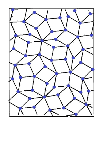
Figure 3. A Penrose tiling

7. Is $\mathbb{Z}^{d}_{\rm prim}$ a quasicrystal?

It is natural to ask whether $\mathbb{Z}^{d}_{\rm prim}$ is a quasicrystal. The answer is “No.” However $\mathbb{Z}^{d}_{\rm prim}$ is nearly a quasicrystal of Poisson type.

To see this, take a look again at the identity

$$\sum_{{\bf z}\in\mathbb{Z}^{d}_{\rm prim}}f({\bf z})=\sum_{k=1}^{\infty}\mu(k)\sum_{{\bf w}\in\mathbb{Z}^{d}\backslash\{{\bf 0}\}}f(k{\bf w}).$$

Suppose that ${\rm supp}~{}\!f\subset B_{N}({\bf 0})$. Then applying the Poisson summation formula, we obtain

$$\sum_{{\bf z}\in\mathbb{Z}^{d}_{\rm prim}}f({\bf z}) = \sum_{k=1}^{\infty}\mu(k)\sum_{{\bf w}\in\mathbb{Z}^{d}\backslash\{0\}}f(k{\bf w})$$

$$= \sum_{k=1}^{N}\mu(k)\Big{[}\sum_{{\bf w}\in\mathbb{Z}^{d}}f(k{\bf w})-f({\bf 0})\Big{]}$$

$$= \sum_{k=1}^{N}\mu(k)k^{-d}\sum_{\boldsymbol{\xi}\in k^{-1}\mathbb{Z}^{d}}\hat{f}(\boldsymbol{\xi})-\Big{(}\sum_{k=1}^{N}\mu(k)\Big{)}f({\bf 0}).$$

Now for $\boldsymbol{\xi}\in\mathbb{Q}^{d}$, we write

$$\boldsymbol{\xi}=\Big{(}\frac{b_{1}}{a_{1}},\ldots,\frac{b_{d}}{a_{d}}\Big{)},\quad{\rm gcd}(a_{i},b_{i})=1,a_{i}>0,$$

and put $n(\boldsymbol{\xi})={\rm lcm}(a_{1},\ldots,a_{d})$. Then $\boldsymbol{\xi}\in k^{-1}\mathbb{Z}^{d}~{}\Longleftrightarrow~{}n(\boldsymbol{\xi})|k$, and hence

$$\sum_{{\bf z}\in\mathbb{Z}^{d}_{\rm prim}}f({\bf z})=\sum_{k=1}^{N}\mu(k)k^{-d}\sum_{\boldsymbol{\xi}\in\mathbb{Q}^{d}\atop n(\boldsymbol{\xi})\mid k}\hat{f}(\boldsymbol{\xi})-\Big{(}\sum_{k=1}^{N}\mu(k)\Big{)}f({\bf 0}),$$

where we should note that the first term in the right-hand side is an absolutely convergent series. To rewrite the right-hand side further, consider

$$\mathbb{Q}^{d}_{N}=\{\boldsymbol{\xi}\in\mathbb{Q}^{d}|~{}\!n(\boldsymbol{\xi})\leq N\},$$

$$A=\{(k,\boldsymbol{\xi})|~{}\!k=1,\ldots,N,~{}\boldsymbol{\xi}\in\mathbb{Q}^{d},~{}n(\boldsymbol{\xi})|k\},$$

$$B=\{(\ell,\boldsymbol{\xi})|~{}\!1\leq\ell\leq Nn(\boldsymbol{\xi}){}^{-1},~{}\boldsymbol{\xi}\in\mathbb{Q}^{d}_{N}\}.$$

Then the map $(k,\boldsymbol{\xi})\mapsto(kn(\boldsymbol{\xi}){}^{-1},\boldsymbol{\xi})$ is a bijection of $A$ onto $B$. Therefore we get

$$\sum_{{\bf z}\in\mathbb{Z}^{d}_{\rm prim}}f({\bf z})=\sum_{\boldsymbol{\xi}\in\mathbb{Q}^{d}_{N}}\sum_{1\leq\ell\leq N/n(\boldsymbol{\xi})}\frac{\mu(\ell n(\boldsymbol{\xi}))}{(\ell n(\boldsymbol{\xi}))^{d}}\hat{f}(\boldsymbol{\xi})-\Big{(}\sum_{k=1}^{N}\mu(k)\Big{)}f({\bf 0}).$$

Clearly

$$\mu(\ell n(\boldsymbol{\xi}))=\begin{cases}\mu(\ell)\mu(n(\boldsymbol{\xi}))&({\rm gcd}(\ell,n(\boldsymbol{\xi}))=1)\\ 0&({\rm gcd}(\ell,n(\boldsymbol{\xi}))>1).\end{cases}$$

Therefore putting

$$a_{N}(\boldsymbol{\xi})=\frac{\mu(n(\boldsymbol{\xi}))}{n(\boldsymbol{\xi}){}^{d}}\sum_{1\leq\ell\leq N/n(\boldsymbol{\xi})\atop{\rm gcd}(\ell,n(\boldsymbol{\xi}))=1}\frac{\mu(\ell)}{\ell^{d}},$$

$$\Lambda_{N}=\{\boldsymbol{\xi}\in\mathbb{Q}^{d}_{N}|~{}\!\mu(n(\boldsymbol{\xi}))\neq 0\},$$

we get

$$\sum_{{\bf z}\in\mathbb{Z}^{d}_{\rm prim}}f({\bf z})=\sum_{\boldsymbol{\xi}\in\Lambda_{N}}a_{N}(\boldsymbol{\xi})\hat{f}(\boldsymbol{\xi})-\Big{(}\sum_{k=1}^{N}\mu(k)\Big{)}f({\bf 0}).$$

Furthermore, if we put

$$\Lambda=\{\boldsymbol{\xi}\in\mathbb{Q}^{d}|~{}\!\mu(n(\boldsymbol{\xi}))\neq 0\},$$

$$a(\boldsymbol{\xi})=\frac{\mu(n_{\boldsymbol{\boldsymbol{\xi}}})}{n(\boldsymbol{\xi}){}^{d}}\zeta(d)^{-1}\prod_{p|n(\boldsymbol{\xi})}\big{(}1-p^{-d}\big{)}^{-1}\quad(\boldsymbol{\xi}\in\Lambda),$$

then

$$\Lambda=\bigcup_{N=1}^{\infty}\Lambda_{N},\qquad\lim_{N\to\infty}a_{N}(\boldsymbol{\xi})=\frac{\mu(n(\boldsymbol{\xi}))}{n(\boldsymbol{\xi}){}^{d}}\sum_{\ell=1\atop{\rm gcd}(\ell,n(\boldsymbol{\xi}))=1}^{\infty}\frac{\mu(\ell)}{\ell^{d}}=a(\boldsymbol{\xi}).$$

This implies that if the “extra term” $\displaystyle\Big{(}\sum_{k=1}^{N}\mu(k)\Big{)}f({\bf 0})$ is ignored, then the set $\mathbb{Z}^{d}_{\rm prim}$ looks like a quasicrystal of Poisson type. This is the reason why we say that $\mathbb{Z}^{d}_{\rm prim}$ is nearly a quasicrystal of Poisson type.

Remark 7.1.

(1) Applying Eq. ​5.3, we obtain

$$\sum_{{\bf z}\in(\mathbb{Z}^{\rm odd})^{2}_{\rm prim}}f({\bf z})=\sum_{\boldsymbol{\xi}\in\mathbb{Q}_{2N}^{2}}\Big{(}\sum_{k\geq 1,h\geq 0\atop n(\boldsymbol{\xi})|k2^{h+1}}^{k2^{h}\leq N}\frac{\mu(k)}{k^{2}}\frac{1}{2^{2h+2}}e^{\pi ik2^{h+1}\langle\boldsymbol{\xi},{\bf 1}\rangle}\Big{)}\hat{f}(\boldsymbol{\xi}),$$

where ${\rm supp}~{}\!f\subset B_{N}({\bf 0})$ and ${\bf 1}=(1,1)$. This implies that $(\mathbb{Z}^{\rm odd})^{2}_{\rm prim}$ is a quasicrystal of Poisson type. The reason why no extra terms appear in this case is that $(\mathbb{Z}^{\rm odd})^{2}=2\mathbb{Z}^{2}+{\bf 1}$ is a full lattice.

(2) In much the same manner as above, we get

$$\sum_{{\bf z}\in\mathbb{Z}^{d}_{\rm prim}}f({\bf z})e^{2\pi i\langle{\bf z},\boldsymbol{\eta}\rangle}=\sum_{\boldsymbol{\xi}\in\Lambda_{N}}a_{N}(\boldsymbol{\xi})\hat{f}(\boldsymbol{\xi}-\boldsymbol{\eta})-\Big{(}\sum_{k=1}^{N}\mu(k)\Big{)}f({\bf 0}).$$

Using this identity, we can show

$$\lim_{\epsilon\to+0}\sigma(f^{\epsilon},\mathbb{Z}^{d}_{\rm prim},\omega_{\boldsymbol{\eta}})=a(\boldsymbol{\eta})\int_{\mathbb{R}^{d}}f({\bf x})~{}\!d{\bf x},$$

that is, $(\mathbb{Z}^{d}_{\rm prim},\omega_{\boldsymbol{\eta}})$ has constant density for $\boldsymbol{\eta}$ with $\mu(n(\boldsymbol{\eta}))\neq 0$.

(3) An interesting problem related to quasicrystals comes up in the study of non-trivial zeros of the Riemann zeta function (thus we come across another Riemann’s work, which were to change the direction of mathematical research in a most significant way).

We put

$$\Gamma^{\rm zero}=\{{\rm Im}~{}\!s\in\mathbb{R}|~{}\zeta(s)=0,~{}0<{\rm Re}~{}\!s<1\}.$$

Under the Riemann Hypothesis (RH), one may say that $\Gamma^{\rm zero}$ is nearly a quasicrystal of Poisson type of $1$-dimension (cf. ​Dyson ​[6]). Actually a version of Riemann’s explicit formula looks like a generalized Poisson formula (see Iwaniec and Kowalski [7]):

$$\sum_{\rho}f\left(\frac{\rho-1/2}{i}\right)=f\Big{(}\frac{1}{2i}\Big{)}+f\Big{(}-\frac{1}{2i}\Big{)}$$

$$+\frac{1}{2\pi}\int_{-\infty}^{\infty}f(u){\rm Re}\frac{\Gamma^{\prime}}{\Gamma}\Big{(}\frac{1}{4}+\frac{iu}{2}\Big{)}du$$

$$-\frac{1}{2\pi}\hat{f}(0)\log\pi-\frac{1}{2\pi}\sum_{m=1}^{\infty}\sum_{p}\frac{\log p}{p^{m/2}}\left(\hat{f}\Big{(}\frac{\log p^{m}}{2\pi}\Big{)}+\hat{f}\Big{(}-\frac{\log p^{m}}{2\pi}\Big{)}\right).$$

where $\{\rho\}$ is the set of zeros of $\zeta(s)$ with $0<{\rm Re}~{}\!\rho<1$, $\displaystyle\sum_{p}$ is the sum over all primes, and $\Gamma^{\prime}/\Gamma$ is the logarithmic derivative of the gamma function. Notice that, under the RH, the sum in the left-hand side is written as $\displaystyle\sum_{{\bf z}\in\Gamma^{\rm zero}}f({\bf z})$. What we should stress here is that the test function $f(s)$ is not arbitrary, and is supposed to be analytic in the strip $|{\rm Im}~{}\!s|\leq 1/2+\epsilon$ for some $\epsilon>0$, and to satisfy $|f(s)|\leq(1+|s|)^{-(1+\delta)}$ for some $\delta>0$ when $|{\rm Re}~{}\!s|\to\infty$. This restriction on $f$ together with the extra terms in the formula above says that $\Gamma^{\rm zero}$ is not a genuine quasicrystal of Poisson type. Furthermore $\Gamma^{\rm zero}$ does not have the Delone property. $\Box$

References

- [1] L. Comtet, Advanced Combinatorics: The Art of Finite and Infinite Expansions, Springer, 1974.
- [2] N. G. de Bruijn, Algebraic theory of Penrose’s nonperiodic tilings of the plane, I, II, Indagationes Mathematicae (Proceedings), 84 (1981), 39–52, 53–66.
- [3] N. G. de Bruijn, Quasicrystals and their Fourier transform, Indagationes Mathematicae (Proceedings), 89 (1986), 123–152.
- [4] B. N. Delone, Neue Darstellung der geometrischen Kristallographie, Z. Kristallographie 84 (1932), 109–149.
- [5] W. Duke, Rational points on the sphere, Ramanujan Journal, 7 (2003), 235–239.
- [6] F. Dyson, Birds and frogs, Notices of the AMS, 56 (2009), 212–223.
- [7] H. Iwaniec and E. Kowalski, Analytic number theory, Amer. Math. Soc. Colloq. Publ. 53 (American Mathematical Society, Providence, RI, 2004).
- [8] J. C. Lagarias, Mathematical quasicrystals and the problem of diffraction, Directions in Mathematical Quasicrystals, edited by Michael Baake and Robert V. Moody, American Mathematical Soc. (2000), 61–94.
- [9] D. N. Lehmer, Asymptotic evaluation of certain totient sums, Amer. J. Math. 22 (1900), 293–335.
- [10] J. Marklof and A. Strömbergsson, Visibility and directions in quasicrystals, Int. Math. Res. Not., first published online September 2, 2014 doi:10.1093/imrn/rnu140.
- [11] P. Mattila, Geometry of Sets and Measures in Euclidean Spaces: Fractals and Rectifiability, Cambridge University Press, 1999.
- [12] S. Ranganathan, On the geometry of coincidence-site lattices, Acta Cryst. 21 (1966), 197–199.
- [13] D. Shechtman, I. Blech, D. Gratias, and J. W. Cahn, Metallic phase with long-range orientational order and no translational symmetry, Phys. Rev. Lett. 53 (1984), 1951–1953.
- [14] M. Senechal and J. Taylor, Quasicrystals: The View from Les Houches, Math. Intel. 12 (1990), 54–64.
- [15] C. L. Siegel, A mean value theorem in geometry of numbers, Annals of Math., 46 (1945), 340–347.
- [16] M. Somos, http://grail.cba.csuohio.edu/ somos/rtritab.txt
- [17] T. Sunada, Topological Crystallography —with a view towards Discrete Geometric Analysis—, Springer 2012.
- [18] T. Sunada, Topics on mathematical crystallography, to appear in “Groups, Graphs and Random Walks,” ed. by T. Ceccherini-Silberstein, M. Salvatori, and Ecaterina Sava-Huss, to appear in London Mathematical Society Lecture Note, 2017.
- [19] I. M. Vinogradov, Elements of Number Theory, Mineola, NY: Dover Publications, 2003.
- [20] A. Weil, Number Theory, An approach through history from Hammurapi to Legendre, Birkhäuser, 1984.
- [21] H. Weyl, Über die Gleichverteilung von Zahlen mod. Eins, Math. Ann. 77 (1916), 313–352.
- [22] A. M. Yaglom and I. M. Yaglom, Challenging Mathematical Problems with Elementary Solutions, Vol I, Dover, 1987.
- [23] P. Zeiner, Symmetries of coincidence site lattices of the cubic lattice, Z. Kristallgr. 220 (2005), 915–925.