Outflows, infall and evolution of a sample of embedded low-mass protostars

Abstract

Context. Herschel observations of water and highly excited CO ($J>$9) have allowed the physical and chemical conditions in the more active parts of protostellar outflows to be quantified in detail for the first time. However, to date, the studied samples of Class 0/I protostars in nearby star-forming regions have been selected from bright, well-known sources and have not been large enough for statistically significant trends to be firmly established.

Aims. We aim to explore the relationships between the outflow, envelope and physical properties of a flux-limited sample of embedded low-mass Class 0/I protostars.

Methods. We present spectroscopic observations in H₂O, CO and related species with Herschel HIFI and PACS, as well as ground-based follow-up with the JCMT and APEX in CO, HCO⁺ and isotopologues, of a sample of 49 nearby ($d<$500 pc) candidate protostars selected from Spitzer and Herschel photometric surveys of the Gould Belt. This more than doubles the sample of sources observed by the WISH and DIGIT surveys. These data are used to study the outflow and envelope properties of these sources. We also compile their continuum spectral energy distributions (SEDs) from the near-IR to mm wavelengths in order to constrain their physical properties (e.g. $L_{\mathrm{bol}}$, $T_{\mathrm{bol}}$ and $M_{\mathrm{env}}$).

Results. Water emission is dominated by shocks associated with the outflow, rather than the cooler, slower entrained outflowing gas probed by ground-based CO observations. These shocks become less energetic as sources evolve from Class 0 to Class I. Outflow force, measured from low-$J$ CO, also decreases with source evolutionary stage, while the fraction of mass in the outflow relative to the total envelope (i.e. $M_{\mathrm{out}}/M_{\mathrm{env}}$) remains broadly constant between Class 0 and I. The median value of $\sim$1$\%$ is consistent with a core to star formation efficiency on the order of 50$\%$ and an outflow duty cycle on the order of 5$\%$. Entrainment efficiency, as probed by $F_{\mathrm{CO}}/\dot{M}_{\mathrm{acc}}$, is also invariant with source properties and evolutionary stage. The median value implies a velocity at the wind launching radius of 6.3 km s^-1, which in turn suggests an entrainment efficiency of between 30 and 60$\%$ if the wind is launched at $\sim$1AU, or close to 100$\%$ if launched further out. $L$[O i] is strongly correlated with $L_{\mathrm{bol}}$ but not with $M_{\mathrm{env}}$, in contrast to low-$J$ CO, which is more closely correlated with the latter than the former. This suggests that [O i] traces the present-day accretion activity of the source while CO traces time-averaged accretion over the dynamical timescale of the outflow. H₂O is more strongly correlated with $M_{\mathrm{env}}$ than $L_{\mathrm{bol}}$, but the difference is smaller than low-$J$ CO, consistent with water emission primarily tracing actively shocked material between the wind, traced by [O i], and the entrained molecular outflow, traced by low-$J$ CO. $L$[O i] does not vary from Class 0 to Class I, unlike CO and H₂O. This is likely due to the ratio of atomic to molecular gas in the wind increasing as the source evolves, balancing out the decrease in mass accretion rate. Infall signatures are detected in HCO⁺ and H₂O in a few sources, but still remain surprisingly illusive in single-dish observations.

1 Introduction

The general, cartoon picture of how stars form has been agreed for some time: a dense core within a molecular cloud becomes gravitationally unstable, causing material to fall inwards towards the centre; a protostar forms and launches a bi-polar molecular outflow; over time the outflow and infall combine to remove the envelope, eventually starving the protostar, which then slowly settles to the main sequence (e.g. Shu et al., 1987). However, a more detailed understanding is still required, particularly on infall and outflow, in order to quantitatively track the conversion of matter into stars and accurately predict the evolution and outcome of the star-formation process for individual sources, stellar clusters and even whole galaxies.

The first step is improved quantification of the basic physical properties (e.g. $L_{\mathrm{bol}}$, $M_{\mathrm{env}}$) and evolutionary state of low-mass protostars, on which considerable progress has been made. Improvements in detectors and telescopes have lead to full-wavelength coverage from optical to radio wavelengths at better sensitivity and resolution, while dedicated very long baseline interferometry (VLBI) campaigns in the radio are providing much more accurate distances for nearby star-forming regions (e.g. Loinard, 2013, for a recent review).

A framework for defining the evolutionary status of protostars has also been developed, dividing protostellar sources into one of five categories (Class 0, Class I, Flat, Class II and Class III) using various ways of quantifying the shift in the spectral energy distribution (SED) to shorter wavelengths as the source evolves: the infrared spectral index ($\alpha_{\mathrm{IR}}$, e.g. Lada & Wilking, 1984; Lada, 1987; Greene et al., 1994); the submillimetre ($\lambda>350$ $\mu$m) to bolometric luminosity ratio ($L_{\mathrm{submm}}/L_{\mathrm{bol}}$ used as a proxy for $M_{\mathrm{env}}/L_{\mathrm{bol}}$, e.g. André et al., 1993); and bolometric temperature ($T_{\mathrm{bol}}$, e.g. Myers & Ladd, 1993; Chen et al., 1995). For this latter measure, which is the intensity-weighted peak of the SED, these classifications are defined as: Class 0 ($T_{\mathrm{bol}}<70$ K), Class I (70$\leq T_{\mathrm{bol}}<$650 K), Class II (650$\leq T_{\mathrm{bol}}<$2800 K) and Class III ($T_{\mathrm{bol}}\geq$2800 K). Flat-SED sources have $T_{\mathrm{bol}}$ values in the 350$-$950 K range with a mean around 650 K (Evans et al., 2009).

The Spitzer Space Telescope (Gallagher et al., 2003) and more recently the Herschel Space Observatory (Pilbratt et al., 2010) have allowed the full potential of this evolutionary framework to be exploited in constraining how the properties of protostars change as the source evolves through large-area, high spatial resolution, uniform photometric surveys of many nearby star-forming regions (e.g. Evans et al., 2003, 2009; André et al., 2010; Rebull et al., 2010; Megeath et al., 2012; Dunham et al., 2014; Furlan et al., 2016). Furthermore, the statistics available from such large surveys have enabled estimates of the relative lifetimes of the different Classes to be obtained, showing in particular that the combined Class 0 and I phases, where the majority of the protostellar mass is accreted and the final properties of the star and its accompanying disk are imprinted, last approximately 0.4$-$0.7 Myr (Dunham et al., 2015; Heiderman & Evans, 2015; Carney et al., 2016).

For a 1$M_{\odot}$ star, such lifetimes imply typical time-averaged mass-accretion rates onto the protostar of approximately 10^-6$M_{\odot}$ yr^-1. Since not all material in the core will end up on the star, the infall rate in the envelope must presumably be higher than this by at least a factor of 2 or 3. Searches to quantify the infall in protostars have presented candidates using molecular line observations (e.g. Gregersen et al., 1997; Mardones et al., 1997) based on the doppler-shift of infalling material causing asymmetries in the line profile (Myers et al., 2000). However, confirming and quantifying infall in protostellar envelopes remains extremely challenging, limiting our understanding of the rate at which, and route by which, material reaches the disk and protostar, as well as how this changes with time and depends on the mass of the core/star.

Bipolar molecular outflows also play an important role in the evolution and outcome of star formation, as they remove mass from and inject energy into the envelope and surrounding material. However, the driving mechanism for protostellar outflows is still uncertain (e.g. Arce et al., 2007; Frank et al., 2014). A decrease in the driving force was measured between Class 0 and I sources, in addition to relations with $L_{\mathrm{bol}}$ and M_env, by Bontemps et al. (1996) using ground-based observations of CO. They attributed the decrease in outflow driving force with Class to a decrease in the accretion/infall rate as the source evolves. However, their study only included ten Class 0 sources, as few were known at the time.

Recent observations of H₂O and highly-excited CO using the Heterodyne Instrument for the Far-Infrared (HIFI; de Graauw et al., 2010) and Photodetector Array Camera and Spectrometer (PACS; Poglitsch et al., 2010) with Herschel have shown that these primarily trace active shocks related to the outflow and/or warm disk winds heated by ambipolar diffusion, rather than the entrained outflow as is accessible with ground-based CO observations (Nisini et al., 2010; Kristensen et al., 2013; Tafalla et al., 2013; Santangelo et al., 2013, 2014; Mottram et al., 2014; Yvart et al., 2016). The line-width and intensity in these tracers decreases between Class 0 and I while the excitation conditions ($T$,$N$,$n$) remain the same (Mottram et al., 2014; Manoj et al., 2013; Karska et al., 2013; Green et al., 2013a; Karska et al., 2014a; Matuszak et al., 2015). However, these studies have typically considered relatively small samples ($N\lesssim$30) of bright, well-known sources and so the statistical significance of trends with evolution and other source parameters has, in some cases, been low.

Two of the main surveys studying nearby Class 0/I protostars with Herschel were the “Water in star-forming regions with Herschel” (WISH) guaranteed time key program (van Dishoeck et al., 2011), which observed 29 Class 0/I protostars with HIFI and PACS plus ground-based follow-up, and the “Dust, Ice, and Gas in Time” (DIGIT) Herschel key program (Green et al., 2013a, 2016), which observed a further 13 Class 0/I protostars, primarily with full-scan PACS spectroscopy. Both the WISH and DIGIT surveys selected their samples to target well known, archetypal sources, ensuring success in detecting water, CO and other species and the availability of complementary data. As a result, these samples favoured luminous sources with particularly prominent and extended outflows, which may not be representative of the general population of protostars. In addition, both programs together only included a total of 42 low-mass sources split between Classes 0 and I, limiting the statistical significance of trends with evolution that might otherwise have been expected, for example between integrated intensity in water emission and $T_{\mathrm{bol}}$.

The motivation of the “William Herschel Line Legacy” (WILL) survey was therefore to further explore the physics (primarily infall and outflow) and chemistry of water, CO and other complementary species in Class 0/I protostars in nearby low-mass star forming regions using a combination of Herschel and ground-based observations, building on WISH and DIGIT. The aim was to increase the number of Class 0/I protostars observed, thus improving the statistical significance of the existing correlations found by for example Kristensen et al. (2012), and allowing shallower correlations to be tested, as well as improving the sampling of fainter and colder sources.

This paper is structured as follows. Section 2 discusses the selection of the WILL sample, the basic physical properties of the sources and evaluates the properties of the combined WISH+DIGIT+WILL sample. Section 3 gives the details and basic results of both the Herschel observations and a complementary ground-based follow-up campaign. More detailed results and analysis are then presented thematically, centred around outflows (Sect. 4) and envelope emission (Sect. 5), followed by a discussion on the variation of water with evolution (Sect. 6). Finally, we summarise our main conclusions in Sect. 7.

2 Sample

2.1 Selection

The starting point for selecting a flux-limited sample of low-mass protostars was the catalogue of Class 0/I protostars identified as part of photometric surveys with the Spitzer Space Telescope of the closest major star-forming clouds that make up the Gould Belt (Gould, 1879). In particular, these were drawn from the Spitzer c2d (Evans et al., 2009), Spitzer Gould Belt (Dunham et al., 2015) and Taurus Spitzer (Rebull et al., 2010) surveys.

The initial catalogue was compiled from individual cloud catalogues for the Perseus, Taurus, Ophiuchus, Scorpius (also known as Ophiuchus North), Corona Australis and Chameleon star-forming regions (for more details, see Jørgensen et al., 2007; Rebull et al., 2007, 2010; Padgett et al., 2008; Jørgensen et al., 2008; Hatchell et al., 2012; Peterson et al., 2011; Alcalá et al., 2008). At the time of selection in 2011, the Herschel Gould Belt (André et al., 2010) survey had also produced catalogues of protostellar candidates in the Aquila Rift region (Maury et al., 2011), so these were also considered in an attempt to extend the coverage of the WILL survey to particularly young (cold) embedded young stellar objects (YSOs).

From this master catalogue of protostars in major star-forming regions within 500 pc, the following criteria were used to select the final WILL sample:

1. infrared slope (2$-$24 $\mu$m) $\alpha_{\mathrm{IR}}>$ 0.3 or non-detection,

2. $T_{\mathrm{bol}}<$ 350 K,

3. $L_{\mathrm{bol}}$ $>$ 0.4 $L_{\odot}$ for Class 0 ($T_{\mathrm{bol}}<$ 70 K),
   $L_{\mathrm{bol}}\geq$ 1 $L_{\odot}$ for Class I (70 $\leq T_{\mathrm{bol}}<$ 350 K),

4. $\delta$ $<$ 35^∘.

The distinction between Class I and II sources is normally made at $T_{\mathrm{bol}}$=650 K (Chen et al., 1995), however Evans et al. (2009) found that Flat SED sources cover the range 350$-$950 K with a mean around 650 K and therefore likely consist of more evolved Class I or younger Class II sources. An upper limit of 350 K was therefore imposed in order to exclude more evolved Class I sources from the sample. Water emission is typically weaker for Class I sources than Class 0s and is generally higher for more luminous sources (e.g. Kristensen et al., 2012), so a higher $L_{\mathrm{bol}}$ cut was used for Class I sources in an attempt to ensure detections. Criteria i$-$iii were therefore designed to ensure that the sample includes only young, deeply embedded protostars that are bright enough to be detected in H₂O and related species based on the experience of the WISH and DIGIT surveys. Criterion iv ensures that all WILL sources can be observed with ALMA to allow high spectral and spatial resolution ground-based interferometric follow-up of interesting sources.

Unfortunately, edge-on disks, reddened background sources and evolved asymptotic giant-branch (AGB) stars all have the potential to present similar infrared colours and thus contaminate any sample selected purely based on continuum properties. As first highlighted by van Kempen et al. (2009) for a sample of sources in Ophiuchus, molecular emission tracing dense gas can help to break this degeneracy. More specifically, the high critical density of HCO⁺ $J$=4$-$3 or $J$=3$-$2 means it will not be strong in foreground cloud material, while the rarity of C¹⁸O similarly means that the $J$=3$-$2 transition is only bright and concentrated in protostellar sources. In addition, more evolved disk sources will not present strong emission in single-dish HCO⁺ spectra due to beam-dilution. Such data, particularly for HCO⁺, have been collected and used to remove contaminants in a number of Gould Belt samples by Heiderman et al. (2010), Heiderman & Evans (2015) and Carney et al. (2016), which have some overlap with the initial candidate sample. Therefore, following the cuts detailed above, non-detection in HCO⁺ $J$=4$-$3 or 3$-$2 was used, where data were available, to exclude contaminant sources.

Most of the sources observed by the WISH and DIGIT surveys also conform to the above criteria, so any initial candidates within 5^′′ of a WISH or DIGIT source were also excluded to avoid repeat observations. However, two sources, PER 03 and PER 11, have enough overlap with the WISH observations of L1448-MM (offset by 7.7^′′) and NGC1333-IRAS4B (offset by 6.4^′′), respectively, particularly in the H₂O 1${}_{10}-$1₀₁ (557 GHz) ground-state line obtained in a 39^′′ beam, that they are removed from the WILL sample as presented here. Finally, source TAU 05 was removed as it is the young and active Class II source DG Tau B, which has an edge-on disk (Podio et al., 2013).

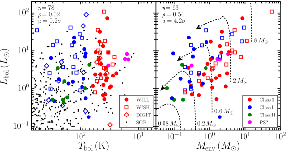
Figure 1: Top: The distribution of $L_{\mathrm{bol}}$ vs. $T_{\mathrm{bol}}$ and $M_{\mathrm{env}}$ for the WILL (filled circles), WISH (open squares) and DIGIT (open diamonds) surveys. In the left-hand panel, the Spitzer Gould Belt (SGB) determinations from Dunham et al. (2015) are shown for comparison (black dots). The different colours are used to distinguish between different source classifications: Class 0 (red), Class I (blue) Class II (green) and pre-stellar (PS, magenta). The number of sources ($n$), Pearson correlation coefficient ($\rho$), and the probability ($p$) that the correlation is not just due to random distributions in the variables are shown in the upper-left of each panel including only Class 0/I sources. Evolutionary tracks between $L_{\mathrm{bol}}$ and $M_{\mathrm{env}}$ from Duarte-Cabral et al. (2013) are shown in the right-hand panel (see text for details), with the final stellar mass indicated for each track. Bottom: histograms showing the distribution of $L_{\mathrm{bol}}$, $T_{\mathrm{bol}}$ and $M_{\mathrm{env}}$ for the WILL (blue), combined WISH and DIGIT (magenta hatched), and total WILL, WISH and DIGIT (black) samples. The grey shaded region indicates the distribution of the Spitzer Gould Belt determinations for sources with $T_{\mathrm{bol}}\leq$350 K.

2.2 Properties and evaluation

The properties of the final sample of 49 sources that make up the WILL sample are presented in Table 1. For simplicity, we give each a name based on the region and a number ordered by right ascension, but many are already well known and therefore the table also gives details of common names used by previous studies for the same sources.

The following distances are used for the various regions covered by our sample: 235 pc for Perseus (Hirota et al., 2008), 140 pc for Taurus (Kenyon et al., 2008), 125 pc for Ophiuchus and Scorpius (de Geus et al., 1989), 130 pc for Corona Australis (Knude & Høg, 1998), 150 pc for Chameleon I and 178 pc for Chameleon II (Whittet et al., 1997). For Aquila, W40 and Serpens South, Ortiz-León et al. (2016) recently found that these regions, as well as Serpens Main, are at a common distance of 436 pc.

The determination of the source properties and evolutionary classification is discussed in detail in Appendix A. To summarise briefly, the SED for each source is constructed from the near-IR to (sub-)mm and used to calculate $L_{\mathrm{bol}}$, $L_{\mathrm{submm}}$/$L_{\mathrm{bol}}$, $T_{\mathrm{bol}}$ and $\alpha_{\mathrm{IR}}$. $M_{\mathrm{env}}$ is obtained from sub-mm or mm photometry assuming that the dust is optically thin, while $\varv_{\mathrm{LSR}}$ is calculated from molecular line observations. Finally, the classification of each source is reached by considering the spatial and spectral properties of both the gas and dust associated with each source (see Appendix A.7 for more details).

The sample comprises 23 Class 0, 14 Class I, 8 Class II and 4 uncertain, potentially pre-stellar sources. In the case of this last group of sources, all in W40, they are faint or not detected at $<$160 $\mu$m, show few detections in PACS and have no indications of outflow activity, but the presence of the W40 PDR, detected in some of the HIFI and ground-based lines, leaves some ambiguity. These and other cases of note are discussed in more detail in Appendix C.

Table 1: The WILL survey source sample.

Name	RA ($J$2000)	Dec ($J$2000)	$d$	$\varv_{\mathrm{LSR}}$	$L_{\mathrm{bol}}$	$\frac{L_{\mathrm{submm}}}{L_{\mathrm{bol}}}$	$T_{\mathrm{bol}}$	$\alpha_{\mathrm{IR}}$	$M_{\mathrm{env}}$	Class	Other names
	(h m s)	(° ′ ′′)	(pc)	(km s-1)	($L_{\odot}$)	($\%$)	(K)		($M_{\odot}$)
AQU 01	18:29:03.82	$-$01:39:01.5	436	$+$7.4	02.6	11.8	024	$-$	3.15	0	Aqu-MM2
AQU 02	18:29:08.60	$-$01:30:42.8	436	$+$7.5	09.0	07.8	033	$-$	2.17	0	Aqu-MM4, IRAS 18265-0132
AQU 03	18:30:25.10	$-$01:54:13.4	436	$+$7.1	03.5	05.3	246	0.7	0.79	II	Aqu-MM6, IRAS 18278-0156
AQU 04	18:30:28.63	$-$01:56:47.7	436	$+$7.6	06.5	04.5	320	0.5	1.21	I	Aqu-MM7, IRAS 18278-0158
AQU 05	18:30:29.03	$-$01:56:05.4	436	$+$7.3	02.4	09.2	037	1.4	0.68	0	Aqu-MM10
AQU 06	18:30:49.94	$-$01:56:06.1	436	$+$8.3	01.3	08.2	040	1.9	0.59	0	Aqu-MM14
CHA 01	11:09:28.51	$-$76:33:28.4	150	$+$4.9	01.6	$-$	189	1.6	$-$	II	GM Cha, ISO-ChaI 192, CaINa2
CHA 02	12:59:06.58	$-$77:07:39.9	178	$+$3.0	01.8	00.6	236	1.3	$-$	I	ISO-ChaII 28, IRAS 12553-7651
CRA 01	19:02:58.67	$-$37:07:35.9	130	$+$5.6	02.4	02.2	055	1.7	0.49	0	ISO-CrA 182, IRAS 18595-3712
OPH 01	16:26:59.10	$-$24:35:03.3	125	$+$3.8	04.3	$-$	069	2.0	0.17	II+PDR?	ISO-Oph 90, WL 22
OPH 02	16:32:00.99	$-$24:56:42.6	125	$+$4.2	08.6	00.1	080	1.8	0.09	I	ISO-Oph 209, Oph-emb 10
PER 01	03:25:22.32	+30:45:13.9	235	$+$4.1	04.5	02.7	044	2.3	0.89	0	L1448 IRS2, Per-emb 22
PER 02	03:25:36.49	+30:45:22.2	235	$+$4.5	09.2	01.7	054	2.6	3.48	0	L1448 N(A), L1448 IRS3, Per-emb 33
PER 04	03:26:37.47	+30:15:28.1	235	$+$5.2	01.2	04.2	060	1.2	0.29	0	IRAS 03235+3004, Per-emb 25
PER 05	03:28:37.09	+31:13:30.8	235	$+$7.3	11.1	00.6	084	2.2	0.36	I	NGC1333 IRAS1, Per-emb 35
PER 06	03:28:57.36	+31:14:15.9	235	$+$7.3	07.1	$-$	082	1.5	0.34	I	NGC1333 IRAS2B, Per-emb 36
PER 07	03:29:00.55	+31:12:00.8	235	$+$7.4	00.7	03.9	037	2.1	0.32	0	Per-emb 3
PER 08	03:29:01.56	+31:20:20.6	235	$+$7.7	16.9	01.3	129	2.5	0.83	I	Per-emb 54, NGC1333 IRAS6
PER 09	03:29:07.78	+31:21:57.3	235	$+$7.5	22.7	$-$	129	2.6	0.26	I	IRAS 03260+3111(W), Per-emb 50
PER 10	03:29:10.68	+31:18:20.6	235	$+$8.7	06.0	02.2	047	1.9	1.10	0	NGC1333 IRAS7, Per-emb 21
PER 12	03:29:13.54	+31:13:58.2	235	$+$7.8	01.1	08.7	031	2.4	1.20	0	NGC1333 IRAS4C, Per-emb 14
PER 13	03:29:51.82	+31:39:06.0	235	$+$8.0	00.7	05.0	040	3.5	0.49	0	IRAS 03267+3128, Per-emb 9
PER 14	03:30:15.14	+30:23:49.4	235	$+$6.2	01.8	01.6	088	1.8	0.15	I	IRAS 03271+3013, Per-emb 34
PER 15	03:31:20.98	+30:45:30.1	235	$+$6.9	01.6	05.8	036	1.2	1.16	0	IRAS 03282+3035, Per-emb 5
PER 16	03:32:17.96	+30:49:47.5	235	$+$7.0	01.1	13.3	029	1.0	2.88	0	IRAS 03292+3039, Per-emb 2
PER 17	03:33:14.38	+31:07:10.9	235	$+$6.6	00.2	$-$	071	2.4	1.94	I	B1 SMM3, Per-emb 6
PER 18	03:33:16.44	+31:06:52.5	235	$+$6.6	00.5	$-$	038	1.6	1.59	0	B1d, Per-emb 10
PER 19	03:33:27.29	+31:07:10.2	235	$+$6.8	01.1	01.7	093	1.9	0.29	I	B1 SMM11, Per-emb 30
PER 20	03:43:56.52	+32:00:52.8	235	$+$8.9	02.2	06.3	027	0.7	1.93	0	IRAS 03407+3152, HH 211, Per-emb 1
PER 21	03:43:56.84	+32:03:04.7	235	$+$8.8	01.9	03.8	035	1.5	1.54	0	IC348 MMS, Per-emb 11
PER 22	03:44:43.96	+32:01:36.2	235	$+$9.8	02.4	03.4	045	0.9	0.70	0	IRAS 03415+3152, Per-emb 8
SCO 01	16:46:58.27	$-$09:35:19.8	125	$+$3.6	00.5	00.6	201	0.9	0.10	II	IRAS 16442-0930, L260 SMM1
SERS 01	18:29:37.70	$-$01:50:57.8	436	$+$8.2	17.4	03.9	046	1.3	1.10	0	IRAS 18270-0153, SerpS-MM1
SERS 02	18:30:04.13	$-$02:03:02.1	436	$+$7.8	73.2	04.6	034	2.5	8.44	0	SerpS-MM18
TAU 01	04:19:58.40	+27:09:57.0	140	$+$6.8	01.5	03.3	136	1.4	0.27	I	IRAS 04169+2702
TAU 02	04:21:11.40	+27:01:09.0	140	$+$6.6	00.5	00.8	282	0.5	$-$	I	IRAS 04181+2654A
TAU 03	04:22:00.60	+26:57:32.0	140	$+$7.4	00.4	00.2	196	1.0	$-$	II	IRAS 04189+2650(W)
TAU 04	04:27:02.60	+26:05:30.0	140	$+$6.3	01.4	01.5	161	0.8	0.64	I	DG TAU B
TAU 06	04:27:57.30	+26:19:18.0	140	$+$7.2	00.6	02.7	080	0.8	0.09	I	HH31 IRS 2, IRAS 04248+2612
TAU 07	04:29:30.00	+24:39:55.0	140	$+$6.3	00.6	00.2	169	0.9	$-$	II	HH 414, IRAS 04264+2433
TAU 08	04:32:32.00	+22:57:26.0	140	$+$5.5	00.5	01.2	300	0.5	0.18	II	L1536 IRS, IRAS 04295+2251
TAU 09	04:35:35.30	+24:08:19.0	140	$+$5.5	01.0	01.7	082	1.4	0.06	II	L1535 IRS, IRAS 04325+2402
W40 01	18:31:09.42	$-$02:06:24.5	436	$+$4.9	13.3	07.4	040	2.3	1.97	0+PDR	W40-MM3
W40 02	18:31:10.36	$-$02:03:50.4	436	$+$4.8	32.6	03.7	046	4.6	2.25	0	W40-MM5
W40 03	18:31:46.54	$-$02:04:22.5	436	$+$6.4	08.3	20.6	015	$-$	3.37	PS?+PDR	W40-MM26
W40 04	18:31:46.78	$-$02:02:19.9	436	$+$6.7	06.1	09.4	016	$-$	1.69	PS?+PDR	W40-MM27
W40 05	18:31:47.90	$-$02:01:37.2	436	$+$6.5	05.9	27.3	014	$-$	1.97	PS?+PDR	W40-MM28
W40 06	18:31:57.24	$-$02:00:27.7	436	$+$6.6	04.1	02.2	033	$-$	0.31	PS?+PDR	W40-MM34
W40 07	18:32:13.36	$-$01:57:29.6	436	$+$7.4	03.6	03.3	036	0.9	0.25	0	W40-MM36

Figure 1 shows the $L_{\mathrm{bol}}$, $T_{\mathrm{bol}}$ and $M_{\mathrm{env}}$ distribution of the WILL sample, along with the WISH and DIGIT samples for comparison. The properties of the WISH sample are taken from Kristensen et al. (2012) while those for the DIGIT sample are taken from Green et al. (2013a) and Lindberg et al. (2014). These are corrected to the distances for the various regions discussed above where needed. It should be noted that $M_{\mathrm{env}}$ values are not available for the DIGIT sample, leading to the difference in the number of sources between the upper-left and upper-right panels.

The probability (p) that a given value of the Pearson correlation coefficient ($\rho$) for sample size $n$ represents a real correlation (i.e. the likelihood that a two-tailed test can reject the null-hypothesis that the two variables are uncorrelated with $\rho$=0) can be expressed in terms of the standard deviation of a normal distribution, $\sigma$, as:

$$p=\mid\rho\mid\sqrt{n-1}\sigma,$$ (1)

following (Marseille et al., 2010). We consider $p=$3$\sigma$ (i.e. 99.7$\%$) to be the threshold for statistical significance. Thus, for a sample size of 30, values of $\mid\rho\mid>0.56$ indicate real, statistically significant correlations while for a sample size of 50, this is true for $\mid\rho\mid>0.43$. While one might expect correlations between some of the observed properties of embedded protostars due to the related nature of their different components (e.g. envelope, outflow and driving source), such tests are a simple way of ascertaining whether or not the data are able to support such links. As mentioned above, the extension of the sample of sources studied in spectral lines with PACS and HIFI enabled by the WILL survey and presented here allows us to study these more completely for the first time.

The evolutionary tracks between $L_{\mathrm{bol}}$ and M_env shown in the top-right panel of Figure 1 are taken from Duarte-Cabral et al. (2013). They assume an exponential decrease of $M_{\mathrm{env}}$ and a core-to-star formation efficiency of 50$\%$, such that the net accretion rate is given by:

$$\dot{M}_{\mathrm{acc}}(t)\leavevmode\nobreak\ =\leavevmode\nobreak\ 0.5\,\frac{M_{\mathrm{env}}(t)}{\tau}\,,$$ (2)

where $\tau$ is the e-folding time, which is assumed to be 3$\times$10⁵ yrs.

The WILL sample doubles the number of low-mass YSOs observed, which have slightly lower values of $L_{\mathrm{bol}}$ and $M_{\mathrm{env}}$, as well as lower $T_{\mathrm{bol}}$ for Class 0 sources, than the WISH and DIGIT samples. Comparing to Spitzer Gould Belt (SGB) sources with $T_{\mathrm{bol}}\leq$350 K, taken from Dunham et al. (2015), it can be seen in Fig. 1 that the combined WILL+DIGIT+WISH sample is representative of the overall Class 0/I population and contains most sources above $\sim$1$L_{\odot}$. Below this luminosity, the sample rapidly becomes incomplete, and thus the combined sample is still biased towards higher mean $L_{\mathrm{bol}}$ compared with the general distribution, but the addition of the WILL sources shifts the completeness limit approximately a factor of three lower. In terms of $T_{\mathrm{bol}}$, the sample is biased towards lower values, but judging from upper-left panel of Fig. 1, the higher $T_{\mathrm{bol}}$ sources in the SGB data are primarily those below our $L_{\mathrm{bol}}$ limit, that is, the mean $L_{\mathrm{bol}}$ decreases as $T_{\mathrm{bol}}$ increases for SGB sources. The differences between the values of Dunham et al. (2015) and those given here for individual sources are likely due to our inclusion of far-IR data in these determinations.

It is worth mentioning a couple of caveats. Firstly, the sample of Class 0 sources is dominated by sources in the Perseus molecular cloud, while the Class I sources are drawn from a number of regions that vary in the concentration and activity of their star formation (e.g. Taurus vs. Ophiuchus). There may well be regional differences due to environmental effects, which we cannot test due to the overall small sample size for a given region. Secondly, by excluding older Class I and flat-spectrum sources, we introduce a bias towards younger Class I sources, so the properties of an average Class I source may well be slightly different from those determined with this sample. However, in general for the part of parameter space that WILL, WISH and DIGIT are designed to probe, the addition of the WILL survey leaves the combined sample broadly complete.

3 Observations and results

The primary observations for the WILL survey were taken with Herschel using the Heterodyne Instrument for the Far-Infrared (HIFI, de Graauw et al., 2010) and Photodetector Array Camera and Spectrometer (PACS, Poglitsch et al., 2010) detectors between the 31^st October 2012 and 27^th March 2013. The observing modes, observational properties, data reduction and detection statistics are described for each instrument separately in Sections 3.1 and 3.2. Complementary spectroscopic maps obtained through follow-up observations of the sample with ground-based facilities are then described in Section 3.3.

3.1 HIFI

3.1.1 Observational details

HIFI was a set of seven single-pixel dual-sideband heterodyne receivers that combined to cover the frequency ranges 480$-$1250 GHz and 1410$-$1910 GHz with a sideband ratio of approximately unity. Spectra were simultaneously observed in two polarisations, $H$ and $V$, which pointed at slightly different positions on the sky ($\sim$6.5^′′ apart at 557 GHz decreasing to $\sim$2.8^′′ at 1153 GHz), with two spectrometers simultaneously providing both wideband (WBS, 4 GHz bandwidth at 1.1 MHz resolution) and high-resolution (HRS, typically 230 MHz bandwidth at 250 kHz resolution) frequency coverage.

The HIFI component of the WILL Herschel observations consists of single pointed spectra at four frequency settings, principally targeting the H₂O 1${}_{10}-$1₀₁, 1${}_{11}-$0₀₀ and 2${}_{02}-$1₁₁ transitions at 557, 1113 and 988 GHz respectively and the ¹²CO $J$=10$-$9 transition at 1152 GHz, which also includes the H₂O 3${}_{12}-$2₂₁ transition. All observations were carried out in dual-beam-switch mode with a nod of 3^′ using fast chopping. The specific central frequencies of the settings were chosen to maximise the number of observable H₂O, CO and H${}_{2}^{18}$O transitions, the details of which are given in Table LABEL:T:observations_hifi_lines along with the corresponding instrumental properties, spectral and spatial resolution, and observing time. The main difference compared to the WISH HIFI observations of low-mass sources (see Kristensen et al., 2012; Mottram et al., 2014) was that the frequency of the WILL observations for the H₂O 1${}_{10}-$1₀₁ and 1${}_{11}-$0₀₀ settings was set so that the corresponding H${}_{2}^{18}$O transition was observed simultaneously, and longer observing times were used for the H₂O 1${}_{10}-$1₀₁ setting. The observation ID numbers for all WILL HIFI observations are given in Table B.14.

Table 2: Principle lines observed with HIFI.

Species	Transition	Rest Frequency	$E_{\mathrm{u}}$/$k_{\mathrm{b}}$	$A_{\mathrm{ul}}$	$n_{\mathrm{cr}}$	$\eta_{mb}$	$\theta_{mb}$	WBS resolution	HRS resolution	Obs. Time	Det.
		(GHz)	(K)	(s-1)	(cm-3)	(H/V)	(′′)	( km s-1)	( km s-1)	(min)
o-H2O	110-101	0556.93599	061.0	3.46$\times$10-3	1$\times$107	0.62/0.62	38.1	0.27	0.03	38	39/46
	312-221	1153.12682	249.4	2.63$\times$10-3	8$\times$106	0.59/0.59	18.4	0.13	0.06	13	07/46
p-H2O	111-000	1113.34301	053.4	1.84$\times$10-2	1$\times$108	0.63/0.64	19.0	0.13	0.06	28	28/46
	202-111	0987.92676	100.8	5.84$\times$10-3	4$\times$107	0.63/0.64	21.5	0.15	0.07	36	25/46
o-H${}_{2}^{18}$O	110-101	0547.67644	060.5	3.29$\times$10-3	1$\times$107	0.62/0.62	38.7	0.27	0.07	38	01/46
p-H${}_{2}^{18}$O	111-000	1101.69826	052.9	1.79$\times$10-2	1$\times$108	0.63/0.64	19.0	0.13	0.06	28	00/46
C18O	9$-$8	0987.56038	237.0	6.38$\times$10-5	2$\times$105	0.63/0.64	21.5	0.15	0.07	36	04/46
CO	10$-$9	1151.98545	304.2	1.01$\times$10-4	3$\times$105	0.59/0.59	18.4	0.13	0.06	13	40/46
13CO	10$-$9	1101.34966	290.8	8.86$\times$10-5	3$\times$105	0.63/0.64	19.3	0.13	0.06	28	20/46

Initial data reduction was conducted using the Herschel Interactive Processing Environment (hipe v. 10.0, Ott, 2010). After initial spectrum formation, any instrumental standing waves were removed. Next, a low-order ($\leq$2) polynomial baseline was subtracted from each sub-band. The fit to the baseline was then used to calculate the continuum level, compensating for the dual-sideband nature of the HIFI detectors (the initial continuum level is the combination of emission from both the upper and lower sideband, which we assume to be equal). Following this the WBS sub-bands were stitched into a continuous spectrum and all data were converted to the $T_{\mathrm{MB}}$ scale using the latest beam efficiencies (see Table LABEL:T:observations_hifi_lines). Finally, for ease of analysis, all data were converted to FITS format and resampled to 0.3 km s^-1 spectral resolution on the same velocity grid using bespoke python routines.

Few differences have been found in line-shape or gain between the $H$ and $V$ polarisations (e.g. Kristensen et al., 2012; Yıldız et al., 2013; Mottram et al., 2014), so after visual inspection the two polarisations were co-added to improve signal-to-noise. The velocity calibration is better than 100 kHz, while the pointing uncertainty is better than 2^′′ and the intensity calibration uncertainty is $\lesssim$10$\%$ (Mottram et al., 2014).

3.1.2 Results

Figures 2 and 3 present the observed HIFI ortho-H₂O 1${}_{10}-$1₀₁ (557 GHz) ground-state transition and ¹²CO $J$=10$-$9, respectively, for all WILL sources. The water spectra are complex, containing multiple components, some absorption, which is usually narrow, and emission up to $\pm\sim$100 km s^-1 from the source velocity, similar to other Herschel HIFI observations of water towards Class 0/I sources (e.g. Kristensen et al., 2012). ¹²CO $J$=10$-$9 typically shows two gaussian emission components with a lower total velocity extent than H₂O. Strong, narrow absorption in ¹²CO $J$=10$-$9 for W40 sources 01, 03 and 06 (see Fig. 3) indicates that contamination in at least one of the reference positions affects these spectra and also likely affects most of the H₂O transitions for these sources as well. The narrow yet bright nature of the ¹²CO $J$=10$-$9 seen in six sources (OPH 01, W40 01 and W40 03$-$06, see Fig. 3), combined with the narrow and low-intensity nature of the H₂O emission, suggests that they are related to photon-dominated regions (PDRs, c.f. for example CO observations of the Orion Bar PDR, Hogerheijde et al., 1995; Jansen et al., 1996; Nagy et al., 2013).

The detection statistics for all transitions are given in the last column of Table LABEL:T:observations_hifi_lines, excluding W40 sources 01, 03 and 06 due to the contamination of these spectra. The H₂O 1${}_{10}-$1₀₁ transition is detected towards 39/46 sources in total, including 33/36 confirmed Class 0/I sources (not detected in CHA 02, PER 04 and W40 07, see Fig. 2), while ¹²CO $J$=10$-$9 is detected towards 40/46 sources in total including 32/36 Class 0/Is (not detected in CHA 02, PER 07, PER 15 and W40 07). H${}_{2}^{18}$O 1${}_{10}-$1₀₁ is only detected towards the source with the strongest H₂O emission, SERS 02, while C¹⁸O $J$=9$-$8 is only detected towards four sources (PER 02, SERS 02, W40 04 and  05).

A more detailed analysis of the kinematics of the HIFI lines is presented and discussed in San José-García (2015), including the results of Gaussian decomposition of the lines using the methods outlined for the WISH sample by Mottram et al. (2014) and San José-García et al. (2013) for H₂O and CO, respectively. In summary, the minimum number of Gaussian components is found that results in no residuals above 3$\sigma$, with these components then categorised between the envelope and C or J-type outflow-related shocks depending on their width and offset from the source velocity. A global fit is used for the H₂O transitions with the component peak velocity and line-widths constrained by all lines and the intensity allowed to vary between transitions because the lines all have a consistent shape. The different CO transitions are fit independently as their line profile shapes vary between different transitions.

Figure 2: H₂O 1${}_{10}-$1₀₁ (557 GHz) continuum-subtracted spectra for the final WILL sample. All have been recentred so that the source velocity is at zero. The number in the upper-right corner of each panel indicates what factor the spectra have been multiplied by in order to show them on a common scale.

Figure 3: CO $J$=10$-$9 continuum-subtracted spectra for the final WILL sample. All have been recentred so that the source velocity is at zero. The number in the upper-right corner of each panel indicates what factor the spectra have been multiplied by in order to show them on a common scale.

3.2 PACS

3.2.1 Observational details

PACS consisted of four detectors, two photoconductor arrays with 16$\times$25 pixels for integral field unit (IFU) spectroscopy and two bolometer arrays with 16$\times$32 and 32$\times$64 pixels for broad-band imaging photometry. In IFU spectroscopy mode, observations were taken simultaneously in the red 1st order grating (102$-$210 $\mu$m) and one of the 2nd or 3rd order blue gratings (51$-$73 $\mu$m or 71$-$105 $\mu$m) over 5$\times$5 spatial pixels (spaxels), which covered a 47^′′$\times$47^′′ field of view. For details of the 70, 100 and 160 $\mu$m PACS (and 250, 350 and 500 $\mu$m SPIRE, Griffin et al., 2010) photometric maps used to determine the continuum flux densities for the SEDs (discussed in Section A.1) see André et al. (2010).

Table 3: Wavelength ranges covered by WILL PACS line-scan settings.

Setting	Wavelengths	Primary Transitions
	( $\mu$m)
1	078.6 $-$ 079.5	H2O 4${}_{23}-$312, 6${}_{15}-$524, CO 33$-$32, OH
	081.3 $-$ 082.2	H2O 6${}_{16}-$505, CO 32$-$31
	084.2 $-$ 085.0	H2O 7${}_{16}-$707, CO 31$-$30, OH
	089.5 $-$ 090.4	H2O 3${}_{22}-$211, CO 29$-$28
	123.7 $-$ 126.1	H2O 4${}_{04}-$313, CO 21$-$20
	157.0 $-$ 158.0	[C ii]
	162.5 $-$ 164.5	CO 16$-$15, OH
	168.3 $-$ 170.0
	179.0 $-$ 180.8	H2O 2${}_{12}-$101, 2${}_{21}-$212
2	053.6 $-$ 055.0
	063.0 $-$ 063.5	H2O 8${}_{18}-$707, [O i]
	107.3 $-$ 109.7	H2O 2${}_{21}-$110, CO 24$-$23
	189.0 $-$ 190.5

WILL PACS observations were carried out using the IFU in line-scan mode where deep observations were obtained for targeted wavelength regions (bandwidth $\Delta\lambda/\lambda$=0.01) around selected transitions. Two wavelength settings were used, each including observations in both the blue and red gratings, as summarised in Table LABEL:T:observations_pacs_settings. The principle transitions within these regions are from H₂O, OH, [O i], CO and [C ii], the properties of which are given in Table LABEL:T:observations_pacs_lines. While WILL targeted the key lines observed by WISH, some of the wavelength ranges were shifted slightly in order to allow for better baseline subtraction or additional line detections (e.g. those around 82 and 90 $\mu$m were shifted to slightly longer wavelengths) while others were omitted to save time (e.g. around CO $J$=14-13). The velocity resolution of PACS ranges from 75 km s^-1 at the shortest wavelength to 300 km s^-1, with only [O i] sometimes showing velocity resolved line profiles in a few sources. All observations used a chopping/nodding observing mode with off-positions within 6^′ of the target coordinates. The obsids for WILL PACS observations are given in Table B.14. For one source, TAU 08, PACS data were not obtained because the coolant on Herschel ran out before they could be successfully observed.

Data reduction was performed with hipe v.10 with Calibration Tree 45, including spectral flat-fielding (see Herczeg et al., 2012; Green et al., 2013a, for more details). The flux density was normalised to the telescopic background and calibrated using observations of Neptune, resulting in an overall calibration uncertainty in flux densities of approximately 20$\%$ (Karska et al., 2014b). 1D spectra were obtained by summing over a number of spaxels chosen after inspection of the 2D spectral maps (Karska et al., 2013), with only the central spaxel used for point-like emission multiplied by the wavelength-dependent instrumental correction factors to account for the PSF (see PACS Observers Manual).

3.2.2 Results

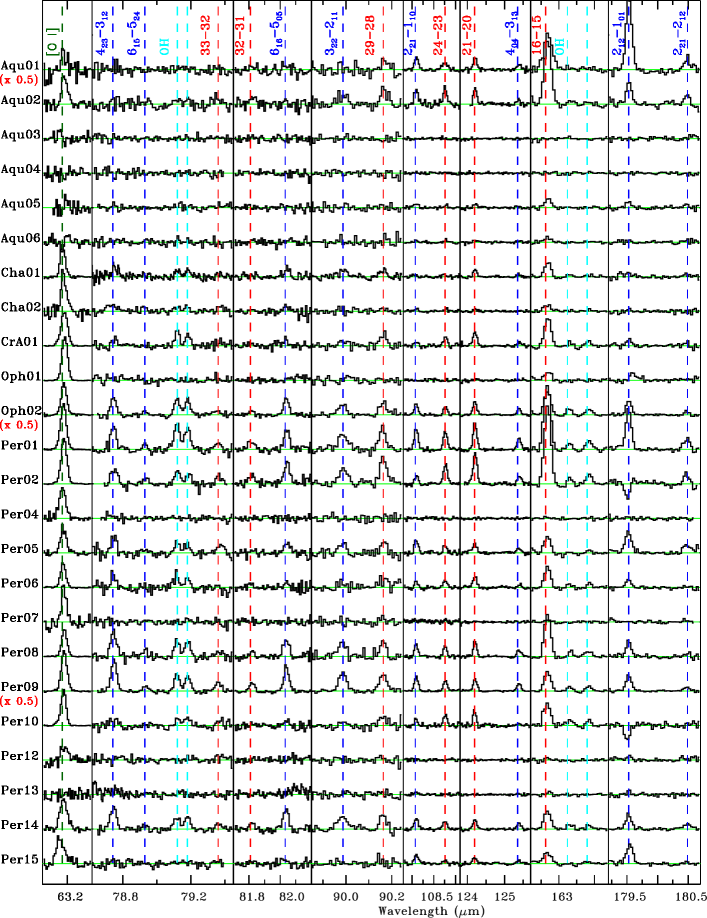
Figure 4: Overview of continuum-subtracted PACS spectra for selected lines. These are not corrected for the PSF. H₂O, CO and OH lines are marked in blue, red and cyan, respectively, with the [O i] marked in green. The y-axis of each spectrum for all lines except [O i] goes from 0 to 5 Jy, with the brightest sources scaled down by the factor indicated in red below the source name. The [O i] spectra are scaled separately by a factor between 0.05 and 1.

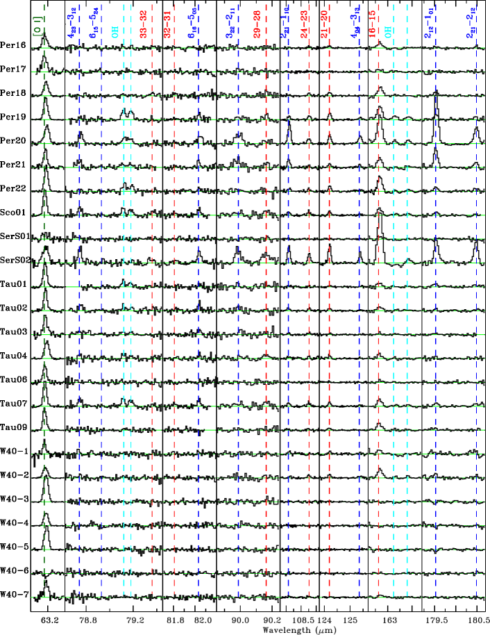
Figure 4 (Cont.): Overview of continuum-subtracted PACS spectra for selected lines. These are not corrected for the PSF. H₂O, CO and OH lines are marked in blue, red and cyan, respectively, with the [O i] marked in green. The y-axis of each spectrum for all lines except [O i] goes from 0 to 5 Jy, with the brightest sources scaled down by the factor indicated in red below the source name. The [O i] spectra are scaled separately by a factor between 0.05 and 1.

An overview of the PACS spectra for all sources is shown in Fig. 4, while an overview of the detection of all transitions is given in Table 14. An extensive analysis of the PACS data for WILL sources in the Perseus molecular cloud was published in Karska et al. (2014b), while a global study of PACS spectroscopy towards all WILL, DIGIT and WISH sources will be presented in Karska et al. (in prep.). Line flux densities were extracted from the PACS data as described in Karska et al. (2013).

The detection statistics for the main transitions are also given in Table 14. The most frequently detected line is [O i], which is detected in 42 out of 48 sources. Those sources not showing [O i] detections (AQU 03$-$06, PER 13 and W40 06) are generally not detected in other PACS lines. These sources have weak and/or narrow lines, where detected, in the HIFI observations (c.f. Fig. 2). There are 30 sources detected in at least one PACS water transition, while 27 are detected in at least one OH line and 32 in at least one CO line, with a detection more likely in the lower-energy transitions.

3.3 Ground-based follow-up

Follow-up ground-based observations were conducted towards the WILL sample, where not already available, to complement the Herschel spectral line information. Approximately half of the sources in the final catalogue were not part of the samples and regions already observed in HCO⁺ $J$=4$-$3 by Carney et al. (2016), so such observations were undertaken to confirm the embedded protostellar nature of the sample (see Appendix A.7). The follow-up observations also included maps of ¹²CO $J$=3$-$2 to characterise the entrained molecular outflow and C¹⁸O $J$=3$-$2 to obtain the source velocity and turbulent line-width in the cold envelope.

All but the two WILL sources in Chameleon are observable from the James Clerk Maxwell Telescope (JCMT) on Mauna Kea, Hawaii. Observations of C¹⁸O $J$=3$-$2 and HCO⁺ $J$=4$-$3 were obtained using HARP (Buckle et al., 2009) and the ACSIS autocorrelator at the JCMT as 2^′$\times$2^′ jiggle maps either as part of observing programs M12AN08 and M12BN07 or from the archive where these were already taken as part of other programs. These also included 2^′$\times$2^′ jiggle map observations of all sources in ¹²CO and H¹³CO⁺ $J$=4$-$3, while ¹³CO $J$=3$-$2 was obtained simultaneously with C¹⁸O $J$=3$-$2 for those sources that had not been previously observed. In a few cases, the ¹²CO and¹³CO observations were supplemented with cut-outs from the large basket-woven raster maps taken as part of the JCMT Gould Belt survey observations of Perseus, Taurus and Ophiuchus (Curtis et al., 2010; Davis et al., 2010; White et al., 2015).

For the two Chameleon sources, a series of lines were observed with the Atacama Pathfinder EXperiment (APEX) telescope at Llano de Chajnantor, Chile as part of project M0002_90. These consisted of 2^′$\times$2^′ on-the-fly maps of ¹²CO $J$=3$-$2 and 2$-$1, as well as single pointings of ¹²CO $J$=4$-$3, ¹³CO, C¹⁸O and C¹⁷O $J$=3$-$2 and 2$-$1, and HCO⁺ and H¹³CO⁺ $J$=4$-$3, using the FLASH⁺ (for the 300 GHz and 450 GHz bands) and APEX1 (for the 225 GHz band, Vassilev et al., 2008) receivers.

The initial reduction of the JCMT jiggle maps was performed using the most up-to-date version of the starlink reduction package orac-dr (Jenness et al., 2015). Similar initial reduction was performed for the APEX data using gildas-class. Following this, all data were (re-)baselined, corrected to the $T_{\mathrm{mb}}$ scale, and re-sampled to a common velocity scale with 0.2 km s^-1 resolution using customised python scripts. A summary of the observed lines, adopted beam efficiencies and typical $\sigma_{\mathrm{rms}}$ values obtained is presented in Table 19. ¹²CO emission is detected towards all sources but not all show evidence of outflows (see Sect. 4.1 and A.4 for more details). More details of detections and non-detections in the ¹³CO, C¹⁸O, C¹⁷O, HCO⁺ and H¹³CO⁺ spectra can be found in Sect. A.6.

4 Outflow characteristics and energetics

In this section we present selected characterisation and comparative analysis of the Herschel and ground-based spectral line observations, focusing on the entrained outflow as probed by ¹²CO $J$=3$-$2 and outflow/wind/jet-related shocks traced by PACS [O i] observations and the broader components of the HIFI H₂O and ¹²CO $J$=10$-$9 lines. In this and the following section, the pre-stellar and Class II sources are excluded from all analyses as they do not show strong outflow or envelope signatures (see Sect. A.7 for characterisation of sources).

Details of how the various entrained outflow-related properties (i.e. mass, momentum, energy, force and mass-loss rate, maximum velocity, dynamical time, inclination and radius) were measured are given in Appendix A.4, along with a table of their values for all WILL sources with detected outflows (Table 16). For consistency, the calculations are performed following the same method as that used by Yıldız et al. (2015) for the WISH sources, thus ensuring consistency between the WISH and WILL measurements.

4.1 Low-$J$ CO emission

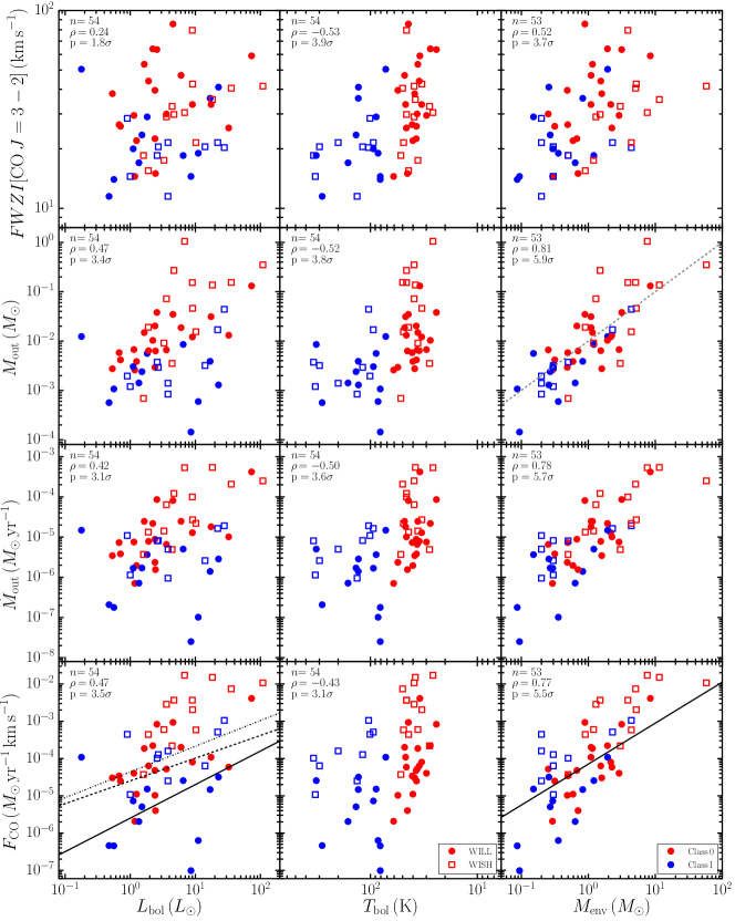
Figure 5: Comparison of FWZI, $M_{\mathrm{out}}$, $\dot{M}_{\mathrm{out}}$ and $F_{\mathrm{CO}}$ obtained from CO $J$=3$-$2 maps with $L_{\mathrm{bol}}$, $T_{\mathrm{bol}}$ and $M_{\mathrm{env}}$ for the WILL (filled symbols) and WISH (open symbols) sources. The number of sources, correlation coefficient and probability that the correlation is not simply due to random distributions in the variables are shown in the upper-left of each panel. The grey dashed line in the panel for $M_{\mathrm{out}}$ vs. $M_{\mathrm{env}}$ indicates where $M_{\mathrm{out}}/M_{\mathrm{env}}$=1$\%$. The solid black lines show the relations found by Bontemps et al. (1996) between $F_{\mathrm{CO}}$, $L_{\mathrm{bol}}$ and $M_{\mathrm{env}}$ for a sample of Class I sources. The dot-dashed black line shows the best-fit found between $F_{\mathrm{CO}}$ and $L_{\mathrm{bol}}$ by Cabrit & Bertout (1992) for a sample of Class 0 sources, while the dashed black line shows an extension to the low-mass regime of the fit to a sample of massive young sources from Maud et al. (2015).

One simple, initial question to ask is whether or not the observations are consistent with the common assumption that all embedded protostars have outflows. Overall 34/37 (92$\%$) of the Class 0/I sources in the WILL sample show outflow emission associated with the source in CO $J$=3$-$2 (shown in Fig. 17). Two of the Class II sources (CHA 01 and TAU 03) also show outflow activity, which is discussed further in Appendix C. Of the three Class 0/I sources without detections, Per 12, a Class 0 source, shows indications in Spitzer images that the outflow is in the plane of the sky (see Fig. 19 in Tobin et al., 2015, and associated discussion). Cha 02, a Class I, is faint or not detected in most tracers, but is detected in [O i] with PACS. W40 01, a Class 0, is also not detected in most PACS lines but shows a faint broad blue-shifted line-wing in the HIFI spectra. Thus the lack of detection for these three sources is likely due to sensitivity, meaning our observations are consistent with the hypothesis that all Class 0/I sources drive a molecular outflow.

An important next step in understanding the mechanism and impact of outflows on star formation is to constrain how the properties of outflows are related to those of the protostar. Figure 5 shows comparisons of the full-width at zero intensity (FWZI), which is the sum of the maximum velocities in the red and blue outflow lobes, mass in the entrained outflow ($M_{\mathrm{out}}$), the mass entrainment rate in the outflow ($\dot{M}_{\mathrm{out}}$) and the time-averaged momentum or outflow force ($F_{\mathrm{CO}}$) measured from CO $J$=3$-$2 with $L_{\mathrm{bol}}$, $T_{\mathrm{bol}}$ and $M_{\mathrm{env}}$ for all WISH and WILL Class 0/I sources. $\dot{M}_{\mathrm{out}}$ and $F_{\mathrm{CO}}$, as calculated quantities, are corrected for the inclination (see Appendix A.4 for details), while we do not correct for inclination for directly measured quantities, such as FWZI and $M_{\mathrm{out}}$.

The strongest correlation (5.9$\sigma$) is between the outflow mass and envelope mass, perhaps unsurprisingly given that the outflow is entrained from the envelope, with $M_{\mathrm{out}}/M_{\mathrm{env}}$ centred around 1$\%$, as shown by the grey dashed line. A significant, though weaker, correlation is also found between outflow mass and luminosity (3.4$\sigma$), possibly due to the correlation between $L_{\mathrm{bol}}$ and $M_{\mathrm{env}}$ (see Fig. 1). Since the mass is also an important factor in the calculation of $\dot{M}_{\mathrm{out}}$ and $F_{\mathrm{CO}}$, it is not surprising that both also show significant (i.e. $\geq$3$\sigma$) correlations with $M_{\mathrm{env}}$ and $L_{\mathrm{bol}}$. In general, all parameters decrease between Class 0 and Class I, as reflected in the significant negative correlations with $T_{\mathrm{bol}}$ seen for FWZI, $M_{\mathrm{out}}$, $\dot{M}_{\mathrm{out}}$ and $F_{\mathrm{CO}}$ (3.9, 3.8, 3.6 and 3.1$\sigma$ respectively).

Correlations of $F_{\mathrm{CO}}$ with $L_{\mathrm{bol}}$ and $M_{\mathrm{env}}$ have been known for some time, including Cabrit & Bertout (1992) who found the relationship between $F_{\mathrm{CO}}$ and $L_{\mathrm{bol}}$ indicated by the dot-dashed line in Fig. 5 for a sample of Class 0 sources, and Bontemps et al. (1996) who found the relationships indicated by the solid lines for a sample of primarily Class I sources. These have subsequently been confirmed to hold when extended to the high-mass regime for a sample of young protostars in Cygnus-X by Duarte-Cabral et al. (2013) and for a sample of massive young stellar objects (MYSOs) and young H ii regions by Maud et al. (2015). The relationships seen between these variables in the combined WISH and WILL sample are steeper than that found by Cabrit & Bertout (1992) and Bontemps et al. (1996). This may be due to differences in the calculation method (van der Marel et al., 2013), or to the fact that the luminosities were likely overestimated and the $F_{\mathrm{CO}}$ values underestimated in these previous studies due to the larger beam and lower sensitivity of older observations.

At first glance, the lower right panel of Fig. 5 would seem to show a slight offset in the $F_{\mathrm{CO}}$ measurements between the WISH and WILL samples, suggesting that either there is a difference in the measurements or that they come from distinct populations. However, there is no distinct break between the WISH and WILL sources, or between Class 0 and I when considering $M_{\mathrm{env}}$ vs. $M_{\mathrm{out}}$ and $\dot{M}_{\mathrm{out}}$, so the WISH sources are merely the extreme upper end of a continuous distribution. The WISH Class 0 sources were all chosen to be strong outflow sources, and the $M_{\mathrm{out}}$ and $\dot{M}_{\mathrm{out}}$ panels of Fig. 5 suggest that they are more prominent due to a larger reservoir of material (i.e. larger $M_{\mathrm{env}}$), rather than faster outflows as they have similar or even lower FWZI than the WILL sources.

For the Class I sources, there is little difference between the WISH and WILL sources in FWZI or $M_{\mathrm{out}}$, but the WISH Class I sources tend to have smaller outflows (see Table 16 for WILL sources and Table 3 in Yıldız et al., 2015, for WISH sources) resulting in larger values for the WISH sources of $\dot{M}_{\mathrm{out}}$ and $F_{\mathrm{CO}}$. This could be because the WISH Class I sources are typically in smaller, more isolated clouds with shorter distances from the protostar to the cloud edge than the Class I sources in WILL.

Let us now consider the physical implications of the main correlations between outflow and source properties. The correlation between $F_{\mathrm{CO}}$ and (current) $M_{\mathrm{env}}$ is often interpreted as the result of an underlying link between envelope mass and the mass accretion rate ($\dot{M}_{\mathrm{acc}}$), which is itself related to the driving of the outflow (Bontemps et al., 1996; Duarte-Cabral et al., 2013). As the central source evolves, $M_{\mathrm{env}}$ and $\dot{M}_{\mathrm{acc}}$ decrease, leading naturally to the decrease in $F_{\mathrm{CO}}$ and other outflow-related properties between Class 0 and I sources. The comparatively tight relationship between $M_{\mathrm{out}}$ and $M_{\mathrm{env}}$ further supports this interpretation.

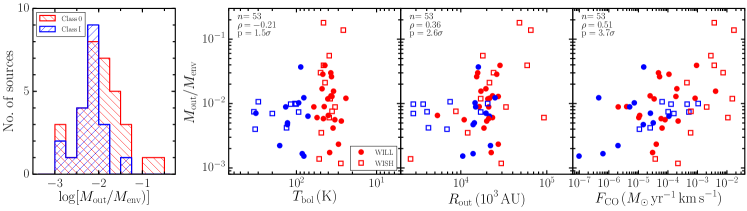
Figure 6: Histogram of the ratio of outflow to envelope mass (i.e. $M_{\mathrm{out}}$/$M_{\mathrm{env}}$) for Class 0 (red) and I (blue) sources (left), as well as how this varies with $T_{\mathrm{bol}}$ (middle-left), the mean length of the outflow lobes ($R_{\mathrm{out}}$, middle-right) and outflow force ($F_{\mathrm{CO}}$, right). The colours and symbols have the same meaning as in Fig. 5.

Indeed, the relation between $M_{\mathrm{out}}$ and $M_{\mathrm{env}}$ requires more investigation in its own right. Figure 6 shows a histogram of the fraction of mass in the outflow compared to the envelope (i.e. $M_{\mathrm{out}}$/$M_{\mathrm{env}}$), as well as how this varies with $T_{\mathrm{bol}}$ (as a more continuous proxy for source evolution), the mean length of the outflow lobes ($R_{\mathrm{out}}$), and the strength of the outflow as measured by $F_{\mathrm{CO}}$. The values of $M_{\mathrm{out}}$/$M_{\mathrm{env}}$ vary between $\sim$0.1 and 10$\%$, peaking around 1$\%$. The peak is similar between Class 0 and I with no significant trend with $T_{\mathrm{bol}}$, except that the Class 0 sources extend to larger values. This seems to be related to some Class 0 sources having longer outflows (i.e. larger $R_{\mathrm{out}}$) and thus have likely entrained additional material from the clump/cloud outside their original envelope. A statistically significant (3.7$\sigma$) correlation with $F_{\mathrm{CO}}$ is found, though with more than an order of magnitude spread.

The first impression of the peak value of $M_{\mathrm{out}}$/$M_{\mathrm{env}}$ being $\sim$10^-2 in the histogram shown in Figure 6 might be that this is rather low compared to a ‘typical’ star formation efficiency of 30$-$50$\%$ (e.g. Myers, 2008; Offner et al., 2014; Frank et al., 2014, and references therein). In order to understand whether or not this value is actually reasonable, let us first assume that the outflow is responsible for removing all of the envelope material that does not end up on the star. In this case, the average mass entrainment rate in the outflow over the Class 0+I lifetime ($\tau_{\mathrm{Class\,0/I}}$) is given by:

$$\dot{M}_{\mathrm{out}}\leavevmode\nobreak\ =\leavevmode\nobreak\ (1-\epsilon_{sf})\,\frac{M_{\mathrm{env}}}{\tau_{\mathrm{Class\,0+I}}}\,,$$ (3)

where $\epsilon_{sf}$ is the core-to-star formation efficiency, that is, the fraction of the envelope that will end up on the star. The observed mass-loss rate in the outflow, averaged along the flow, is given by:

$$M_{\mathrm{out}}\leavevmode\nobreak\ =\leavevmode\nobreak\ \dot{M}_{\mathrm{out}}\,t_{\mathrm{dyn}}\,,$$ (4)

where $t_{\mathrm{dyn}}$ is the dynamical time of the flow.

It is worth pointing out that $t_{\mathrm{dyn}}$ is not necessarily the age of the source, particularly if outflow activity is time-variable. Indeed, if ejection stops then, after some time, radiative losses and mixing with the ambient cloud material will dissipate all the angular momentum and energy from the flow, meaning that the observed $t_{\mathrm{dyn}}$ is likely a lower limit to the true ‘age’ of total accretion/outflow activity in a given source. However, if we assume that the overall mass outflow rate for a given burst is not significantly different from the average over the lifetime of the main accretion (i.e. Class 0+I) phase, or equally that protostellar outflows have an approximately constant entrainment efficiency per unit length, then we can combine and re-arrange Eqns. 3 and 4 to get:

$$\frac{M_{\mathrm{out}}}{M_{\mathrm{env}}}\leavevmode\nobreak\ =\leavevmode\nobreak\ (1-\epsilon_{sf})\frac{t_{\mathrm{dyn}}}{\tau_{\mathrm{Class\,0+I}}}\,.$$ (5)

The ratio of $t_{\mathrm{dyn}}$ to $\tau_{\mathrm{Class\,0+I}}$ effectively expresses the duty cycle of the outflow.

For $\tau_{\mathrm{Class\,0/I}}\approx$0.5 Myr (Dunham et al., 2015; Heiderman & Evans, 2015; Carney et al., 2016) and a typical dynamical time for the outflow of approximately 10⁴ yrs, the ratio of outflow to envelope mass has a value of $\sim$0.01 if the $\epsilon_{sf}$=0.5. Thus, while certainly missing some details, and being affected by variation from source to source and with time, the fact that we find median value for $M_{\mathrm{out}}/M_{\mathrm{env}}$ of approximately 1$\%$ is consistent with protostellar outflows having an approximately constant entrainment efficiency per unit length, a core-to-star formation efficiency of approximately 50$\%$, and an outflow duty cycle of order $\sim$5$\%$.

4.2 HIFI water and mid-$J$ CO emission

The water and CO $J$=10$-$9 spectra of many of the WILL sources show broad line wings, indicative of outflow emission, as seen in previous WISH observations (see e.g. Fig. 2 and Kristensen et al., 2012; San José-García et al., 2013; Mottram et al., 2014; San José-García et al., 2016). The FWZI of H₂O is strongly correlated with CO $J$=10$-$9 and $J$=3$-$2 (see Fig. 7), with H₂O consistently tracing faster material than these CO transitions, typically by a factor of $\sim$2. The narrower line-widths of CO $J$=10$-$9 with respect to CO $J$=3$-$2 are likely because the CO $J$=3$-$2 FWZI is calculated as the difference of the maximum red and blue velocity offsets anywhere in the 2^′$\times$2^′ maps while for CO $J$=10$-$9 this is measured from a single HIFI spectrum with a 18.4^′′ beam centred at the source position, that is, over a smaller region.

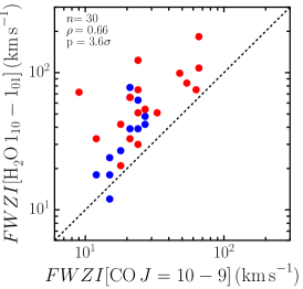
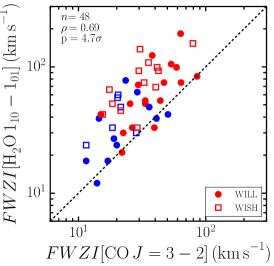
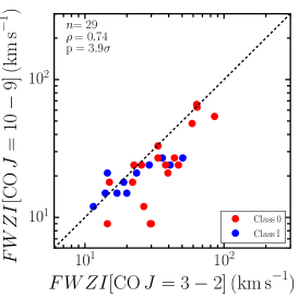
Figure 7: Comparison of the full-width at zero intensity widths of H₂O 1${}_{10}-$1₀₁, CO $J$=10$-$9 and 3$-$2. The dashed black lines indicate the line of equality.

Figure 8 shows a comparison of various source and outflow-related properties with the integrated intensity of the H₂O 1${}_{10}-$1₀₁ (557 GHz) line after scaling to a common distance of 200 pc. A linear scaling is used because the emission is dominated by outflows, which likely fill the beam along the outflow axis but not perpendicular to it (see Mottram et al., 2014, for more details). We are able to confirm the strong correlation found by Kristensen et al. (2012) for the WISH sample alone between the integrated intensity of the water line with its FWZI (at 6.0$\sigma$) and $M_{\mathrm{env}}$ (4.9$\sigma$). A new correlation is also found with $F_{\mathrm{CO}}$ (4.8$\sigma$), firmly showing that water emission is related to, though not tracing the same material as, the entrained molecular outflow. Furthermore, shallower trends of water line intensity with $L_{\mathrm{bol}}$ and inversely with $T_{\mathrm{bol}}$, hinted at but not significant in the WISH sample (e.g. see Fig. 6 of Kristensen et al., 2012), are now confirmed as statistically significant at 3.7 and 3.3$\sigma$ respectively.

To further examine the variation of water emission with source evolution, the lower-right panel of Fig. 8 shows the integrated intensity normalised by the source bolometric luminosity (thus minimising the contribution due to source brightness) vs. $M_{\mathrm{env}}/L_{\mathrm{bol}}^{0.6}$, which was proposed by Bontemps et al. (1996) as an evolutionary indicator. The clear positive correlation (4.1$\sigma$) seen in this panel reinforces the finding that the intensity of water emission decreases as sources evolve, independent of the relationship between integrated intensity and $L_{\mathrm{bol}}$.

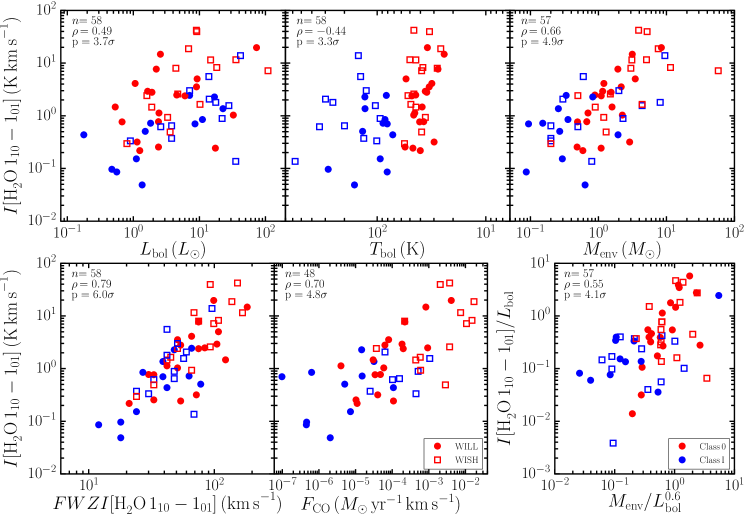
Figure 8: Comparison of the integrated intensity of H₂O 1${}_{10}-$1₀₁ linearly scaled to a distance of 200 pc with various source (top) and outflow-related (bottom left and middle) properties, as well as the integrated intensity normalised by $L_{\mathrm{bol}}$ vs. the evolutionary indicator $M_{\mathrm{env}}/L_{\mathrm{bol}}^{0.6}$ (bottom right) proposed by Bontemps et al. (1996). The number of sources, correlation coefficient and probability that the correlation is not just due to random distributions in the variables are shown in the upper-left of each panel.

The WILL observations therefore reinforce and confirm the results from WISH: H₂O traces a warmer and faster component of protostellar outflow than the cold entrained molecular outflowing material traced by low-$J$ CO (e.g. Nisini et al., 2010; Kristensen et al., 2012; Karska et al., 2013; Santangelo et al., 2013; Busquet et al., 2014; Mottram et al., 2014; San José-García et al., 2016). In addition, they confirm that the intensity of H₂O is related to envelope mass and the strength of the entrained molecular outflow, and is higher for younger and/or more luminous sources.

4.3 [O i] emission

It has been suggested for some time that emission from [O i] is a good alternative tracer of the mass loss from protostellar systems (e.g. Hollenbach, 1985; Giannini et al., 2001). In Class 0/I protostars it is thought to primarily trace the atomic/ionised wind, because most PACS observations are spectrally unresolved and those few sources that do show velocity-resolved emission (e.g. see Nisini et al., 2015) are dominated by the unresolved ($\lesssim$100 km s^-1) component. While there may be a contribution on-source from the disk, as in more evolved sources (see e.g Howard et al., 2013), [O i] emission in Class 0/I sources is often spatially extended and only fainter off-source by a factor of $\sim$2 compared to the peak position, so the wind likely still dominates.

The first comprehensive surveys of the [O i] 63 $\mu$m transition towards samples of YSOs, observed in an 80^′′ beam with the Infrared Space Observatory Long Wavelength Spectrometer (ISO-LWS Swinyard et al., 1998), suggested a link between the mass loss in [O i] and that in CO for Class 0 sources (Giannini et al., 2001). Only a marginal difference was seen in [O i] luminosity between Class 0 and I sources (Nisini et al., 2002), in contrast to the trend in CO. More recent studies by Podio et al. (2012) and Watson et al. (2016) with PACS on Herschel at 9^′′ resolution have used [O i] observations to claim trends of decreasing mass loss in the wind between Classes 0, I and II. However, both suffered from low number statistics, and Podio et al. (2012) mixed the same ISO results where no trend was found with early detections from Herschel PACS, which have significantly different beam sizes and observing methods that could induce such changes. For example, the chopping as part of PACS observations can cancel out up to 80$\%$ of the large-scale emission that is still detected by ISO (see Appendix E of Karska et al., 2013). The combined WILL, WISH and DIGIT dataset, with consistent observations of a large number of YSOs is ideally placed to help solve this issue.

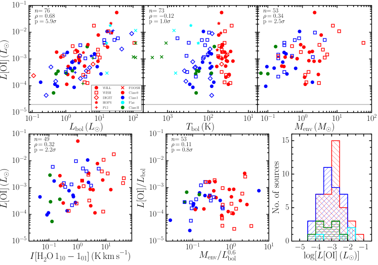
Figure 9: [O i] luminosity vs. $L_{\mathrm{bol}}$ (top-left), $T_{\mathrm{bol}}$ (top-middle), $M_{\mathrm{env}}$ (top-right) and integrated intensity in the H₂O 1${}_{10}-$1₀₁ transition (bottom-left). Bottom-middle: [O i] luminosity normalised by $L_{\mathrm{bol}}$ vs. the evolutionary indicator $M_{\mathrm{env}}/L_{\mathrm{bol}}^{0.6}$ proposed by Bontemps et al. (1996). The plots include data from the WILL, WISH and DIGIT samples, as well as from the literature from Podio et al. (2012) and the HOPS (Watson et al., 2016) and FOOSH (Green et al., 2013b) surveys where available. The number of sources and correlation statistics in the upper-right of each panel include only Class 0/I sources so as to be conservative. The horizontal grey line in the top panels indicates the upper limit for disk emission from Howard et al. (2013). Bottom-right: Histogram of $L$[O i] as a function of spectral type, including sources from all surveys.

Figure 9 shows the distribution of [O i] luminosity in the 63 $\mu$m line, integrated over the PACS spaxels associated with source outflows, and how this varies with various source parameters for the WILL, WISH and DIGIT samples (see Table 18 for $L$[O i] values). Also shown are the measurements from Herschel studies of a number of Class I/II sources in Taurus (Podio et al., 2012), the “Herschel Orion Protostars” survey (HOPS Watson et al., 2016), and the “FU Orionis Objects Surveyed with Herschel” survey (FOOSH Green et al., 2013b) which targeted a number of Flat spectrum and Class II sources that show evidence of FU Ori-type luminosity outbursts. None of the detected sources have a line luminosity below the upper limit for disk sources found by Howard et al. (2013) towards sources in Taurus (4$\times$10¹⁷ Wm^-2, corresponding to $\sim$2$\times$10^-5$L_{\odot}$ assuming a distance of 140 pc).

Two primary results stand out from Fig. 9. First, $L$[O i] is strongly correlated with $L_{\mathrm{bol}}$ but not with $M_{\mathrm{env}}$, with sources of all evolutionary classification following the overall trend. This is essentially the reverse of the situation found with low-$J$ CO, where the correlation is weak with $L_{\mathrm{bol}}$ and strong with $M_{\mathrm{env}}$ (see e.g. Fig. 5). H₂O shows clear correlations with both $M_{\mathrm{env}}$ and $L_{\mathrm{bol}}$ (see 8), though the relationship is slightly stronger with $M_{\mathrm{env}}$ than $L_{\mathrm{bol}}$, consistent with it tracing actively shocked outflow material between the entrained outflow, probed by low-$J$ CO, and the wind, probed by [O i].

Second, there is no statistically significant variation in $L$[O i] with evolutionary stage, either when considering the flat distribution between $L$[O i] and $T_{\mathrm{bol}}$ or the histogram of $L$[O i], which shows remarkably similar distributions for Class 0, I or II sources. This is not due to an evolutionary trend being masked by the correlation with $L_{\mathrm{bol}}$, as shown by the flat distribution in $L$[O i]$/L_{\mathrm{bol}}$ vs. $M_{\mathrm{env}}/L_{\mathrm{bol}}^{0.6}$. There is also no statistically significant correlation with envelope mass or integrated intensity in the H₂O 1${}_{10}-$1₀₁, which is dominated by the fast, actively shocked component of the molecular outflow.

This apparent contradiction between the evolutionary behaviour of mass-loss indicators, that is, the decrease of CO and H₂O velocity, intensity etc. as sources evolve compared to the invariance of [O i], will be explored and discussed in more detail in the following subsections. It is interesting to note that the FOOSH sources, which are all known to be undergoing luminosity outbursts, are on the upper end of, but consistent with, the distribution of other sources in terms of $L$[O i] vs. $L_{\mathrm{bol}}$. Thus, [O i] must react relatively quickly to variations in the mass accretion rate, which has a significant contribution to the observed source luminosity.

4.4 Mass accretion vs. loss

The balance of mass loss vs. accretion is important in revealing the rate at which the central protostar gains mass, as well as what fraction of the initial envelope will become part of the central source, that is, the core to star efficiency of star formation.

Direct measurement of the mass accretion rate is extremely challenging for embedded protostars because the UV, optical and near-IR continuum and lines typically used to do this in more evolved T-Tauri stars (e.g. Ingleby et al., 2013) are too heavily extincted. An approximate estimate can be obtained, however, by rearranging the equation for accretion luminosity, that is,

$$\dot{M}_{\mathrm{acc}}\leavevmode\nobreak\ =\leavevmode\nobreak\ \frac{L_{\mathrm{acc}}R_{*}}{GM_{*}}\,,$$ (6)

with the aid of a number of empirically constrained assumptions.

Firstly, accretion is assumed to generate all the observed bolometric luminosity for Class 0 sources and 50$\%$ for Class I sources, in keeping with the range observed in the few cases where this could be measured ($L_{\mathrm{acc}}$/$L_{\mathrm{bol}}$ = 0.1 $-$ 0.8: Nisini et al., 2005; Antoniucci et al., 2008; Caratti o Garatti et al., 2012). Next, a typical stellar mass ($M_{*}$) of 0.5$M_{\odot}$ for Class I sources is assumed and 0.2$M_{\odot}$ for Class 0 sources as they are still gaining mass, as in Nisini et al. (2015). The chosen values are for sources that will end up slightly more massive than the peak of the IMF ($\sim$0.2$M_{\odot}$, Chabrier, 2005). However, as already discussed in Section 2.2, our sample is biased towards slightly higher luminosities, and thus presumably stellar masses, than the global distribution, so this assumption is probably not far off. Indeed, these stellar masses are broadly in keeping with several recent mass determinations for similar embedded protostars from disk studies (Tobin et al., 2012; Murillo et al., 2013; Harsono et al., 2014; Codella et al., 2014). Finally, we assume a stellar radius ($R_{*}$) of 4$R_{\odot}$. The calculated values are given in Table 18 and shown vs. $L_{\mathrm{bol}}$, $T_{\mathrm{bol}}$ and $M_{\mathrm{env}}$ in the top panels of Fig. 10. The solid line in the upper-left panel shows the relation assumed in the evolutionary models of Duarte-Cabral et al. (2013), that is, Eqn. 2 with $\tau$=3$\times$10⁵ yrs.

Hollenbach (1985) noted a simple scaling between the [O i] line luminosity at 63 $\mu$m and the total mass-flux through the dissociative shock(s) producing it, given by:

$$\dot{M}_{\mathrm{s}}\leavevmode\nobreak\ =\leavevmode\nobreak\ 10^{-4}\leavevmode\nobreak\ L\mathrm{[O\mathsc{i}\,63\mu m]}\,.$$ (7)

For shocks generated by the wind, as is most likely the case for the emission probed by [O i], the mass flux through the shock(s), $\dot{M}_{\mathrm{s}}$, is related to the wind mass-flux, $\dot{M}_{\mathrm{w}}$, by the general formula (see Dougados et al., 2010):

$$\dot{M}_{\mathrm{s}}\leavevmode\nobreak\ =\leavevmode\nobreak\ N_{\mathrm{s}}\,\frac{\varv_{\mathrm{s}}}{\varv_{\mathrm{w}}\mathrm{cos}(\theta)}\dot{M}_{\mathrm{w}}\,,$$ (8)

where $N_{\mathrm{s}}$ is the number of shocks in the beam, $\varv_{\mathrm{s}}$ is the shock speed, and $\theta$ is the angle between the normal to the shock front and the wind direction (the 1/cos($\theta$) term then accounts for the ratio of the shock area to the wind cross section). It may be seen that $\dot{M}_{\mathrm{s}}$=$\dot{M}_{\mathrm{w}}$ in the simple case considered by Hollenbach (1985) if we are observing a static terminal shock where the wind is stopped against a much denser ambient medium; in this case, $N_{\mathrm{s}}$=1 and $\varv_{\mathrm{s}}$=$\varv_{\mathrm{w}}$cos($\theta$). This remains valid if the wind is not isotropic but collimated into a jet.

If we are instead observing weaker internal shocks travelling along the jet/wind, then $\varv_{\mathrm{s}}$$<<\varv_{\mathrm{w}}$cos($\theta$) but this will tend to be compensated for by the presence of several shocks in the beam (i.e. $N_{\mathrm{s}}>$1), as suggested by the chains of closely spaced internal knots seen in optical jets.

An alternative method for obtaining the average $\dot{M}_{\mathrm{w}}$ in this case is to consider that the [O i] emission is approximately uniform along the flow within the aperture, and to divide the emitting gas mass by the aperture crossing time. The derivation of emitting mass requires assumptions on the temperature and electron density, which are somewhat uncertain without also having observations of the [O i] 145 $\mu$m transition. However, Nisini et al. (2015) found that the differences are small between this alternative per-unit-length calculation and the Hollenbach (1985) formulation for a terminal static wind shock (i.e. $\dot{M}_{\mathrm{s}}$=$\dot{M}_{\mathrm{w}}$). Hence, although we note that there are some uncertainties involved, we adopt $\dot{M}_{\mathrm{w}}$[O i]=$\dot{M}_{\mathrm{s}}$ as given by Eqn. 7 to estimate the wind mass-flux from $L\mathrm{[O\mathsc{i}]}$ for our targets. The calculated values are given in Table 18.

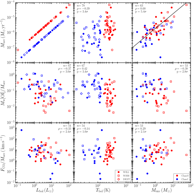
Figure 10: Mass accretion rate ($\dot{M}_{\mathrm{acc}}$, top), the ratio of mass-loss rate in the wind from [O i] to mass accretion rate (middle), and the ratio of outflow force from CO $J$=3$-$2 to mass accretion rate (bottom), vs. $L_{\mathrm{bol}}$ (left), $T_{\mathrm{bol}}$ (middle) and $M_{\mathrm{env}}$ (right). The solid line in the upper-right panel indicates the relationship between $\dot{M}_{\mathrm{acc}}$ and $M_{\mathrm{env}}$ from Duarte-Cabral et al. (2013), which is part of the evolutionary models shown in Fig. 1

The ratio of the mass-loss rate in the wind as measured from [O i] using Eqn. 7 to the mass accretion rate (i.e. $\dot{M}_{\mathrm{w}}$[O i]/$\dot{M}_{\mathrm{acc}}$) is compared to $L_{\mathrm{bol}}$, $T_{\mathrm{bol}}$ and $M_{\mathrm{env}}$ in the middle panels of Fig. 10. $\dot{M}_{\mathrm{w}}$[O i]/$\dot{M}_{\mathrm{acc}}$ varies from approximately 0.1$\%$ to 100$\%$ with a median of 13$\%$, in agreement with previous determinations (e.g. Cabrit, 2009; Ellerbroek et al., 2013) and in line with theoretical predictions (e.g. Konigl & Pudritz, 2000; Ferreira et al., 2006). However, approximately two-thirds of all Class 0 sources lie below 10$\%$.

The lower panels of Fig. 10 show similar comparison using the outflow force as measured from CO $J$=3$-$2. Assuming the entrainment process is momentum conserving:

$$F_{\mathrm{CO}}=\dot{M}_{\mathrm{w}}\,\varv_{\mathrm{w}}\epsilon_{\mathrm{ent}}\,,$$ (9)

where $\epsilon_{\mathrm{ent}}$ is the entrainment efficiency. The ratio with the mass accretion rate is then:

$$\frac{F_{\mathrm{CO}}}{\dot{M}_{\mathrm{acc}}}=\frac{\dot{M}_{\mathrm{w}}}{\dot{M}_{\mathrm{acc}}}\,\varv_{\mathrm{w}}\epsilon_{\mathrm{ent}}\,.$$ (10)

$\frac{\dot{M}_{\mathrm{w}}}{\dot{M}_{\mathrm{acc}}}\,\varv_{\mathrm{w}}$ is expected to be approximately constant due to conservation of angular momentum, with a value close to the Keplerian velocity of the disk at the launching radius (Duarte-Cabral et al., 2013).

We find that $F_{\mathrm{CO}}/\dot{M}_{\mathrm{acc}}$ is relatively invariant with $L_{\mathrm{bol}}$, $T_{\mathrm{bol}}$ and $M_{\mathrm{env}}$, as shown by values of the Pearson coefficient $\rho$ consistent with 0 (i.e. $p<$3$\sigma$). Taken together, this suggests that the efficiency of entrainment, $\epsilon_{\mathrm{ent}}$, is not dependent on source properties. The Keplerian velocity for a disk around a 0.2 or 0.5$M_{\odot}$ source is approximately 10$-$20 km s^-1 at 1AU, which, for a median value of $F_{\mathrm{CO}}/\dot{M}_{\mathrm{acc}}$ of 6.3 km s^-1, suggests values for $\epsilon_{\mathrm{ent}}$ of approximately 0.3$-$0.6. If the wind is launched at larger radii then $\epsilon_{\mathrm{ent}}$ could be closer to 1.

$L$[O i] does not vary with $T_{\mathrm{bol}}$, $M_{\mathrm{env}}$ or evolutionary stage (see Sect. 4.3 and Fig. 9), so the increase of $\dot{M}_{\mathrm{w}}$[O i]/$\dot{M}_{\mathrm{acc}}$ between Class 0 and I with increasing $T_{\mathrm{bol}}$ and with decreasing $M_{\mathrm{env}}$ is caused by the decrease in $\dot{M}_{\mathrm{acc}}$ , while $\dot{M}_{\mathrm{w}}$[O i] remains relatively constant. In contrast, the invariance of $F_{\mathrm{CO}}/\dot{M}_{\mathrm{acc}}$ is caused by both $\dot{M}_{\mathrm{acc}}$ and $\dot{M}_{\mathrm{w}}$ decreasing with increasing $T_{\mathrm{bol}}$ and decreasing $M_{\mathrm{env}}$ (see the lower panels of Fig. 5 for variation of $F_{\mathrm{CO}}$ with $T_{\mathrm{bol}}$ and $M_{\mathrm{env}}$). The reason for the difference in behaviour between these two measures of the ratio of mass loss to mass accretion is discussed further in the following section.

4.5 On the difference between [O i] and CO

The difference in behaviour between the atomic component of the wind (as traced by [O i]) and the entrained molecular outflow (as traced by low-$J$ CO) might seem to be in contradiction with models where the wind is the driving agent of the outflow (see e.g. Arce et al., 2007). Indeed a direct comparison, shown in Fig. 11, suggests that either the wind and outflow are not linked, [O i] is under-estimating the mass loss rate in the wind or $F_{\mathrm{CO}}$ is overestimated. However, there are several factors relating to what component of the system each tracer probes that argue against rushing to such a conclusion.

Figure 11: Ratio of mass-loss rate in the wind from [O i] to the outflow force from CO $J$=3$-$2. The dashed line indicates the expected locus if both trace the mass-loss rate in the wind, $\varv_{\mathrm{w}}$=100 km s^-1 and $\epsilon_{\mathrm{ent}}$=0.5. Lower values of $\varv_{\mathrm{w}}$ and/or $\epsilon_{\mathrm{ent}}$ move this line to the left. The symbols and colours have the same meaning as in Fig. 10.

First, [O i] only traces the atomic component of the wind and/or jet. Jets in Class 0 protostars are known to have a significant molecular component, as identified from high-velocity features (detected in e.g. CO, SiO and/or H₂O, Bachiller et al., 1991; Tafalla et al., 2010; Kristensen et al., 2011) with typical mass-loss rates of approximately 10${}^{-7}-$10^-5$M_{\odot}$ yr^-1 (e.g. Santiago-García et al., 2009; Lee et al., 2010a). These are typically approximately ten times higher than measured from [O i], but the molecular jet component disappears in older sources. This suggests an evolution in composition from molecular to atomic/ionised (see Nisini et al., 2015, for a detailed discussion), most likely due to increasing temperature of the protostar and decreasing density, and thus shielding, in the jet. Such arguments also hold for any wide-angle wind that could be present and contributing to driving the entrained CO outflow. Therefore, while the mass-loss rate due to the wind as a whole will decrease as the source evolves, in line with the decrease in the average mass accretion rate, the mass loss in the atomic component may remain approximately constant due to the shift in the composition of the wind.

Next, the optical depth of the continuum at 63 $\mu$m is likely considerable in the inner envelope in Class 0 sources (see e.g. Kristensen et al., 2012), so the observed [O i] flux may be significantly lower than the ‘true’ emission. The continuum optical depth will decrease as the source evolves and $M_{\mathrm{env}}$ decreases, which may also act to counteract the evolution in the mass loss in the wind. However, such an effect should also cause the ratio of the 63 $\mu$m to 145 $\mu$m [O i] lines to vary with continuum optical depth of the source, and a wavelength-dependent deficit in CO and H₂O transitions. Neither is clearly seen in PACS observations (see e.g. Karska et al., 2013). This is therefore likely a minor effect dominating only for sight-lines directly towards the protostar through the disk.

Finally, there is increasing evidence that episodic or time-variable accretion is important in embedded protostars from the very earliest phases of their evolution (see Dunham et al., 2014; Audard et al., 2014, for recent reviews). Accretion variability provides a consistent explanation for very low luminosity objects (e.g. Dunham et al., 2006), the observed spread and trends in protostellar (e.g. Dunham et al., 2010) and outflow related (e.g. Duarte-Cabral et al., 2013) properties, and luminosity bursts, brighter by at least a factor of ten, have now been observed in at least two embedded sources (Caratti o Garatti et al., 2011; Fischer et al., 2012; Safron et al., 2015). Chains of high-velocity molecular knots or ‘bullets’ observed in Class 0 outflows and jets, with typical spacings of 1000$-$10000 AU between minor and major episodes, respectively (e.g. Santiago-García et al., 2009; Lee et al., 2015), past heating of CO₂ ice (e.g. Kim et al., 2012) and the difference between the expected and observed CO snow surface in a number of protostars (Visser et al., 2015; Jørgensen et al., 2015) also provide indirect evidence of outbursts.

The imprint of time-variable accretion will be different for the molecular outflow and atomic wind, leading to differences in their properties. The luminosity will react quickly to any changes in the accretion rate (Johnstone et al., 2013), and thus traces the current or instantaneous activity. Since [O i] is dominated by the wind, it traces material that is closely related to the current accretion state and thus is correlated with luminosity regardless of whether the source is in outburst (e.g. the FOOSH sources) or not (see Fig. 9).

In contrast, the entrained molecular outflow traced by low-$J$ CO, particularly when measured over the full extent of the outflow, is an average of the ejection activity over at least 10${}^{3}-$10⁵ yrs. Indeed, the highest intensity in the entrained outflow as traced by low-$J$ CO is usually offset from the central source. If these spots represent major ejections triggered by accretion bursts, then such episodes should have occurred approximately hundreds to thousands of years ago, leaving enough time for the luminosity and circumstellar material to cool back to pre-burst levels (e.g. Arce & Goodman, 2001; Arce et al., 2013). Thus, the mass loss in the molecular outflow is related to the time-averaged mass-accretion rate and may be dominated by any periods of high accretion/ejection during outbursts (see also e.g. Dunham et al., 2006; Lee et al., 2010b).

The decrease of $F_{\mathrm{CO}}$ between Class 0 and I (see Fig. 5) therefore shows that the average mass accretion rate decreases as sources evolve, as originally proposed by Bontemps et al. (1996). The combination of decreasing mass accretion rates and episodic accretion was shown by Duarte-Cabral et al. (2013) to be consistent with the observed relationships between, and spread of, $L_{\mathrm{bol}}$, $M_{\mathrm{env}}$ and $F_{\mathrm{CO}}$. In particular, variation of the mass-accretion rate on shorter timescales than the dynamical timescale of the outflow helps to explain why outflow properties are less correlated with $L_{\mathrm{bol}}$ than with $M_{\mathrm{env}}$ (see Fig. 5 and Section 4.1). Those sources that show particularly high outflow forces and/or peak emission close to the source position may therefore have recently finished such a burst, or have a higher duty cycle of outburst to quiescent accretion. Thus, the mass-loss rate in the wind from [O i] and in the outflow force measured by low-$J$ CO are not directly correlated because the relationship between the current and time-averaged mass-accretion rate will be different for each source based on a complex combination of the source age, properties and mass-accretion history.

Some combination of the effects discussed above therefore causes the observed lack of correlation between CO and [O i]. As such, [O i] is not necessarily a direct alternative to CO for tracing mass loss and/or entrainment due to the jet/wind/outflow system in protostars, in contradiction to the early findings of Giannini et al. (2001).

5 Envelope

5.1 HCO⁺ vs. H₂O

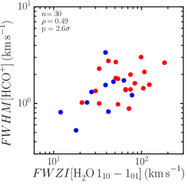
Figure 12: Comparison of the integrated intensity of HCO⁺ $J$=4$-$3 with $L_{\mathrm{bol}}$ (left) and the integrated intensity of H₂O 1${}_{10}-$1₀₁ scaled to a distance of 200 pc (middle), as well as the FWHM of HCO⁺ vs. the FWZI of H₂O 1${}_{10}-$1₀₁ (right). The number of sources, correlation coefficient and probability that the correlation is not just due to random distributions in the variables are shown in the upper-left of each panel.

Instead of outflows, HCO⁺ $J$=4$-$3 emission primarily traces cool, high-density envelope material ($T\sim$40 K, $n_{\mathrm{cr}}$=2$\times$10⁷ cm^-3 though the effective density for optically thick emission could be as low as 10⁴ cm^-3, see Shirley, 2015), and so is a relatively clean discriminator between young, embedded protostars and pre-stellar or more evolved disk sources (van Kempen et al., 2009; Carney et al., 2016). Spatially compact detections are found in this line towards most of the WILL sample sources, confirming them to be genuine embedded Class 0/I sources, while pre-stellar and Class II sources are either non-detections or show extended emission with no clear peak at the source position (see Appendix A.7 for details).

H₂O emission is a good tracer of warm, relatively dense material in shocks related to protostellar outflows ($T\gtrsim$300 K, $n$=10${}^{5}-$10⁸ cm^-3, Kristensen et al., 2013; Mottram et al., 2014). Sources with higher luminosities typically have stronger outflows (and thus stronger H₂O emission) and will lead, all other things being equal, to more mass at a given temperature in their envelopes and thus higher intensity in molecular tracers such as HCO⁺. It is therefore not unreasonable to expect that the emission in these two tracers may be related in Class 0/I sources.

Carney et al. (2016) compared the nature of HCO⁺ emission (compact, confused or extended/not detected) and the detection of water in the WILL PACS 179 $\mu$m observations. There are 18 sources in common between their sample and WILL: 13 are classified as Class 0/I (i.e. compact HCO⁺ $J$=4$-$3), 3 as confused and 2 as Class II (i.e. extended and/or non-detections in HCO⁺). Most sources (14/18) have detected 179 $\mu$m water emission, with four Class 0/I sources and one confused source showing extended emission. As both Class II sources were detected, while three Class 0/I sources and one confused source was not, Carney et al. (2016) did not find a clear relationship with evolution between the spatial distributions and detection of HCO⁺ and H₂O.

Considering the H₂O 1${}_{10}-$1₀₁ HIFI observations (see Fig. 12), for the two Class II sources, TAU 07 is not detected at the 3$\sigma$ level and TAU 09 shows very weak, narrow emission with an integrated intensity of 0.16 K km s^-1, equivalent to 10^-18 W m^-2, which could include a contribution from the disk (c.f. Podio et al., 2012, 2013; Fedele et al., 2013). Thus, while H₂O may be detected in either Class 0/I or II, the origin and intensity of the water emission changes as the source evolves. Strong detection of either HCO⁺ or water is therefore still a good indication of the youth of a protostar.

For the Class 0/I sources, the full WILL dataset enables the relationship between these species to be probed further by comparing the integrated intensity and FWHM of HCO⁺ with the integrated intensity and FWZI of the H₂O 1${}_{10}-$1₀₁ HIFI observations (see Fig. 12). HCO⁺ intensity is correlated both with $L_{\mathrm{bol}}$ and the intensity of the water line at 4.2 and 3.5$\sigma$ significance, respectively. There is not a strong, statistically significant relationship between the kinematics of the two lines and no significant line-wings are seen in the HCO⁺ spectra (see Fig. A.18). HCO⁺ $J$=4$-$3 therefore seems to primarily trace parts of the envelope that are further from, and thus less disturbed by, the outflow. HCO⁺ can be destroyed through reactions with H₂O (e.g. Jørgensen et al., 2013), so the higher abundance of H₂O in the outflow ($X[\mathrm{H}_{2}\mathrm{O}]$ or approximately 10${}^{-5}-$10^-7: Tafalla et al., 2013; Santangelo et al., 2013; Kristensen et al., subm.) compared to the envelope (10${}^{-8}-$10^-11: Mottram et al., 2013; Schmalzl et al., 2014) could be suppressing the HCO⁺ abundance in the outflow. This would explain why it is a poorer tracer of the outflow than might otherwise be expected. The correlation between the intensity of the two lines is therefore likely due to the relation between emission in each line and the source luminosity and structure, assisted by their tracing similar densities.

5.2 Infall signatures

The bulk of the H₂O emission comes from outflow-related shocks that have Gaussian-like profiles in velocity-resolved spectra. Once this contribution is removed, the residual profiles show the remaining water emission and/or absorption associated with the envelope. For the WISH sample, this process revealed seven sources with inverse P-Cygni line profiles indicative of infall and five with regular P-Cygni line profiles indicative of expansion motions in the envelope (Kristensen et al., 2012; Mottram et al., 2013). When the same procedure is performed for the WILL H₂O 1${}_{10}-$1₀₁ observations, removing the shock emission using the Gaussian decomposition of the profiles from San José-García (2015), six sources (3 Class 0 and 3 Class I) show inverse P-Cygni and two sources (both Class 0) show regular P-Cygni line profiles (see Fig. 13).

The two WILL sources in Serpens South have broad water absorption features, but they are not offset enough to be considered inverse P-Cygni (see Fig. 2). These may trace the large-scale cloud collision identified by Kirk et al. (2013), similar to that in the Serpens Main cloud first identified by Duarte-Cabral et al. (2011) and revealed to be the origin of the strong inverse P-Cygni line profile in water in Serpens-SMM4 by Mottram et al. (2013).

As an optically thick, higher density tracer, HCO⁺ $J$=4$-$3 is also sensitive to infall and expansion motions in protostellar envelopes (e.g. Gregersen et al., 1997; Myers et al., 2000). Though single-dish observations do not show absorption below the continuum, they can exhibit asymmetric line profiles, with the peak shifted to either the blue (infall) or red (expansion). The asymmetry between the red and blue peaks can be quantified using the $\delta\varv$ parameterisation suggested by Mardones et al. (1997, see Sect. A.6 for more details):

$$\delta\varv=\frac{\varv_{\mathrm{thick}}-\varv_{\mathrm{LSR}}}{\mathrm{FWHM}_{\mathrm{thin}}}\,,$$ (11)

where $\varv_{\mathrm{thick}}$ is the velocity of the peak emission in an optically thick tracer (in this case HCO⁺) and FWHM_thin is the line width of an optically thin tracer (in this case C¹⁸O). Values above or below 0.25 indicate a shift in the optically thick line of more than a quarter of the optically thin line width and so are considered significant. Thus, values above 0.25 indicate expansion motions while those below $-$0.25 indicate infall. Values between $-$0.25 and 0.25 are consistent with the optically thick and thin tracers being in agreement. A histogram of the values calculated for the WILL sample is shown in Fig. 14, with five sources showing blue asymmetry (i.e. $\delta\varv<-$0.25, 3 Class 0 and 2 Class I) and six showing red asymmetry (i.e. $\delta\varv>$0.25, 3 Class 0 and 3 Class I).

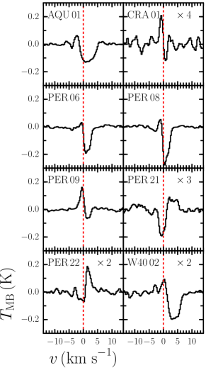
Figure 13: Outflow-subtracted H₂O 1${}_{10}-$1₀₁ residual line profiles for those sources showing either regular (PER 21 and PER 22) or inverse (all other) P-Cygni line profiles. All have been recentred so that the source velocity is at zero. The number in the upper-right corner of each panel indicates what factor the spectra have been multiplied by to aid visibility.

Figure 14: Histogram of the normalised offset of the peak of HCO⁺ 4$-$3 with respect to C¹⁸O 3$-$2. The red and blue dashed lines indicate the boundaries outside which the offset is considered significant (see Mardones et al., 1997).

Only one source (PER 08) exhibits non-static line signatures in both water and HCO⁺, however they conflict as the water shows an inverse P-Cygni line profile and the HCO⁺ a red asymmetry, leaving the status of this source uncertain. It is likely that these two tracers probe different radii, and so perhaps infall and expansion dominate in different parts of the envelope.

What is possibly more puzzling is that the vast majority of sources do not show indications of either infall or expansion in either tracer. Two-sample Kolmogorov-Smirnov (K-S) tests were performed comparing the cumulative distributions of source properties (e.g. $L_{\mathrm{bol}}$, $T_{\mathrm{bol}}$ etc.) for sources that show infall or expansion motions with respect to those that do not, in order to see if any source properties correlate with the detection of infall or expansion signatures. Only the integrated intensity of C¹⁸O 3$-$2 shows a statistically significant difference ($\leq$1$\%$ chance of being drawn from the same distribution) between sources with either an infall or expansion signature and those that do not: sources with higher C¹⁸O line intensity are more likely to show signs of infall.

Sources with clear infall motions are statistically more likely to have higher FWZI in ¹²CO 3$-$2, that is, broader outflow line-wings, than those showing no or expansion envelope motions (0.9$\%$ likelihood of coming from the same distribution). However, there are some sources that have high FWZI but no indication of radial envelope motions. One other result worth noting is that the presence of envelope motions is not more likely for certain values of outflow inclination (see van der Marel et al., 2013, and Sect. A.4 for details of how these were determined), suggesting that the orientation of the protostellar system is not the overriding cause of not detecting infall or expansion in our observations.

Infall must take place in all protostars, at least in the early phases, and at later times it seems unlikely that expansion of the envelope is restricted to a few select sources. Thus the low detection rate of such signatures in both tracers and the lack of a consistent trend with evolutionary Class is puzzling. It may well be that this is an observational effect, caused by small infall motions being lost in the general turbulent field on the large spatial scales that dominate single-dish observations. Mapping the velocity field inside protostellar envelopes with interferometers is likely needed to conclusively understand how material moves radially, and how this varies between different sources and over time (e.g. Yen et al., 2014; Aso et al., 2015; Evans et al., 2015).

6 Evolution of water line profile components from Class 0 to Class I

The intensity and line-width of water emission decreases for WISH sources between Class 0 and I (Kristensen et al., 2012; Mottram et al., 2014), while the rotational temperature of mid-$J$ CO and water excitation conditions do not (Karska et al., 2013; Mottram et al., 2014). Mottram et al. (2014) therefore suggested that the observed evolution in water line intensity and line-width from Class 0 to I was caused by a decrease in the velocity of the wind driving the outflow, due to the increase of the outflow cavity opening angle as proposed in the models of Panoglou et al. (2012), for example, rather than a decrease in density in the H₂O emitting gas. However, the small sample size of the WISH survey when broken down into evolutionary classifications meant that some trends, while hinted at by the data, were not statistically significant.

Inclusion of the WILL sample helps to resolve this issue. For example, Fig. 15 shows a histogram of the components found in HIFI water spectra, updated from that shown by Kristensen et al. (2012) to include the WILL survey sources and now using the more physically motivated nomenclature introduced by Mottram et al. (2014). A broad cavity shock component is observed in almost all Class 0 and I sources. Mottram et al. (2014) argued that this is caused by C-type shocks in the outflow cavity wall, though Yvart et al. (2016) suggest an alternate explanation where this component is formed in a dusty disk wind. Spot shock components, associated with offset J-type shocks either in bullets along the jet or at the base of the outflow (Kristensen et al., 2013; Mottram et al., 2014), are far more likely to be detected in Class 0 than Class I sources. Inverse P-Cygni line profiles associated with infall are more common for younger sources, though the inclusion of the WILL sample means that expansion motions traced by regular P-Cygni line profiles are now approximately equally common in both Class 0 and Class I sources. With the exception of the regular P-Cygni profiles, the evolution of water line profile components found for the combined WISH and WILL samples confirms the conclusion of Kristensen et al. (2012) and Mottram et al. (2014) that the outflows of young Class 0 sources are more energetic and their envelopes more infall-dominated than their more evolved Class I counterparts.

Figure 15: Bar chart of the number of shock and inverse/regular P-Cygni envelope components seen in water in the WISH (solid) and WILL (hatched) surveys for Class 0 (red) and I (blue) sources. The horizontal red and blue lines indicate the total number of Class 0 and I sources across both samples respectively.

Two-sample K-S tests show that there is less than 2$\%$ chance of the Class 0 and I distributions of $M_{\mathrm{env}}$, $M_{\mathrm{out}}$, $F_{\mathrm{CO}}$, $\dot{M}_{\mathrm{out}}$, the integrated intensity of HCO⁺ and H₂O 1${}_{10}-$1₀₁, and the FWZI of CO $J$=3$-$2 and H₂O 1${}_{10}-$1₀₁ being drawn from the same distribution, with the values for Class 0 sources being larger on average than those of Class I sources. In particular, this confirms the decrease in $F_{\mathrm{CO}}$ and both the line-width and intensity of water emission with evolution of the central source, reinforcing the direct relation between water emission and outflow/shock activity.

One caveat is that the Class 0 and I sources in WISH and WILL sources are not evenly drawn from the sampled star-forming regions. For example, only Class I or II sources are included in the Taurus star-formation region, while many of the Class 0 sources are in Perseus, which is a much more active star-forming complex. The observed differences and trends between Class 0 and I may therefore be accentuated by environmental differences. However, all the evidence suggests that Class I sources have slower, less powerful outflows and show less sign of strong infall motions in their envelopes than Class 0 sources.

7 Summary and conclusions

This paper has presented a set of Herschel and ground-based follow-up observations, characterisation and initial analysis of a flux-limited sample of Class 0/I YSOs in the Gould Belt. From this comprehensive dataset, combined with observations from the WISH and DIGIT surveys, we are able to conclude that:

• Water line profiles are dominated by emission from the actively shocked regions in outflows, the activity of which decreases in strength (i.e. has lower intensity and FWZI, see Fig. 8) and has fewer J-type shocks (i.e. fewer spot-shock components, see Fig. 15) as sources evolve from Class 0 to I. We also confirm the decrease in the force of the cooler and slower entrained outflowing gas, measured from low-$J$ CO, as young embedded protostars evolve.

• The ratio of mass in the entrained outflow to envelope mass (i.e. $M_{\mathrm{out}}/M_{\mathrm{env}}$) remains relatively constant between Class 0 and I with a median of approximately 1$\%$, consistent with a core-to-star formation efficiency of approximately 50$\%$ and an outflow duty cycle of approximately 5$\%$.

• $F_{\mathrm{CO}}/\dot{M}_{\mathrm{acc}}$ is relatively constant with $L_{\mathrm{bol}}$, $T_{\mathrm{bol}}$ and $M_{\mathrm{env}}$, suggesting that the entrainment efficiency is constant and independent of the power and evolution of the driving source of the flow. The constant value of $F_{\mathrm{CO}}/\dot{M}_{\mathrm{acc}}$ implies a median velocity at the wind launching radius of 6.3 km s^-1. This in turn suggests an entrainment efficiency of approximately 30$-$60$\%$ if the wind is launched around 1AU, or close to 100$\%$ if it is launched at larger radii.

• $L$[O i] is strongly correlated with $L_{\mathrm{bol}}$ but not with $M_{\mathrm{env}}$, in contrast to low-$J$ CO, which is strongly correlated with $M_{\mathrm{env}}$ and more weakly related to $L_{\mathrm{bol}}$. This suggests that [O i] is more closely related to the current accretion activity while low-$J$ CO traces the average activity over timescales of approximately 10${}^{2}-$10⁴ yrs. H₂O is more strongly correlated with $L_{\mathrm{bol}}$ than $M_{\mathrm{env}}$, but with a smaller difference than for low-$J$ CO, consistent with it tracing actively shocked material between the wind and entrained outflow.

• $L$[O i] does not vary significantly between Class 0 and I, likely because the molecular to atomic ratio in the wind and jet decreases as the source evolves, as suggested by Nisini et al. (2015). This could be caused by increased temperature and decreased density (and thus shielding) in more evolved sources. [O i] is therefore a poor tracer of the time-averaged mass-loss rate, and thus a poor alternative to CO.

• Infall signatures are predominantly seen in Class 0 sources in both H₂O and HCO⁺ single-dish observations, but with little overlap in detections between the two tracers. However, infall signatures remain elusive in the majority of sources. Thus, while water is a good tracer of infall, it is by no means the universal tracer needed to understand how this proceeds in general.

• The conclusions drawn from the WISH sample hold and become more statistically robust when the combined WISH+WILL+DIGIT sample is analysed.

Further exploitation of these data and this sample can be found for the HIFI data in San José-García (2015) and will be presented for the PACS data in Karska et al., (in prep.). The use of PACS and HIFI in this way is cementing the unique legacy of Herschel on the energetics of star formation and the origin of water in the interstellar medium.

Appendix A Property determination

This section presents the various properties of the WILL sources, and details of how they were determined.

A.1 Spectral energy distributions

In constructing the spectral energy distributions (SEDs) of the WILL sources, the photometric flux densities from the near-IR to 24 $\mu$m from 2MASS (Skrutskie et al. 2006) and Spitzer have been collected, where detected, from the latest determinations by Dunham et al. (2015). Flux densities for detections at 450 and/or 850 $\mu$m with SCUBA on the JCMT were taken from the catalogue of Di Francesco et al. (2008), and the 1.3 mm detections with MAMBO on the IRAM 30m telescope by Maury et al. (2011) for Aquila, Serpens South and W40 were also included.

All WILL sources lie within the Herschel PACS and SPIRE photometric maps observed in parallel-mode at 70, 160, 250, 350 and 500 $\mu$m as part of the Herschel Gould Belt Survey, with many also within the smaller regions observed in PACS-only mode at 100 and 160 $\mu$m. Where both parallel and PACS-only mode observations are available at 160 $\mu$m we use the data taken in PACS-only mode, as these were observed with a slower scanning speed and thus are of better quality than those data taken in parallel with SPIRE observations. Processed and calibrated mosaics were downloaded from the Herschel Science Archive (HSA, see also the Herschel Gould Belt survey archive for further products). The observation identification numbers for these maps are given in Table B.15.

Aperture photometry was then performed using python routines from the astropy package to extract flux densities for all sources at all available wavelengths. The starting value for the source aperture, inner and outer sky radii for each source at each wavelength was set at 6, 10 and 12 pixels, typically corresponding to 6, 10 and 12 times the beam size. Rings at these radii were then overlaid on images of the data and the radii adjusted to best encompass each source and local background respectively, while excluding nearby sources. Aperture correction factors were calculated and applied for each combination of aperture and sky annuli using the relevant PACS and SPIRE point source function images.

In some cases, additional nearby sources are blended with the primary WILL source at longer wavelengths where the Herschel beam becomes large. For these sources, we specify the longest wavelength where the sources are reliably separated. The flux densities at longer wavelengths are then scaled down by the ratio of the flux densities in the reliable image between the aperture used for that wavelength and the aperture used for the longer wavelength data. For example, if a source is blended at 500 $\mu$m, then the flux density at that wavelength is scaled down by the ratio of the flux density at 350 $\mu$m to the flux density in the 350 $\mu$m image within the region defined by the aperture used for the 500 $\mu$m data.

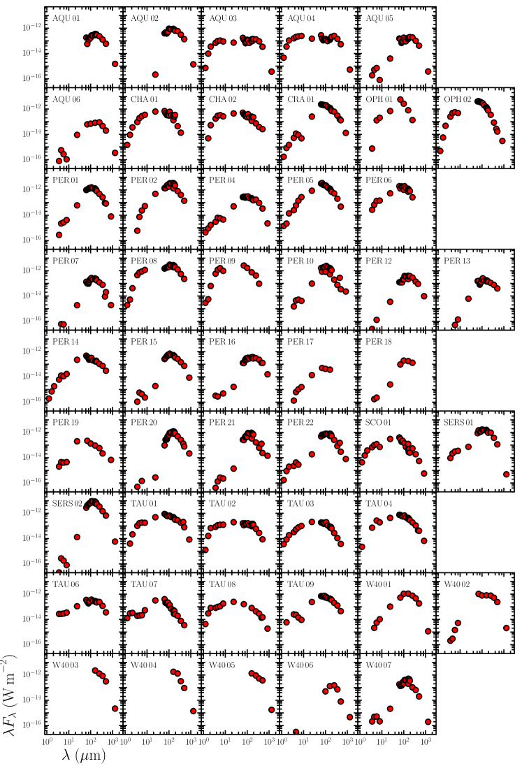
Figure 16: SEDs for all WILL sources. Data points from the PACS spectra are only included when used in the $L_{\mathrm{bol}}$ calculations.

Finally, continuum flux densities from the WILL PACS spectra were also obtained in the same manner as for the WISH sources (see Karska et al. 2013, for details). However, it is sometimes difficult in the PACS spectral maps to separate the emission related to the protostar from surrounding emission. Therefore, in cases where the PACS spectral continuum is significantly higher than obtained from the broad-band photometric maps, the latter is preferred and the PACS spectral continuum flux densities are not included in the SED. The broad-band photometric flux densities for all sources are given in Table 4, with the PACS spectral continuum flux densities given separately in Table 12. The SEDs of all sources are shown in Fig. 16.

For Aquila sources 01$-$04, the peak PACS continuum is offset from the coordinates in Maury et al. (2011), and so extraction of the SED and ground-based molecular line emission is performed at the peak flux position.

Table 4: SED photometric continuum fluxes. All numerical wavelengths in  $\mu$m.

Name	$J$	$H$	$K_{\mathrm{s}}$	3.6	4.5	5.8	8.0	24
	(mJy)	(mJy)	(mJy)	(mJy)	(mJy)	(mJy)	(mJy)	(mJy)
AQU 01	$-$	$-$	$-$	$-$	$-$	$-$	$-$	$-$
AQU 02	$-$	$-$	$-$	$-$	$-$	$-$	$-$	0001.72$\pm$0000.60
AQU 03	00.30$\pm$0.06	05.39$\pm$0.17	25.00$\pm$0.60	0083.40$\pm$004.17	0145.00$\pm$006.99	0205.00$\pm$009.76	0239.00$\pm$011.40	0581.00$\pm$0054.10
AQU 04	01.92$\pm$0.09	19.50$\pm$0.49	77.40$\pm$1.64	0190.00$\pm$009.28	0306.00$\pm$015.90	0441.00$\pm$020.80	0650.00$\pm$031.20	1190.00$\pm$0118.00
AQU 05	$-$	$-$	$-$	0000.22$\pm$000.02	0000.77$\pm$000.08	0001.37$\pm$000.09	0000.21$\pm$000.10	0031.90$\pm$0002.98
AQU 06	$-$	$-$	$-$	0000.09$\pm$000.01	0000.83$\pm$000.04	0000.52$\pm$000.06	0000.28$\pm$000.13	0072.60$\pm$0006.85
CHA 01	00.60$\pm$0.06	05.04$\pm$0.18	25.70$\pm$0.61	0112.00$\pm$010.10	0287.00$\pm$024.00	0533.00$\pm$027.00	0939.00$\pm$048.30	5080.00$\pm$0473.00
CHA 02	$-$	02.70$\pm$0.12	38.00$\pm$1.10	0210.00$\pm$010.00	0440.00$\pm$010.00	0640.00$\pm$031.00	0700.00$\pm$034.00	3600.00$\pm$0340.00
CRA 01	00.07$\pm$0.01	00.46$\pm$0.05	01.06$\pm$0.11	0006.30$\pm$000.71	0017.20$\pm$001.20	0017.30$\pm$001.10	0012.90$\pm$000.70	2040.00$\pm$0193.00
OPH 01	$-$	$-$	$-$	0000.90$\pm$000.25	$-$	0250.00$\pm$030.00	0550.00$\pm$130.00	5600.00$\pm$0840.00
OPH 02	00.20$\pm$0.04	03.10$\pm$0.28	34.00$\pm$2.10	0300.00$\pm$024.00	0730.00$\pm$048.00	1100.00$\pm$055.00	1300.00$\pm$065.00	$-$
PER 01	$-$	$-$	$-$	0000.33$\pm$000.04	0003.30$\pm$000.29	0005.20$\pm$000.36	0011.00$\pm$000.57	0480.00$\pm$0051.00
PER 02	$-$	$-$	$-$	0000.71$\pm$000.15	0011.00$\pm$000.74	0045.00$\pm$002.20	0140.00$\pm$007.10	3900.00$\pm$0420.00
PER 04	00.18$\pm$0.01	00.50$\pm$0.03	01.20$\pm$0.08	0003.60$\pm$000.29	0009.30$\pm$000.65	0011.00$\pm$000.77	0012.00$\pm$000.82	0400.00$\pm$0042.00
PER 05	00.58$\pm$0.03	01.20$\pm$0.15	10.00$\pm$0.50	0030.00$\pm$002.30	0089.00$\pm$005.70	0270.00$\pm$013.00	0720.00$\pm$041.00	6900.00$\pm$1200.00
PER 06	$-$	$-$	$-$	0032.00$\pm$002.20	0100.00$\pm$006.00	0260.00$\pm$013.00	0380.00$\pm$023.00	4300.00$\pm$0460.00
PER 07	$-$	$-$	$-$	$-$	0000.09$\pm$000.01	0000.11$\pm$000.03	$-$	0015.00$\pm$0001.60
PER 08	00.80$\pm$0.04	02.90$\pm$0.25	30.00$\pm$1.80	0540.00$\pm$046.00	1100.00$\pm$082.00	1700.00$\pm$210.00	3100.00$\pm$190.00	$-$
PER 09	01.20$\pm$0.06	03.10$\pm$0.29	45.00$\pm$2.80	0700.00$\pm$076.00	1800.00$\pm$170.00	3100.00$\pm$280.00	2600.00$\pm$250.00	$-$
PER 10	$-$	$-$	$-$	0001.80$\pm$000.18	0006.70$\pm$000.66	0010.00$\pm$000.83	0011.00$\pm$000.78	0770.00$\pm$0082.00
PER 12	$-$	$-$	$-$	0000.03$\pm$000.01	$-$	0000.25$\pm$000.04	$-$	0028.00$\pm$0003.00
PER 13	$-$	$-$	$-$	$-$	0000.02$\pm$000.01	0000.10$\pm$000.03	0000.37$\pm$000.04	0049.00$\pm$0005.20
PER 14	00.08$\pm$0.01	00.39$\pm$0.02	01.30$\pm$0.10	0007.30$\pm$000.53	0019.00$\pm$001.00	0022.00$\pm$001.10	0045.00$\pm$002.20	1800.00$\pm$0190.00
PER 15	$-$	$-$	$-$	0000.13$\pm$000.01	0000.85$\pm$000.07	0000.83$\pm$000.07	0000.62$\pm$000.06	0015.00$\pm$0001.50
PER 16	$-$	$-$	$-$	0000.39$\pm$000.08	0000.42$\pm$000.14	$-$	0001.30$\pm$000.11	0013.00$\pm$0001.40
PER 17	$-$	$-$	$-$	0000.16$\pm$000.01	0000.94$\pm$000.07	0002.00$\pm$000.15	0004.20$\pm$000.30	0110.00$\pm$0012.00
PER 18	$-$	$-$	$-$	$-$	0000.26$\pm$000.04	0000.44$\pm$000.05	$-$	0020.00$\pm$0002.10
PER 19	$-$	$-$	$-$	0002.40$\pm$000.17	0006.70$\pm$000.34	0007.90$\pm$000.40	0012.00$\pm$000.60	1600.00$\pm$0170.00
PER 20	$-$	$-$	$-$	0000.06$\pm$000.02	$-$	0000.28$\pm$000.06	$-$	0002.20$\pm$0000.34
PER 21	$-$	$-$	$-$	0000.05$\pm$000.01	0000.20$\pm$000.06	0000.52$\pm$000.06	0000.60$\pm$000.12	0011.00$\pm$0001.20
PER 22	00.07$\pm$0.01	00.49$\pm$0.03	01.40$\pm$0.16	0002.70$\pm$000.21	0006.30$\pm$000.66	0005.50$\pm$000.32	$-$	0150.00$\pm$0020.00
SCO 01	01.78$\pm$0.09	08.33$\pm$0.34	26.80$\pm$0.79	0081.80$\pm$004.33	0150.00$\pm$007.85	0231.00$\pm$010.90	0189.00$\pm$011.60	2430.00$\pm$0248.00
SERS 01	$-$	$-$	$-$	0011.30$\pm$000.56	0032.80$\pm$001.62	0060.20$\pm$002.84	0092.60$\pm$004.56	0582.00$\pm$0105.00
SERS 02	$-$	$-$	$-$	0000.02$\pm$000.01	0000.40$\pm$000.05	0000.35$\pm$000.06	0000.21$\pm$000.10	0105.00$\pm$0011.90
TAU 01	$-$	02.22$\pm$0.12	15.51$\pm$0.30	0121.49$\pm$005.59	0248.06$\pm$011.42	0350.51$\pm$016.14	0473.22$\pm$021.79	3887.74$\pm$0143.23
TAU 02	00.52$\pm$0.04	08.94$\pm$0.18	48.70$\pm$1.03	0101.99$\pm$004.70	0170.04$\pm$007.83	0238.07$\pm$010.96	0333.47$\pm$015.36	1576.52$\pm$0058.08
TAU 03	01.48$\pm$0.11	04.68$\pm$0.22	13.27$\pm$0.34	0038.42$\pm$001.77	0078.44$\pm$003.61	0147.47$\pm$006.79	0267.34$\pm$012.31	1666.00$\pm$0061.38
TAU 04	00.92$\pm$0.06	$-$	$-$	0087.21$\pm$004.02	$-$	0511.33$\pm$023.55	0514.12$\pm$023.68	3450.95$\pm$0128.24
TAU 06	$-$	$-$	$-$	0032.85$\pm$001.82	0041.17$\pm$001.90	0056.07$\pm$002.58	0092.70$\pm$004.27	0882.47$\pm$0032.51
TAU 07	05.14$\pm$0.16	16.50$\pm$0.46	23.44$\pm$0.54	0023.15$\pm$001.07	0030.38$\pm$001.40	0041.75$\pm$001.92	0141.54$\pm$006.06	2545.06$\pm$0093.76
TAU 08	01.77$\pm$0.07	16.50$\pm$0.53	58.55$\pm$1.19	0099.21$\pm$004.57	0146.74$\pm$006.76	0213.16$\pm$009.82	0477.60$\pm$021.99	1966.52$\pm$0072.44
TAU 09	$-$	03.27$\pm$0.19	$-$	0029.96$\pm$001.38	0034.88$\pm$001.61	0027.33$\pm$001.26	0024.61$\pm$001.13	1912.93$\pm$0070.47
W40 01	$-$	$-$	$-$	$-$	0003.19$\pm$000.18	0010.70$\pm$000.84	0027.40$\pm$003.78	0824.00$\pm$0078.40
W40 02	$-$	$-$	$-$	0000.25$\pm$000.09	0000.45$\pm$000.07	0002.80$\pm$001.01	0013.90$\pm$003.94	$-$
W40 03	$-$	$-$	$-$	$-$	$-$	$-$	$-$	$-$
W40 04	$-$	$-$	$-$	$-$	$-$	$-$	$-$	$-$
W40 05	$-$	$-$	$-$	$-$	$-$	$-$	$-$	$-$
W40 06	$-$	$-$	$-$	$-$	0000.05$\pm$000.01	$-$	$-$	$-$
W40 07	$-$	$-$	$-$	0000.25$\pm$000.03	0000.73$\pm$000.05	0001.00$\pm$000.07	0000.58$\pm$000.06	0017.00$\pm$0001.58

Table A.4 (Cont.): SED photometric continuum fluxes. All numerical wavelengths in  $\mu$m.

Name	70	100	160	250	350	450	500	850	1300
	(Jy)	(Jy)	(Jy)	(Jy)	(Jy)	(Jy)	(Jy)	(Jy)	(Jy)
AQU 01	001.33$\pm$0.03	005.89$\pm$0.08	015.07$\pm$0.25	019.43$\pm$0.67	014.85$\pm$0.69	$-$	009.87$\pm$0.52	$-$	000.65$\pm$0.26
AQU 02	010.88$\pm$0.20	030.77$\pm$0.35	047.80$\pm$1.01	049.43$\pm$1.23	036.19$\pm$1.12	$-$	022.82$\pm$0.79	$-$	000.60$\pm$0.19
AQU 03	002.84$\pm$0.06	004.09$\pm$0.05	007.08$\pm$0.14	010.94$\pm$0.41	010.75$\pm$0.60	$-$	005.69$\pm$0.48	$-$	000.16$\pm$0.06
AQU 04	003.56$\pm$0.09	004.72$\pm$0.07	006.67$\pm$0.17	020.56$\pm$0.52	016.71$\pm$0.66	$-$	008.98$\pm$0.77	$-$	000.23$\pm$0.10
AQU 05	003.21$\pm$0.08	005.95$\pm$0.08	009.45$\pm$0.19	015.47$\pm$0.49	011.88$\pm$0.83	$-$	006.98$\pm$0.60	$-$	000.16$\pm$0.06
AQU 06	001.44$\pm$0.06	002.32$\pm$0.06	004.38$\pm$0.24	007.44$\pm$0.62	005.33$\pm$0.62	$-$	003.30$\pm$0.50	$-$	000.15$\pm$0.06
CHA 01	010.87$\pm$0.23	010.23$\pm$0.14	006.99$\pm$0.17	003.67$\pm$0.25	001.58$\pm$0.26	$-$	$-$	$-$	$-$
CHA 02	008.87$\pm$0.17	007.48$\pm$0.10	006.25$\pm$0.13	006.11$\pm$0.43	004.42$\pm$0.54	$-$	004.29$\pm$0.47	$-$	$-$
CRA 01	051.72$\pm$0.94	064.45$\pm$0.65	066.03$\pm$0.81	051.78$\pm$0.89	035.52$\pm$0.77	023.84$\pm$4.77	021.79$\pm$0.51	003.68$\pm$0.74	$-$
OPH 01	134.00$\pm$1.60	088.39$\pm$0.78	043.25$\pm$1.18	011.22$\pm$1.48	$-$	$-$	$-$	$-$	$-$
OPH 02	098.24$\pm$1.82	103.55$\pm$1.18	071.39$\pm$1.14	029.44$\pm$0.96	009.99$\pm$0.76	004.11$\pm$0.82	002.78$\pm$0.51	000.85$\pm$0.17	$-$
PER 01	025.57$\pm$0.51	044.87$\pm$0.55	055.21$\pm$0.90	040.01$\pm$0.91	030.67$\pm$0.85	013.83$\pm$2.77	013.83$\pm$0.56	002.24$\pm$0.45	$-$
PER 02	032.16$\pm$0.72	060.76$\pm$0.97	070.74$\pm$2.59	067.82$\pm$2.70	047.30$\pm$2.46	$-$	023.14$\pm$1.44	$-$	$-$
PER 04	006.80$\pm$0.13	009.36$\pm$0.12	011.72$\pm$0.16	014.12$\pm$0.20	010.89$\pm$0.21	$-$	005.60$\pm$0.13	000.63$\pm$0.13	$-$
PER 05	081.94$\pm$1.59	077.36$\pm$0.92	066.27$\pm$1.03	044.23$\pm$0.76	023.63$\pm$0.61	$-$	007.93$\pm$0.35	$-$	$-$
PER 06	030.24$\pm$0.84	033.65$\pm$0.63	038.17$\pm$0.72	021.75$\pm$1.24	$-$	$-$	$-$	$-$	$-$
PER 07	002.30$\pm$0.05	007.75$\pm$0.13	011.47$\pm$0.26	010.05$\pm$0.32	009.05$\pm$0.43	001.38$\pm$0.28	003.38$\pm$0.36	000.54$\pm$0.11	$-$
PER 08	040.55$\pm$0.62	066.15$\pm$0.56	102.63$\pm$1.46	106.89$\pm$2.08	064.92$\pm$1.97	$-$	037.75$\pm$1.27	$-$	$-$
PER 09	060.37$\pm$2.08	055.78$\pm$1.24	040.46$\pm$1.89	034.99$\pm$2.77	011.04$\pm$1.34	$-$	$-$	$-$	$-$
PER 10	019.80$\pm$0.48	027.83$\pm$0.49	028.43$\pm$1.21	016.50$\pm$1.31	008.86$\pm$1.20	041.51$\pm$8.30	005.77$\pm$0.77	006.46$\pm$1.29	$-$
PER 12	002.87$\pm$0.07	006.96$\pm$0.13	011.60$\pm$0.32	023.94$\pm$0.60	016.26$\pm$1.09	013.63$\pm$2.73	$-$	002.74$\pm$0.55	$-$
PER 13	003.63$\pm$0.07	006.81$\pm$0.10	009.47$\pm$0.16	009.07$\pm$0.26	008.87$\pm$0.31	$-$	006.61$\pm$0.24	$-$	$-$
PER 14	008.76$\pm$0.17	008.65$\pm$0.11	009.73$\pm$0.13	008.88$\pm$0.22	008.65$\pm$0.29	$-$	005.08$\pm$0.21	$-$	$-$
PER 15	007.53$\pm$0.14	018.50$\pm$0.24	026.54$\pm$0.42	022.04$\pm$0.46	016.89$\pm$0.46	$-$	012.37$\pm$0.32	002.47$\pm$0.49	$-$
PER 16	002.90$\pm$0.06	008.34$\pm$0.11	019.21$\pm$0.30	025.29$\pm$0.52	026.48$\pm$0.64	019.55$\pm$3.91	020.97$\pm$0.48	004.53$\pm$0.91	$-$
PER 17	001.17$\pm$0.03	001.45$\pm$0.03	001.98$\pm$0.11	$-$	$-$	$-$	$-$	$-$	$-$
PER 18	002.24$\pm$0.05	006.44$\pm$0.09	009.50$\pm$0.24	010.88$\pm$0.65	$-$	$-$	$-$	$-$	$-$
PER 19	005.08$\pm$0.10	004.43$\pm$0.07	004.90$\pm$0.12	004.80$\pm$0.29	002.55$\pm$0.41	$-$	$-$	001.90$\pm$0.38	$-$
PER 20	006.18$\pm$0.13	021.36$\pm$0.27	042.63$\pm$0.76	041.10$\pm$1.49	030.42$\pm$1.35	019.88$\pm$3.98	012.88$\pm$0.77	006.13$\pm$1.23	$-$
PER 21	005.82$\pm$0.15	015.16$\pm$0.28	017.89$\pm$0.71	013.60$\pm$0.89	007.16$\pm$0.84	018.99$\pm$3.80	003.96$\pm$0.61	004.04$\pm$0.81	$-$
PER 22	015.46$\pm$0.31	026.24$\pm$0.40	028.13$\pm$0.83	021.27$\pm$0.80	009.88$\pm$0.62	022.52$\pm$4.50	004.96$\pm$0.36	002.24$\pm$0.45	$-$
SCO 01	007.16$\pm$0.15	$-$	006.57$\pm$0.11	004.52$\pm$0.15	002.21$\pm$0.15	$-$	000.92$\pm$0.11	000.16$\pm$0.03	$-$
SERS 01	034.27$\pm$0.49	056.60$\pm$0.36	084.69$\pm$0.73	080.67$\pm$1.28	043.57$\pm$1.30	$-$	019.09$\pm$0.92	$-$	000.21$\pm$0.05
SERS 02	096.64$\pm$1.39	219.00$\pm$1.75	327.90$\pm$4.45	283.98$\pm$8.56	172.40$\pm$6.58	$-$	109.94$\pm$3.96	$-$	002.50$\pm$0.31
TAU 01	018.67$\pm$0.38	$-$	024.18$\pm$0.29	023.52$\pm$0.39	020.99$\pm$0.43	030.74$\pm$6.15	013.20$\pm$0.31	002.38$\pm$0.48	$-$
TAU 02	002.67$\pm$0.05	$-$	005.09$\pm$0.06	004.92$\pm$0.20	003.28$\pm$0.23	$-$	001.46$\pm$0.16	$-$	$-$
TAU 03	004.21$\pm$0.09	$-$	004.77$\pm$0.09	002.27$\pm$0.13	001.27$\pm$0.13	$-$	000.63$\pm$0.09	$-$	$-$
TAU 04	017.04$\pm$0.37	$-$	018.77$\pm$0.33	015.82$\pm$0.32	012.66$\pm$0.36	006.62$\pm$1.32	006.86$\pm$0.24	001.87$\pm$0.37	$-$
TAU 06	005.96$\pm$0.12	$-$	014.23$\pm$0.13	020.28$\pm$0.28	013.72$\pm$0.32	$-$	006.05$\pm$0.21	$-$	$-$
TAU 07	004.77$\pm$0.09	004.10$\pm$0.05	002.88$\pm$0.06	001.60$\pm$0.10	000.89$\pm$0.15	$-$	000.59$\pm$0.13	$-$	$-$
TAU 08	003.76$\pm$0.08	$-$	004.28$\pm$0.07	003.59$\pm$0.14	003.35$\pm$0.17	002.05$\pm$0.41	002.47$\pm$0.14	000.53$\pm$0.11	$-$
TAU 09	015.73$\pm$0.26	018.11$\pm$0.17	023.20$\pm$0.24	017.00$\pm$0.36	014.60$\pm$0.43	$-$	007.46$\pm$0.46	$-$	$-$
W40 01	012.42$\pm$0.95	035.37$\pm$0.88	058.60$\pm$2.35	062.61$\pm$3.19	054.51$\pm$2.87	$-$	030.67$\pm$1.76	$-$	000.50$\pm$0.08
W40 02	024.33$\pm$3.36	026.28$\pm$1.73	042.81$\pm$2.71	063.53$\pm$3.16	060.78$\pm$2.87	$-$	039.55$\pm$1.80	$-$	000.90$\pm$0.24
W40 03	$-$	$-$	120.48$\pm$3.55	106.22$\pm$3.83	098.41$\pm$3.34	$-$	051.79$\pm$1.94	$-$	000.95$\pm$0.29
W40 04	$-$	$-$	095.75$\pm$3.06	108.24$\pm$3.46	037.51$\pm$3.02	$-$	015.47$\pm$1.72	$-$	000.60$\pm$0.14
W40 05	$-$	$-$	071.84$\pm$2.85	075.62$\pm$3.70	061.72$\pm$5.65	$-$	062.30$\pm$7.37	$-$	000.76$\pm$0.23
W40 06	$-$	001.68$\pm$0.09	007.01$\pm$0.40	012.62$\pm$0.91	008.58$\pm$0.85	$-$	001.33$\pm$0.77	$-$	000.20$\pm$0.06
W40 07	003.18$\pm$0.07	007.01$\pm$0.10	010.72$\pm$0.28	008.76$\pm$0.53	007.58$\pm$0.95	$-$	003.35$\pm$0.49	$-$	000.09$\pm$0.03

Table A.5: Pacs spectral continuum fluxes. All fluxes are given in Jy, all numerical wavelengths in  $\mu$m.

Name	63.2	79.2	81.8	84.6	90.0	108.8	125.4	157.7	164.0	169.1	179.5	190.0
AQU 01	003.8	004.5	003.8	003.6	005.5	009.7	011.3	018.5	018.2	017.5	020.4	018.5
AQU 02	008.4	010.1	012.2	013.1	015.1	031.3	034.9	046.5	046.6	044.4	046.3	039.9
AQU 03	003.7	002.5	002.2	001.8	002.4	003.8	002.9	004.8	006.2	005.4	008.5	008.6
AQU 04	005.8	002.9	003.6	003.9	004.0	004.1	004.0	006.4	007.4	008.6	010.5	013.2
AQU 05	003.2	001.8	002.3	002.2	002.7	004.3	003.9	007.2	008.7	009.1	011.2	012.7
AQU 06
CHA 01	014.7	009.7	009.0	010.2	011.2	022.0	013.8	016.6	016.6	015.8	015.4	021.7
CHA 02	010.9	009.4	008.3	007.6	009.3	014.3	009.3	013.0	013.6	013.8	013.8	014.5
CRA 01	049.4	057.7	056.9	058.4	062.5	071.5	062.9	065.2	060.7	055.9	054.5	045.5
OPH 01	139.1	157.8	161.3	161.5	159.7	161.0	137.4	111.0	102.6	094.0	086.7	073.4
OPH 02	084.7	098.7	099.3	102.2	101.9	102.5	084.6	075.8	069.4	064.3	059.1	049.1
PER 01	020.7	031.7	035.3	038.0	042.8	057.7	058.1	068.6	065.9	062.4	060.4	050.2
PER 02	029.1	055.7	060.1	066.4	078.6	122.1	139.4	186.0	182.9	177.1	175.8	141.7
PER 04	005.7	007.1	006.7	008.4	008.4	011.1	009.5	011.6	011.1	010.1	010.6	009.6
PER 05	067.1	067.8	067.3	070.0	071.7	075.3	065.2	065.3	062.0	057.5	054.0	045.0
PER 06	041.4	050.2	048.9	048.1	049.3	071.2	059.3	065.1	062.0	056.6	056.5	051.2
PER 07	002.8	002.5	003.2	004.0	005.7	009.7	009.0	013.1	013.1	011.9	013.2	010.9
PER 08	031.2	047.0	051.0	055.2	065.6	109.9	110.8	147.7	146.5	144.2	141.9	120.3
PER 09	242.5	291.1	301.7	308.8	324.4	398.7	357.1	310.7	281.6	260.8	227.9	190.6
PER 10	034.4	047.8	052.3	053.3	058.4	088.3	080.9	088.4	084.3	080.6	078.6	068.9
PER 12	002.6	003.6	003.3	003.4	006.1	014.1	014.6	021.0	020.8	020.5	022.8	024.0
PER 13	003.2	002.1	002.7	002.9	003.9	009.2	007.0	008.9	008.9	007.8	009.3	008.8
PER 14	009.9	009.0	007.3	006.5	007.9	011.4	008.5	009.1	010.0	009.3	011.3	010.0
PER 15	005.4	011.4	011.9	012.6	016.6	024.9	023.0	027.5	027.7	026.5	026.0	021.7
PER 16	002.7	005.1	006.4	006.4	008.9	011.8	011.9	018.6	019.5	018.3	022.5	018.2
PER 17	002.7	003.1	001.9	002.3	002.8	005.7	006.2	014.1	014.1	015.3	016.2	016.4
PER 18	003.0	005.1	005.3	005.5	008.1	011.5	012.0	020.3	019.6	020.0	020.4	020.5
PER 19	000.9	003.2	002.5	003.1	003.5	006.7	004.5	007.9	007.0	006.8	008.4	010.8
PER 20	002.0	007.3	009.5	011.9	015.6	033.9	043.2	065.0	066.8	063.6	064.6	054.3
PER 21	005.6	011.1	013.0	013.4	017.0	032.8	034.8	049.8	049.0	046.7	046.9	042.8
PER 22	010.3	015.8	018.2	019.2	021.5	029.2	031.5	040.9	043.5	040.8	041.2	032.7
SCO 01	008.4	004.9	005.0	005.9	006.5	005.0	002.9	002.8	002.3	001.5	002.8	001.6
SERS 01	018.4	028.6	029.9	032.6	035.7	059.8	063.9	077.5	074.9	072.2	070.8	060.4
SERS 02	058.8	134.4	148.5	163.4	193.3	327.2	370.8	452.4	440.3	425.2	411.8	333.8
TAU 01	018.8	017.4	017.4	017.0	018.2	023.6	021.4	026.4	025.5	024.1	023.7	019.9
TAU 02	003.4	004.4	003.8	003.6	004.4	005.9	004.7	007.6	006.6	007.0	008.8	007.7
TAU 03	003.9	004.5	004.8	004.1	005.2	007.0	004.6	004.6	004.0	004.5	004.8	004.0
TAU 04	015.9	016.9	016.6	017.0	017.1	024.2	019.9	022.7	023.0	021.1	019.7	018.3
TAU 06	007.4	004.9	005.8	006.5	007.8	013.4	012.2	014.6	015.3	013.7	015.7	014.1
TAU 07	008.4	004.9	005.0	005.9	006.5	005.0	002.9	002.8	002.3	001.5	002.8	001.6
TAU 08
TAU 09	014.7	017.3	019.5	019.9	022.0	022.0	020.4	023.3	022.8	022.6	023.1	021.7
W40 01	036.7	067.3	077.2	084.7	103.8	193.8	226.6	274.0	267.7	252.9	240.7	193.0
W40 02	537.6	455.5	454.6	446.9	431.4	400.4	324.3	267.7	247.2	230.2	209.5	180.1
W40 03	128.8	204.8	219.6	230.9	251.7	352.6	353.5	363.1	339.4	316.0	288.7	238.3
W40 04	208.7	303.3	323.7	340.3	372.4	496.3	465.4	429.8	395.4	363.5	324.5	268.3
W40 05	106.8	173.7	187.8	200.3	228.2	343.1	346.4	362.9	335.7	316.1	291.6	238.9
W40 06	$-$	$-$	$-$	$-$	$-$	$-$	$-$	$-$	$-$	000.1	006.3	008.5
W40 07	003.9	003.8	005.0	005.3	008.0	014.4	017.0	025.9	027.4	024.8	027.4	022.2

A.2 Continuum properties

A number of properties are often calculated from YSO SEDs in order to characterise them. While previous determinations have been made for the better-studied members of the WILL sample, variations in method and implementation could lead to biases or systematic effects between sources in different regions. In addition, Herschel data provide significantly higher-resolution images for flux density determination than were previously available between 70 and 250 $\mu$m (e.g. Herschel has a FWHM of $\sim$8^′′ at 100 $\mu$m compared to 3^′$\times$5^′ for IRAS). In order to be consistent with other Herschel surveys, most notably the WISH and DIGIT surveys, we follow the definitions in Dunham et al. (2010) and calculate the bolometric luminosity ($L_{\mathrm{bol}}$) using:

$$L_{\mathrm{bol}}\leavevmode\nobreak\ =\leavevmode\nobreak\ 4\pi d^{2}\int_{0}^{\infty}F_{\nu}\mathrm{d}\nu\,,$$ (12)

the sub-mm luminosity using:

$$L_{\mathrm{smm}}\leavevmode\nobreak\ =\leavevmode\nobreak\ 4\pi d^{2}\int_{0}^{\nu=c/350\mu\mathrm{m}}F_{\nu}\mathrm{d}\nu\,,$$ (13)

and bolometric temperature using:

$$T_{\mathrm{bol}}\leavevmode\nobreak\ =\leavevmode\nobreak\ 1.25\times 10^{-11}\frac{\int_{0}^{\infty}\nu F_{\nu}\mathrm{d}\nu}{\int_{0}^{\infty}F_{\nu}\mathrm{d}\nu}\,.$$ (14)

In these equations, $F_{\nu}$ is the flux density at frequency $\nu$, and $d$ is the distance to the source. The integrals were calculated over the available SED flux densities using trapezium integration, which was found by Karska et al. (2013) to provide the most consistent results for the WISH survey sources.

The infrared spectral index (see Lada 1987) is also calculated for those sources where the source is detected in at least three wavelengths between 2 and 25 $\mu$m using a least-squares linear fit to the logarithms of wavelength and flux density such that:

$$\alpha_{\mathrm{IR}}\leavevmode\nobreak\ =\leavevmode\nobreak\ \frac{d\,log_{10}(\lambda F_{\lambda})}{d\,log_{10}(\lambda)}\,,$$ (15)

where $F_{\lambda}$ is the flux density at wavelength $\lambda$.

Finally, for the sources in the Aquila Rift we take the envelope mass ($M_{\mathrm{env}}$) from Maury et al. (2011), calculated from the integrated intensity at 1.2 mm, corrected to the updated distance for that region. In other regions we calculate $M_{\mathrm{env}}$ for those sources with SCUBA 850 $\mu$m observations using Eqn. 1 from Jørgensen et al. (2009):

$$M_{\mathrm{env}}\,=\,0.44\,\left(\frac{L_{\mathrm{bol}}}{1\,L_{\odot}}\right)^{-0.36}\left(\frac{S_{15^{\prime\prime},\,850\mu\mathrm{m}}}{1\,\mathrm{Jy\,beam}^{-1}}\right)^{1.2}\left(\frac{d}{125\,\mathrm{pc}}\right)^{1.2}\leavevmode\nobreak\ M_{\odot}\,,$$ (16)

where $S_{15^{\prime\prime},\,850\mu\mathrm{m}}$ is the peak SCUBA 850 $\mu$m flux density in a 15^′′ pixel. This empirical relation was derived from comparison of observed source properties with the results of dust radiative transfer models. The results of these calculations are summarised in Table 1.

A.3 PACS line properties and detection statistics

Table A.6: Principle lines observed with PACS.

Species	Transition	Rest Frequency	Wavelength	Eu/$k_{\mathrm{b}}$	$A_{\mathrm{ul}}$	$n_{\mathrm{cr}}$	$\theta_{mb}$	Obs. Time
		(GHz)	( $\mu$m)	(K)	(s-1)	(cm-3)	(′′)	(min)
o-H2O	2${}_{12}-$101	1669.90477	179.527	0114.4	5.59$\times$10-2	3$\times$10${}^{8\phantom{0}}$	12.7	36
	2${}_{21}-$212	1661.00764	180.488	0194.1	3.06$\times$10-2	1$\times$10${}^{8\phantom{0}}$	12.8	36
	2${}_{21}-$110	2773.97659	108.073	0194.1	2.56$\times$10-1	1$\times$10${}^{9\phantom{0}}$	07.6	17
	4${}_{23}-$312	3807.25841	078.742	0432.2	4.84$\times$10-1	2$\times$10${}^{9\phantom{0}}$	05.6	36
	6${}_{16}-$505	3654.60328	082.031	0643.5	7.49$\times$10-1	4$\times$10${}^{9\phantom{0}}$	05.8	36
	7${}_{16}-$707	3536.66681	084.770	1013.2	2.16$\times$10-1	1$\times$10${}^{9\phantom{0}}$	06.0	36
	8${}_{18}-$707	4734.29617	063.323	1070.7	1.75$\times$10${}^{0\phantom{-}}$	1$\times$1010	04.5	17
p-H2O	3${}_{22}-$211	3331.45838	089.988	0296.8	3.52$\times$10-1	1$\times$10${}^{9\phantom{0}}$	06.4	36
	4${}_{04}-$313	2391.57263	125.354	0319.5	1.73$\times$10-1	9$\times$10${}^{8\phantom{0}}$	08.9	36
	6${}_{15}-$524	3798.28164	078.928	0781.1	4.52$\times$10-1	2$\times$10${}^{9\phantom{0}}$	05.6	36
OH	${}^{1}/_{2}$,${}^{1}/_{2}-^{3}/_{2}$,${}^{3}/_{2}$	3786.16998	079.181	0181.7	3.52$\times$10-2	1$\times$10${}^{8\phantom{0}}$	05.6	36
	${}^{1}/_{2}$,${}^{1}/_{2}-^{3}/_{2}$,${}^{3}/_{2}$	3789.17979	079.118	0181.9	3.49$\times$10-2	8$\times$10${}^{7\phantom{0}}$	05.6	36
	${}^{3}/_{2}$,${}^{1}/_{2}-^{1}/_{2}$,${}^{1}/_{2}$	1834.74735	163.397	0269.8	6.37$\times$10-2	2$\times$10${}^{8\phantom{0}}$	11.6	36
	${}^{3}/_{2}$,${}^{1}/_{2}-^{1}/_{2}$,${}^{1}/_{2}$	1837.81682	163.124	0270.2	6.40$\times$10-2	2$\times$10${}^{8\phantom{0}}$	11.5	36
	${}^{7}/_{2}$,${}^{3}/_{2}-^{5}/_{2}$,${}^{3}/_{2}$	3543.77937	084.597	0290.5	5.13$\times$10-1	2$\times$10${}^{9\phantom{0}}$	06.0	36
	${}^{7}/_{2}$,${}^{3}/_{2}-^{5}/_{2}$,${}^{3}/_{2}$	3551.18525	084.420	0291.2	5.16$\times$10-1	2$\times$10${}^{9\phantom{0}}$	06.0	36
[O i]	${}^{3}P_{1}-^{3}P_{2}$	4744.77749	063.184	0227.7	8.91$\times$10-5	5$\times$10${}^{5\phantom{0}}$	04.5	17
CO	16$-$15	1841.34551	162.812	0751.7	4.05$\times$10-4	1$\times$10${}^{6\phantom{0}}$	11.5	36
	21$-$20	2413.91711	124.193	1276.1	8.83$\times$10-4	2$\times$10${}^{6\phantom{0}}$	08.8	36
	24$-$23	2756.38758	108.763	1656.5	1.28$\times$10-3	3$\times$10${}^{6\phantom{0}}$	07.7	17
	29$-$28	3325.00528	090.163	2399.8	2.13$\times$10-3	6$\times$10${}^{6\phantom{0}}$	06.4	36
	31$-$30	3551.59236	084.411	2735.3	2.52$\times$10-3	7$\times$10${}^{6\phantom{0}}$	06.0	36
	32$-$31	3664.68418	081.806	2911.2	2.74$\times$10-3	7$\times$10${}^{6\phantom{0}}$	05.8	36
	33$-$32	3777.63573	079.360	3092.5	2.95$\times$10-3	8$\times$10${}^{6\phantom{0}}$	05.6	36
[C ii]	${}^{2}P_{{}^{3}/_{2}}-^{2}P_{{}^{1}/_{2}}$	1900.53690	157.741	0091.2	2.32$\times$10-6	3$\times$10${}^{3\phantom{0}}$	11.2	36

Table LABEL:T:observations_pacs_settings gives the wavelength ranges covered by the two PACS settings used for the WILL survey. Table LABEL:T:observations_pacs_lines summarises the properties of the principle transitions observed with PACS towards the WILL sample, while Table 14 indicates which of these are detected towards each WILL source. The overall fraction of sources detected in each transition is also given in the bottom row of Table 14. The spectral resolution of PACS is not sufficient to separate the CO $J$=31$-$30 transition at 84.41 $\mu$m and the OH 84.42 $\mu$m transition. Emission at this wavelength is therefore marked as a detection for both lines but could be in only CO or OH. The detection (or not) of neighbouring transitions is likely a reasonable estimate of whether the detected emission is from CO, OH or a blend of the two.

Table A.7: PACS line detections.

Name	o-H2O							p-H2O			[O i]
	$2_{12}-1_{01}$	$2_{21}-2_{12}$	$2_{21}-1_{10}$	$4_{23}-3_{12}$	$6_{16}-5_{05}$	$7_{16}-7_{07}$	$8_{18}-7_{07}$	$3_{22}-2_{11}$	$4_{04}-3_{13}$	$6_{15}-5_{24}$	${}^{3}P_{1}-^{3}P_{2}$
AQU 01	Y	Y	Y	N	N	N	N	N	Y	N	Y
AQU 02	Y	Y	Y	N	N	N	N	Y	Y	N	Y
AQU 03	N	N	N	N	N	N	N	N	N	N	N
AQU 04	N	N	N	N	N	N	N	N	N	N	N
AQU 05	Y	N	Y	N	N	N	N	N	N	N	N
AQU 06	N	N	N	N	N	N	N	N	N	N	N
CHA 01	Y	N	Y	Y	Y	N	N	Y	Y	N	Y
CHA 02	N	N	Y	Y	Y	N	N	N	N	Y	Y
CRA 01	Y	N	Y	Y	N	N	N	Y	Y	N	Y
OPH 01	Y	N	N	N	N	N	N	N	N	N	Y
OPH 02	Y	Y	Y	Y	Y	N	Y	Y	Y	Y	Y
PER 01	Y	Y	Y	Y	Y	N	Y	Y	Y	Y	Y
PER 02	Y	Y	Y	Y	Y	N	Y	Y	Y	Y	Y
PER 04	N	N	N	N	N	N	N	N	N	N	Y
PER 05	Y	Y	Y	Y	Y	N	N	Y	Y	Y	Y
PER 06	Y	N	Y	Y	Y	N	Y	N	Y	N	Y
PER 07	N	N	N	N	N	N	N	N	N	N	Y
PER 08	Y	N	Y	Y	Y	N	Y	Y	Y	N	Y
PER 09	Y	Y	Y	Y	Y	N	Y	Y	Y	Y	Y
PER 10	Y	N	Y	N	N	N	N	N	Y	N	Y
PER 12	N	N	N	N	N	N	N	N	N	N	Y
PER 13	N	N	Y	N	N	N	N	N	Y	N	N
PER 14	Y	Y	Y	Y	Y	N	Y	Y	Y	N	Y
PER 15	Y	N	Y	N	Y	N	N	N	Y	N	Y
PER 16	N	N	N	N	N	N	N	N	N	N	Y
PER 17	N	N	N	N	N	N	N	N	N	N	Y
PER 18	Y	Y	Y	N	N	N	N	N	N	N	Y
PER 19	Y	Y	Y	N	Y	N	N	N	Y	N	Y
PER 20	Y	Y	Y	Y	N	N	N	N	Y	N	Y
PER 21	Y	Y	Y	Y	Y	N	N	Y	Y	N	Y
PER 22	Y	Y	Y	Y	Y	N	N	N	Y	N	Y
SCO 01	Y	N	Y	Y	Y	N	Y	N	Y	N	Y
SERS 01	N	N	N	N	N	N	N	N	N	N	Y
SERS 02	Y	Y	Y	Y	N	N	Y	Y	Y	N	Y
TAU 01	Y	N	N	N	N	N	N	N	Y	N	Y
TAU 02	N	N	Y	Y	Y	N	Y	N	N	N	Y
TAU 03	Y	N	Y	N	Y	N	Y	Y	N	N	Y
TAU 04	N	N	N	N	N	N	N	N	N	N	Y
TAU 06	N	N	N	N	N	N	N	N	N	N	Y
TAU 07	Y	N	Y	Y	Y	N	Y	N	Y	N	Y
TAU 08	-	-	-	-	-	-	-	-	-	-	-
TAU 09	Y	N	Y	Y	N	N	N	Y	N	Y	Y
W40 01	N	N	Y	N	N	N	N	N	N	N	Y
W40 02	N	N	Y	N	N	N	N	N	Y	N	Y
W40 03	N	N	N	N	N	N	N	N	N	N	Y
W40 04	N	N	N	N	N	N	N	N	N	N	Y
W40 05	N	N	N	N	N	N	N	N	N	N	Y
W40 06	N	N	N	N	N	N	N	N	N	N	N
W40 07	N	N	N	N	N	N	N	N	N	N	Y
Total	27/48	14/48	30/48	19/48	18/48	00/48	12/48	14/48	24/48	07/48	42/48

Table A.7 (Cont.): PACS line detections.

Name	CO							OH
	16$-$14	21$-$20	24$-$23	29$-$28	31$-$30	32$-$31	33$-$32	79.18 $\mu$m	79.12 $\mu$m	163.40 $\mu$m	163.12 $\mu$m	84.60 $\mu$m	84.42 $\mu$m
AQU 01	Y	Y	Y	N	N	N	N	N	N	N	N	N	N
AQU 02	Y	Y	Y	Y	Y	N	N	N	N	N	N	Y	Y
AQU 03	N	N	N	N	N	N	N	N	N	N	N	N	N
AQU 04	N	N	N	N	N	N	N	N	N	N	N	N	N
AQU 05	Y	Y	N	N	N	N	N	N	N	N	N	N	N
AQU 06	N	N	N	N	N	N	N	N	N	N	N	N	N
CHA 01	Y	Y	Y	Y	Y	N	N	Y	Y	Y	Y	Y	Y
CHA 02	Y	Y	N	N	Y	N	N	Y	Y	N	N	Y	Y
CRA 01	Y	Y	Y	Y	Y	N	N	Y	Y	Y	Y	Y	Y
OPH 01	Y	N	N	N	N	N	N	N	N	N	N	N	N
OPH 02	Y	Y	Y	Y	Y	Y	N	Y	Y	Y	Y	Y	Y
PER 01	Y	Y	Y	Y	Y	Y	Y	Y	Y	Y	Y	Y	Y
PER 02	Y	Y	Y	Y	Y	Y	Y	Y	Y	Y	Y	Y	Y
PER 04	N	N	N	N	N	N	N	N	N	N	N	N	N
PER 05	Y	Y	Y	Y	Y	N	Y	Y	Y	N	N	Y	Y
PER 06	Y	Y	Y	N	Y	Y	N	Y	Y	Y	Y	Y	Y
PER 07	N	N	N	N	N	N	N	N	N	N	N	N	N
PER 08	Y	Y	Y	Y	Y	Y	N	Y	Y	Y	Y	Y	Y
PER 09	Y	Y	Y	Y	Y	Y	Y	Y	Y	Y	Y	Y	Y
PER 10	Y	Y	Y	Y	Y	N	N	Y	Y	Y	Y	Y	Y
PER 12	N	N	N	N	N	N	N	N	N	N	N	N	N
PER 13	N	N	N	N	N	N	N	N	N	N	N	N	N
PER 14	Y	Y	Y	Y	Y	Y	Y	Y	Y	Y	Y	Y	Y
PER 15	Y	Y	Y	N	Y	N	N	N	N	Y	N	Y	Y
PER 16	Y	Y	N	N	N	N	N	N	N	N	N	N	N
PER 17	N	N	N	N	N	N	N	N	N	N	N	N	N
PER 18	Y	Y	Y	N	N	N	N	N	N	Y	Y	N	N
PER 19	Y	Y	Y	N	Y	N	N	Y	Y	Y	Y	Y	Y
PER 20	Y	Y	Y	N	Y	N	N	Y	Y	Y	Y	Y	Y
PER 21	Y	Y	Y	Y	Y	N	N	Y	Y	Y	N	Y	Y
PER 22	Y	Y	Y	N	Y	N	N	Y	Y	N	Y	Y	Y
SCO 01	Y	Y	Y	Y	Y	N	N	Y	Y	Y	Y	Y	Y
SERS 01	N	N	N	N	N	N	N	N	N	N	N	N	N
SERS 02	Y	Y	Y	Y	Y	N	N	N	N	N	N	Y	Y
TAU 01	Y	Y	N	N	Y	N	N	Y	Y	N	N	Y	Y
TAU 02	Y	Y	Y	N	Y	N	N	Y	Y	Y	Y	Y	Y
TAU 03	N	Y	Y	N	N	N	N	Y	Y	N	N	Y	N
TAU 04	Y	Y	N	Y	Y	N	N	Y	Y	N	N	Y	Y
TAU 06	N	N	N	N	N	N	N	N	N	N	N	N	N
TAU 07	Y	Y	Y	Y	Y	N	N	Y	Y	Y	Y	Y	Y
TAU 08	-	-	-	-	-	-	-	-	-	-	-	-	-
TAU 09	Y	Y	Y	Y	Y	N	N	N	N	Y	N	Y	Y
W40 01	Y	Y	N	N	N	N	N	N	N	N	N	N	N
W40 02	Y	Y	Y	N	Y	N	N	N	N	Y	Y	Y	Y
W40 03	N	N	N	N	N	N	N	N	N	N	N	N	N
W40 04	N	N	N	N	N	N	N	N	N	N	N	N	N
W40 05	N	N	N	N	N	N	N	N	N	N	N	N	N
W40 06	N	N	N	N	N	N	N	N	N	N	N	N	N
W40 07	N	N	N	N	N	N	N	N	N	N	N	N	N
Total	32/48	32/48	26/48	17/48	26/48	07/48	05/48	22/48	22/48	20/48	18/48	27/48	26/48

A.4 Entrained outflow

Molecular outflows, usually detected through observations of low-$J$ ¹²CO, are a ubiquitous signpost of ongoing star formation. In order to identify and quantify the properties of the entrained outflowing material associated with WILL sources from ¹²CO $J$=3$-$2 maps, a number of steps were taken, following van der Marel et al. (2013):

1. The data were resampled to 0.5 km s^-1 to improve the sensitivity to line-wing emission.

2. Maps of maximum red and blue-shifted velocities were identified in all spectra as the channel where the emission first reaches 1$\sigma_{\mathrm{rms}}$.

3. The outer velocity ($\varv_{\mathrm{out}}$) of each outflow lobe was defined from the maximum velocity maps as the most offset value from the source velocity. The maximum velocity ($\varv_{\mathrm{max}}$) is the absolute difference between $\varv_{\mathrm{out}}$ and $\varv_{\mathrm{LSR}}$.

4. The inner velocity ($\varv_{\mathrm{in}}$) for each lobe was defined by the same approach using a spectrum without any outflow emission, so as to mask out cloud emission.

5. Integrated maps for the red and blue outflow lobes were created by integrating between the minimum and maximum velocities. Visual inspection and comparison of these maps with the continuum emission was then used to identify the spectra associated with an outflow from the source. Excluding low-velocity emission will lead to an underestimate in the mass and related properties by factors of a few (Downes & Cabrit 2007). However, this is generally preferable to performing an incorrect correction based on poor knowledge of the contribution from the envelope (Cabrit & Bertout 1990).

6. Each source was assigned an inclination ($i$) of 10, 30, 50 or 70^∘ between the outflow axis and the line of sight, such that $i$=0^∘ is pole-on, through visual inspection of the overlap between the red and blue lobes with each other and the source position.

7. The radius associated with each outflow lobe ($R_{\mathrm{CO}}$) was defined as the distance between the source position and furthest pixel containing outflow emission.

8. The mass in each channel of each pixel ($m_{ij}$) was calculated assuming an excitation temperature ($T_{\mathrm{ex}}$) of 75 K, $\mu$=2.8 (Kauffmann et al. 2008) and a CO abundance relative to H₂ of 1.2$\times$10^-4 (Frerking et al. 1982), consistent with the outflow properties determined by Yıldız et al. (2015) for the WISH sample. Changing $T_{\mathrm{ex}}$ to 100  or 50 K would only raise or lower the mass by a factor of 1.2. No correction for $\tau$ is performed, as the optically thick parts of the line near the line centre are excluded and the line wings are typically optically thin in outflows associated with low-mass protostars (see van der Marel et al. 2013; Yıldız et al. 2015).

9. The physical properties of the outflow were calculated using the separation method (M7 in van der Marel et al. 2013), where the mass, momentum and energy are calculated separately for each lobe on a per-channel basis for each spectrum, then summed over all channels and spectra, while the maximum velocity is used to calculate the dynamical time of the flow, that is:

   $$M_{\mathrm{out}}\,=\,\sum_{j=1}^{\mathrm{npix}}\sum_{\varv_{\mathrm{in}}}^{\varv_{\mathrm{out}}}m_{i,j}\,dv\,,$$ (17)

   $$P_{\mathrm{out}}\,=\,\sum_{j=1}^{\mathrm{npix}}\sum_{\varv_{\mathrm{in}}}^{\varv_{\mathrm{out}}}m_{i,j}\mid\varv_{i}-\varv_{\mathrm{LSR}}\mid\,dv\,,$$ (18)

   $$E_{\mathrm{out}}\,=\,\sum_{j=1}^{\mathrm{npix}}\sum_{\varv_{\mathrm{in}}}^{\varv_{\mathrm{out}}}m_{i,j}\mid\varv_{i}-\varv_{\mathrm{LSR}}\mid^{2}\,dv\,,$$ (19)

   $$t_{\mathrm{dyn}}\,=\,\frac{R_{\mathrm{CO}}}{\varv_{\mathrm{max}}}\,,$$ (20)

   $$\dot{M}_{\mathrm{out}}\,=\,\frac{c_{\mathrm{f}}\,M_{\mathrm{out}}}{t_{\mathrm{dyn}}}\,,$$ (21)

   and

   $$F_{\mathrm{CO}}\,=\,\frac{c_{\mathrm{f}}\,P_{\mathrm{out}}}{t_{\mathrm{dyn}}}\,,$$ (22)

   where c_f is a correction factor to account for inclination, given in Table LABEL:T:outflow_correction and derived from the models of Downes & Cabrit (2007) by van der Marel et al. (2013).

Table A.8: Correction factors for line-of-sight outflow inclination.

$i$	10∘	30∘	50∘	70∘
cf	1.2	2.8	4.4	7.1

Table 16 gives the calculated outflow properties for the red and blue lobes separately, including the velocity limits, outflow mass ($M_{\mathrm{out}}$), momentum ($P_{\mathrm{out}}$), kinetic energy ($E_{\mathrm{out}}$), radius, inclination, dynamical time ($t_{\mathrm{dyn}}$), force ($F_{\mathrm{CO}}$) and mass outflow rate ($\dot{M}_{\mathrm{out}}$). In some cases, the outflow may extend beyond the 2^′$\times$2^′ coverage of the observations, so these values may be lower limits to the total value. Figure 17 shows the outflow lobes of the observed outflows associated with the WILL sources overlaid on the Herschel PACS 70 micron maps.

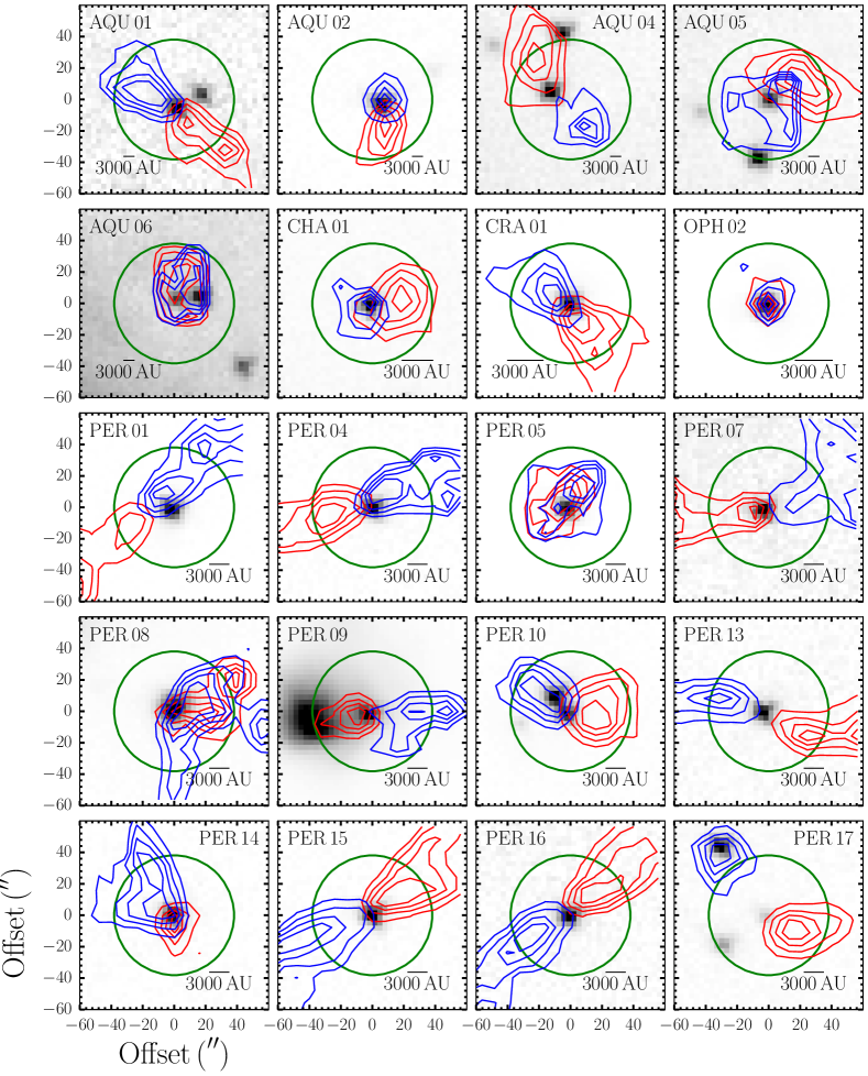
Figure 17: Outflow maps. The grey-scale images show the 70 $\mu$m continuum emission from Herschel, while the red and blue contours show the outflow lobes detected in ¹²CO $J$=3$-$2. The levels for the contours are at 20, 40, 60 and 80$\%$ of the maximum velocity-integrated emission. The green circle indicates the HIFI beam for the H₂O 1${}_{10}-$1₀₁ transition. All maps show a region of 2^′ $\times$2^′ centred on the source position. The black scale-bar in the lower panel of each figure indicates 3000 AU at the distance of the source.

Figure A.17 (Cont.): Outflow maps. The grey-scale images show the 70 $\mu$m continuum emission from Herschel, while the red and blue contours show the outflow lobes detected in ¹²CO $J$=3$-$2. The levels for the contours are at 20, 40, 60 and 80$\%$ of the maximum velocity-integrated emission. The green circle indicates the HIFI beam for the H₂O 1${}_{10}-$1₀₁ transition. All maps show a region of 2^′ $\times$2^′ centred on the source position. The black scale-bar in the lower panel of each figure indicates 3000 AU at the distance of the source.

Table A.9: Outflow properties.

Name	$i$	Lobe	$\varv_{in}$	$\varv_{out}$	$\mid\varv_{max}\mid$	$M_{\mathrm{out}}$	$P_{\mathrm{out}}$	$E_{\mathrm{out}}$	$R_{\mathrm{CO}}$	$t_{\mathrm{dyn}}$	$F_{\mathrm{CO}}$	$\dot{M}_{\mathrm{out}}$
	(∘)		(km s-1)	(km s-1)	(km s-1)	($M_{\odot}$)	($M_{\odot}$ km s-1)	(ergs)	(103 AU)	(103 yrs)	($M_{\odot}$ yr-1 km s-1)	($M_{\odot}$ yr-1)
AQU 01	70	R	11.0	33.5	26.1	1.6$\times$10-02	1.5$\times$10-01	1.8$\times$10+43	15.0	02.7	3.9$\times$10-04	4.2$\times$10-05
		B	03.0	$-$30.0$-$	37.4	2.2$\times$10-02	2.2$\times$10-01	3.3$\times$10+43	28.1	03.6	4.5$\times$10-04	4.3$\times$10-05
AQU 02	30	R	10.5	25.0	17.5	7.4$\times$10-03	4.2$\times$10-02	3.1$\times$10+42	16.4	04.4	2.7$\times$10-05	4.6$\times$10-06
		B	04.5	0$-$8.5$-$	16.0	4.8$\times$10-03	3.1$\times$10-02	2.6$\times$10+42	05.5	01.6	5.4$\times$10-05	8.2$\times$10-06
AQU 03	$-$	$-$	$-$	$-$	$-$	$-$	$-$	$-$	$-$	$-$	$-$	$-$
AQU 04	70	R	11.0	17.5	9.9	7.7$\times$10-03	3.7$\times$10-02	1.9$\times$10+42	29.2	14.0	1.9$\times$10-05	3.9$\times$10-06
		B	02.5	0$-$1.0$-$	08.6	8.7$\times$10-04	5.4$\times$10-03	3.4$\times$10+41	10.0	05.5	6.9$\times$10-06	1.1$\times$10-06
AQU 05	30	R	11.0	18.5	11.2	1.9$\times$10-02	9.8$\times$10-02	5.5$\times$10+42	15.1	06.4	4.3$\times$10-05	8.2$\times$10-06
		B	02.5	0$-$4.0$-$	11.3	1.5$\times$10-03	1.2$\times$10-02	9.8$\times$10+41	16.4	06.8	4.8$\times$10-06	6.1$\times$10-07
AQU 06	10	R	11.0	18.5	10.2	2.7$\times$10-03	1.2$\times$10-02	6.5$\times$10+41	05.3	02.5	6.0$\times$10-06	1.3$\times$10-06
		B	03.0	0$-$3.5$-$	11.8	1.1$\times$10-03	9.1$\times$10-03	7.7$\times$10+41	05.3	02.2	5.0$\times$10-06	6.3$\times$10-07
CHA 01	30	R	07.5	12.0	07.1	9.7$\times$10-04	3.7$\times$10-03	1.5$\times$10+41	10.7	07.1	1.4$\times$10-06	3.8$\times$10-07
		B	03.0	02.0	02.9	8.8$\times$10-05	2.0$\times$10-04	4.8$\times$10+39	04.8	07.8	7.3$\times$10-08	3.2$\times$10-08
CHA 02	$-$	$-$	$-$	$-$	$-$	$-$	$-$	$-$	$-$	$-$	$-$	$-$
CRA 01	50	R	07.3	22.8	17.1	1.5$\times$10-03	6.8$\times$10-03	4.8$\times$10+41	18.7	05.2	5.7$\times$10-06	1.3$\times$10-06
		B	03.8	$-$16.7$-$	22.4	1.4$\times$10-03	6.2$\times$10-03	4.2$\times$10+41	27.9	05.9	4.6$\times$10-06	1.0$\times$10-06
OPH 01	$-$	$-$	$-$	$-$	$-$	$-$	$-$	$-$	$-$	$-$	$-$	$-$
OPH 02	10	R	07.0	10.5	06.3	5.1$\times$10-05	1.9$\times$10-04	7.3$\times$10+39	09.2	07.0	3.2$\times$10-08	8.7$\times$10-09
		B	01.0	0$-$4.0$-$	08.2	9.3$\times$10-05	3.7$\times$10-04	1.6$\times$10+40	11.8	06.8	6.6$\times$10-08	1.6$\times$10-08
PER 01	70	R	07.2	49.2	45.2	2.4$\times$10-02	2.1$\times$10-01	3.2$\times$10+43	41.9	04.4	3.4$\times$10-04	3.9$\times$10-05
		B	0$-$2.3$-$	$-$36.3$-$	40.3	1.0$\times$10-02	1.5$\times$10-01	2.9$\times$10+43	15.2	01.8	5.9$\times$10-04	4.2$\times$10-05
PER 02	$-$	$-$	$-$	$-$	$-$	$-$	$-$	$-$	$-$	$-$	$-$	$-$
PER 04	50	R	06.2	12.7	07.5	2.3$\times$10-03	5.9$\times$10-03	2.0$\times$10+41	27.9	17.6	1.5$\times$10-06	5.8$\times$10-07
		B	01.7	0$-$1.8$-$	07.0	2.8$\times$10-04	1.3$\times$10-03	6.2$\times$10+40	14.2	9.6	5.9$\times$10-07	1.3$\times$10-07
PER 05	10	R	12.7	17.7	10.5	2.5$\times$10-04	1.8$\times$10-03	1.4$\times$10+41	13.9	06.3	3.5$\times$10-07	4.8$\times$10-08
		B	03.2	0$-$1.3$-$	08.5	3.4$\times$10-04	1.8$\times$10-03	1.0$\times$10+41	13.9	07.7	2.9$\times$10-07	5.4$\times$10-08
PER 06	$-$	$-$	$-$	$-$	$-$	$-$	$-$	$-$	$-$	$-$	$-$	$-$
PER 07	70	R	11.2	20.7	13.4	1.7$\times$10-03	1.1$\times$10-02	7.3$\times$10+41	29.2	10.4	7.2$\times$10-06	1.2$\times$10-06
		B	02.2	0$-$5.3$-$	12.6	2.4$\times$10-03	1.6$\times$10-02	1.2$\times$10+42	17.4	06.6	1.8$\times$10-05	2.6$\times$10-06
PER 08	10	R	15.5	21.5	13.8	5.4$\times$10-04	5.1$\times$10-03	5.0$\times$10+41	12.7	04.4	1.4$\times$10-06	1.5$\times$10-07
		B	0$-$0.5$-$	$-$14.5$-$	22.2	3.4$\times$10-03	3.6$\times$10-02	4.1$\times$10+42	15.1	03.2	1.3$\times$10-05	1.2$\times$10-06
PER 09	70	R	13.0	25.0	17.5	5.3$\times$10-04	4.9$\times$10-03	5.1$\times$10+41	14.6	04.0	8.8$\times$10-06	9.6$\times$10-07
		B	00.5	$-$16.0$-$	23.5	7.6$\times$10-04	9.3$\times$10-03	1.3$\times$10+42	14.1	02.8	2.3$\times$10-05	1.9$\times$10-06
PER 10	50	R	13.2	32.2	23.6	1.3$\times$10-02	9.6$\times$10-02	8.7$\times$10+42	14.2	02.9	1.5$\times$10-04	1.9$\times$10-05
		B	02.2	$-$14.8$-$	23.4	6.1$\times$10-03	6.1$\times$10-02	6.8$\times$10+42	24.9	05.0	5.3$\times$10-05	5.4$\times$10-06
PER 12	$-$	$-$	$-$	$-$	$-$	$-$	$-$	$-$	$-$	$-$	$-$	$-$
PER 13	70	R	10.7	22.2	14.3	4.1$\times$10-03	1.9$\times$10-02	1.1$\times$10+42	14.2	04.7	2.9$\times$10-05	6.1$\times$10-06
		B	05.7	0$-$4.3$-$	12.2	1.8$\times$10-03	7.9$\times$10-03	4.8$\times$10+41	27.0	10.4	5.4$\times$10-06	1.2$\times$10-06
PER 14	50	R	09.0	20.0	13.8	3.0$\times$10-04	1.7$\times$10-03	1.1$\times$10+41	04.0	01.4	5.3$\times$10-06	9.7$\times$10-07
		B	04.5	0$-$9.0$-$	15.2	5.3$\times$10-03	2.0$\times$10-02	1.0$\times$10+42	27.9	08.7	9.9$\times$10-06	2.7$\times$10-06
PER 15	70	R	9.7	28.2	21.2	1.0$\times$10-02	6.4$\times$10-02	5.4$\times$10+42	17.4	03.9	1.2$\times$10-04	1.8$\times$10-05
		B	01.2	$-$25.3$-$	32.3	4.9$\times$10-03	5.3$\times$10-02	7.2$\times$10+42	37.0	05.4	6.9$\times$10-05	6.4$\times$10-06
PER 16	70	R	09.2	23.2	16.2	4.6$\times$10-03	2.3$\times$10-02	1.7$\times$10+42	17.4	05.1	3.3$\times$10-05	6.4$\times$10-06
		B	02.7	0$-$6.3$-$	13.3	2.2$\times$10-03	1.4$\times$10-02	1.1$\times$10+42	37.0	13.2	7.8$\times$10-06	1.2$\times$10-06
PER 17	50	R	10.8	30.3	23.7	5.2$\times$10-03	3.8$\times$10-02	3.4$\times$10+42	12.8	02.6	6.6$\times$10-05	8.9$\times$10-06
		B	02.8	$-$20.2$-$	26.8	7.2$\times$10-03	5.2$\times$10-02	4.9$\times$10+42	30.1	05.3	4.3$\times$10-05	5.9$\times$10-06
PER 18	70	R	10.8	32.3	25.6	2.1$\times$10-03	2.1$\times$10-02	2.7$\times$10+42	32.4	06.0	2.5$\times$10-05	2.4$\times$10-06
		B	02.8	0$-$5.7$-$	12.4	7.0$\times$10-04	3.9$\times$10-03	2.5$\times$10+41	12.7	04.9	5.7$\times$10-06	1.0$\times$10-06
PER 19	50	R	9.7	15.7	09.0	2.4$\times$10-03	9.3$\times$10-03	3.9$\times$10+41	17.4	09.2	4.5$\times$10-06	1.2$\times$10-06
		B	02.7	0$-$4.3$-$	11.0	6.0$\times$10-04	3.2$\times$10-03	1.9$\times$10+41	11.8	05.1	2.8$\times$10-06	5.2$\times$10-07
PER 20	50	R	11.2	50.2	41.3	5.6$\times$10-03	6.0$\times$10-02	1.2$\times$10+43	11.8	01.4	1.9$\times$10-04	1.8$\times$10-05
		B	06.2	$-$13.8$-$	22.7	4.7$\times$10-03	3.8$\times$10-02	4.2$\times$10+42	28.1	05.9	2.8$\times$10-05	3.5$\times$10-06

Table A.9 (Cont.): Outflow properties.

Name	$i$	Lobe	$\varv_{in}$	$\varv_{out}$	$\mid\varv_{max}\mid$	$M_{\mathrm{out}}$	$P_{\mathrm{out}}$	$E_{\mathrm{out}}$	$R_{\mathrm{CO}}$	$t_{\mathrm{dyn}}$	$F_{\mathrm{CO}}$	$\dot{M}_{\mathrm{out}}$
	(∘)		(km s-1)	(km s-1)	(km s-1)	($M_{\odot}$)	($M_{\odot}$ km s-1)	(ergs)	(103 AU)	(103 yrs)	($M_{\odot}$ yr-1 km s-1)	($M_{\odot}$ yr-1)
PER 21	50	R	11.2	28.2	19.5	4.0$\times$10-03	2.5$\times$10-02	2.3$\times$10+42	26.4	06.4	1.7$\times$10-05	2.7$\times$10-06
		B	04.7	$-$15.8$-$	24.5	2.4$\times$10-03	2.2$\times$10-02	2.6$\times$10+42	10.8	02.1	4.6$\times$10-05	5.1$\times$10-06
PER 22	30	R	11.2	18.2	08.5	5.4$\times$10-03	1.2$\times$10-02	3.2$\times$10+41	21.9	12.3	2.7$\times$10-06	1.2$\times$10-06
		B	06.2	03.2	06.5	9.0$\times$10-04	3.6$\times$10-03	1.5$\times$10+41	10.8	07.8	1.3$\times$10-06	3.2$\times$10-07
SCO 01	$-$	$-$	$-$	$-$	$-$	$-$	$-$	$-$	$-$	$-$	$-$	$-$
SERS 01	50	R	11.0	18.5	10.3	1.5$\times$10-02	6.4$\times$10-02	3.1$\times$10+42	19.9	09.1	3.1$\times$10-05	7.2$\times$10-06
		B	03.5	$-$15.0$-$	23.2	1.6$\times$10-02	1.2$\times$10-01	1.0$\times$10+43	32.4	06.6	7.8$\times$10-05	1.1$\times$10-05
SERS 02	50	R	13.5	40.5	32.7	1.0$\times$10-01	9.9$\times$10-01	1.2$\times$10+44	07.9	01.1	3.8$\times$10-03	3.9$\times$10-04
		B	01.0	$-$18.5$-$	26.3	3.0$\times$10-02	3.2$\times$10-01	3.9$\times$10+43	26.4	04.8	2.9$\times$10-04	2.8$\times$10-05
TAU 01	50	R	08.3	16.8	10.0	2.1$\times$10-03	5.4$\times$10-03	1.8$\times$10+41	26.4	12.6	1.9$\times$10-06	7.5$\times$10-07
		B	04.8	0$-$6.7$-$	13.5	2.6$\times$10-04	8.5$\times$10-04	3.9$\times$10+40	03.4	01.2	3.2$\times$10-06	9.5$\times$10-07
TAU 02	50	R	08.0	11.5	04.9	3.1$\times$10-04	5.6$\times$10-04	1.2$\times$10+40	18.5	17.9	1.4$\times$10-07	7.7$\times$10-08
		B	05.0	0$-$0.0$-$	06.6	2.5$\times$10-04	6.2$\times$10-04	1.9$\times$10+40	11.8	08.5	3.2$\times$10-07	1.3$\times$10-07
TAU 03	50	R	08.5	14.0	06.6	6.3$\times$10-04	1.3$\times$10-03	3.4$\times$10+40	11.8	08.5	6.5$\times$10-07	3.2$\times$10-07
		B	04.5	03.0	04.4	3.5$\times$10-05	1.1$\times$10-04	3.5$\times$10+39	28.1	30.2	1.6$\times$10-08	5.0$\times$10-09
TAU 04	50	R	07.5	18.0	11.7	9.5$\times$10-04	2.9$\times$10-03	1.3$\times$10+41	16.2	06.6	1.9$\times$10-06	6.3$\times$10-07
		B	05.5	01.0	05.3	4.7$\times$10-04	6.5$\times$10-04	1.2$\times$10+40	27.9	24.8	1.2$\times$10-07	8.3$\times$10-08
TAU 06	30	R	09.0	14.0	06.8	5.4$\times$10-04	1.5$\times$10-03	4.6$\times$10+40	26.4	18.4	2.2$\times$10-07	8.3$\times$10-08
		B	05.5	00.0	07.2	5.3$\times$10-04	1.3$\times$10-03	3.7$\times$10+40	23.6	15.5	2.3$\times$10-07	9.5$\times$10-08
TAU 07	$-$	$-$	$-$	$-$	$-$	$-$	$-$	$-$	$-$	$-$	$-$	$-$
TAU 08	$-$	$-$	$-$	$-$	$-$	$-$	$-$	$-$	$-$	$-$	$-$	$-$
TAU 09	$-$	$-$	$-$	$-$	$-$	$-$	$-$	$-$	$-$	$-$	$-$	$-$
W40 01	$-$	$-$	$-$	$-$	$-$	$-$	$-$	$-$	$-$	$-$	$-$	$-$
W40 02	70	R	11.5	19.0	14.2	2.4$\times$10-03	2.1$\times$10-02	1.9$\times$10+42	15.8	05.3	2.8$\times$10-05	3.2$\times$10-06
		B	02.5	0$-$6.5$-$	11.3	1.1$\times$10-02	4.8$\times$10-02	2.5$\times$10+42	26.4	11.0	3.1$\times$10-05	6.9$\times$10-06
W40 03	$-$	$-$	$-$	$-$	$-$	$-$	$-$	$-$	$-$	$-$	$-$	$-$
W40 04	$-$	$-$	$-$	$-$	$-$	$-$	$-$	$-$	$-$	$-$	$-$	$-$
W40 05	$-$	$-$	$-$	$-$	$-$	$-$	$-$	$-$	$-$	$-$	$-$	$-$
W40 06	$-$	$-$	$-$	$-$	$-$	$-$	$-$	$-$	$-$	$-$	$-$	$-$
W40 07	50	R	10.5	26.0	18.6	5.4$\times$10-03	4.6$\times$10-02	5.1$\times$10+42	26.4	06.7	3.0$\times$10-05	3.5$\times$10-06
		B	03.0	0$-$4.0$-$	11.4	1.2$\times$10-03	8.7$\times$10-03	6.9$\times$10+41	04.2	01.7	2.2$\times$10-05	3.0$\times$10-06

A.5 Mass accretion and loss

Table 18 presents the calculated mass accretion rates for all WILL, WISH and DIGIT sources, calculated as discussed in Sect. 4.4 using Eqn. 6, as well as the observed luminosity in the [O i] 63 $\mu$m transition and the mass-loss rate in the wind derived using the relation from Hollenbach (1985), given in Eqn. 7. $L\mathrm{[OI\,63\mu m]}$ is not given for OPH 01, W40 01 and W40 03$-$06 as the detections in [O i] towards these sources are almost certainly due to PDR emission.

Table A.10: Mass-accretion rate, the luminosity of [O i] in the 63 $\mu$m line, and mass-loss rate calculated from it.

Name	$\dot{M}_{\mathrm{acc}}$	$L$[O i 63$\mu$m]	$\dot{M}_{\mathrm{w}}$		Name	$\dot{M}_{\mathrm{acc}}$	$L$[O i 63$\mu$m]	$\dot{M}_{\mathrm{w}}$
	($M_{\odot}$ yr-1)	($L_{\odot}$)	($M_{\odot}$ yr-1)			($M_{\odot}$ yr-1)	($L_{\odot}$)	($M_{\odot}$ yr-1)
AQU 01	1.7$\times$10-06	8.3$\times$10-04	8.3$\times$10-08		AQU 02	5.9$\times$10-06	8.2$\times$10-04	8.2$\times$10-08
AQU 03	$-$	$-$	$-$		AQU 04	8.4$\times$10-07	$-$	$-$
AQU 05	1.6$\times$10-06	$-$	$-$		AQU 06	8.1$\times$10-07	$-$	$-$
CHA 01	$-$	3.7$\times$10-04	3.7$\times$10-08		CHA 02	2.3$\times$10-07	8.7$\times$10-05	8.7$\times$10-09
CRA 01	1.6$\times$10-06	1.2$\times$10-03	1.2$\times$10-07		OPH 01	$-$	2.9$\times$10-03	$-$
OPH 02	1.1$\times$10-06	5.2$\times$10-04	5.2$\times$10-08		PER 01	2.9$\times$10-06	3.4$\times$10-03	3.4$\times$10-07
PER 02	6.0$\times$10-06	7.8$\times$10-03	7.8$\times$10-07		PER 04	7.6$\times$10-07	5.3$\times$10-04	5.3$\times$10-08
PER 05	1.4$\times$10-06	2.8$\times$10-04	2.8$\times$10-08		PER 06	9.2$\times$10-07	1.6$\times$10-03	1.6$\times$10-07
PER 07	4.6$\times$10-07	1.2$\times$10-03	1.2$\times$10-07		PER 08	2.2$\times$10-06	1.1$\times$10-02	1.1$\times$10-06
PER 09	2.9$\times$10-06	$-$	$-$		PER 10	3.9$\times$10-06	$-$	$-$
PER 12	6.9$\times$10-07	1.1$\times$10-04	1.1$\times$10-08		PER 13	4.4$\times$10-07	$-$	$-$
PER 14	2.4$\times$10-07	4.6$\times$10-04	4.6$\times$10-08		PER 15	1.1$\times$10-06	2.1$\times$10-04	2.1$\times$10-08
PER 16	7.4$\times$10-07	2.6$\times$10-04	2.6$\times$10-08		PER 17	2.3$\times$10-08	1.4$\times$10-04	1.4$\times$10-08
PER 18	3.4$\times$10-07	1.8$\times$10-03	1.8$\times$10-07		PER 19	1.4$\times$10-07	1.8$\times$10-03	1.8$\times$10-07
PER 20	1.4$\times$10-06	1.9$\times$10-03	1.9$\times$10-07		PER 21	1.2$\times$10-06	8.6$\times$10-04	8.6$\times$10-08
PER 22	1.6$\times$10-06	1.0$\times$10-03	1.0$\times$10-07		SCO 01	$-$	2.8$\times$10-04	2.8$\times$10-08
SERS 01	1.1$\times$10-05	2.8$\times$10-03	2.8$\times$10-07		SERS 02	4.7$\times$10-05	$-$	$-$
TAU 01	2.0$\times$10-07	7.6$\times$10-04	7.6$\times$10-08		TAU 02	6.1$\times$10-08	1.1$\times$10-04	1.1$\times$10-08
TAU 03	$-$	5.4$\times$10-05	5.4$\times$10-09		TAU 04	1.8$\times$10-07	4.5$\times$10-04	4.5$\times$10-08
TAU 06	7.3$\times$10-08	9.6$\times$10-05	9.6$\times$10-09		TAU 07	$-$	3.5$\times$10-04	3.5$\times$10-08
TAU 08	$-$	$-$	$-$		TAU 09	$-$	2.9$\times$10-04	2.9$\times$10-08
W40 01	$-$	3.1$\times$10-04	$-$		W40 02	2.1$\times$10-05	5.4$\times$10-02	5.4$\times$10-06
W40 03	$-$	1.5$\times$10-01	$-$		W40 04	$-$	1.1$\times$10-01	$-$
W40 05	$-$	7.8$\times$10-02	$-$		W40 06	$-$	0.0$\times$10+00	$-$
W40 07	2.3$\times$10-06	5.4$\times$10-04	5.4$\times$10-08		L1448-MM	5.8$\times$10-06	2.2$\times$10-03	2.2$\times$10-07
IRAS03245+3002	4.2$\times$10-06	6.4$\times$10-04	6.4$\times$10-08		L1455-IRS3	4.7$\times$10-08	5.0$\times$10-04	5.0$\times$10-08
NGC1333-IRAS2A	2.3$\times$10-05	$-$	$-$		NGC1333-IRAS3A	5.4$\times$10-06	$-$	$-$
NGC1333-IRAS4A	5.9$\times$10-06	1.5$\times$10-03	$-$		NGC1333-IRAS4B	2.9$\times$10-06	1.3$\times$10-04	1.3$\times$10-08
IRAS03301+3111	5.3$\times$10-07	3.6$\times$10-04	3.6$\times$10-08		B1 a	3.5$\times$10-07	1.9$\times$10-04	1.9$\times$10-08
B1 c	3.3$\times$10-06	$-$	$-$		L1489	4.9$\times$10-07	2.2$\times$10-04	2.2$\times$10-08
L1551-IRS5	2.9$\times$10-06	9.7$\times$10-03	9.7$\times$10-07		TMR1	4.9$\times$10-07	1.1$\times$10-03	1.1$\times$10-07
TMC1A	3.5$\times$10-07	3.3$\times$10-03	3.3$\times$10-07		L1527	1.2$\times$10-06	1.8$\times$10-03	1.8$\times$10-07
TMC1	1.2$\times$10-07	1.5$\times$10-03	1.5$\times$10-07		IRAM04191	7.1$\times$10-08	2.4$\times$10-04	2.4$\times$10-08
HH46	3.6$\times$10-06	5.1$\times$10-03	5.1$\times$10-07		Ced110-IRS4	5.2$\times$10-07	1.3$\times$10-03	1.3$\times$10-07
BHR71	9.6$\times$10-06	3.4$\times$10-03	3.4$\times$10-07		IRAS12496	4.6$\times$10-06	5.9$\times$10-03	5.9$\times$10-07
IRAS15398	1.0$\times$10-06	3.0$\times$10-03	3.0$\times$10-07		GSS30	1.8$\times$10-06	5.1$\times$10-03	5.1$\times$10-07
VLA1623-243	1.7$\times$10-06	1.3$\times$10-03	1.3$\times$10-07		WL12	2.1$\times$10-07	7.9$\times$10-04	7.9$\times$10-08
Elias29	1.8$\times$10-06	4.0$\times$10-03	4.0$\times$10-07		IRS44	6.6$\times$10-07	4.8$\times$10-04	4.8$\times$10-08
IRS46	6.5$\times$10-08	1.5$\times$10-04	1.5$\times$10-08		IRS63	1.3$\times$10-07	3.3$\times$10-04	3.3$\times$10-08
RNO91	3.4$\times$10-07	1.3$\times$10-03	1.3$\times$10-07		L483	6.6$\times$10-06	1.1$\times$10-03	1.1$\times$10-07
Ser-SMM1	7.1$\times$10-05	4.0$\times$10-03	4.0$\times$10-07		Ser-SMM4	4.4$\times$10-06	1.8$\times$10-02	1.8$\times$10-06
Ser-SMM3	1.2$\times$10-05	1.1$\times$10-02	1.1$\times$10-06		RCrA-IRS5A	9.2$\times$10-07	1.2$\times$10-03	1.2$\times$10-07
RCrA I7A	1.2$\times$10-05	8.9$\times$10-03	8.9$\times$10-07		RCrA I7B	6.0$\times$10-06	2.4$\times$10-03	2.4$\times$10-07
HH100	2.3$\times$10-06	$-$	$-$		L723	2.3$\times$10-06	1.3$\times$10-04	1.3$\times$10-08
B335	2.1$\times$10-06	2.5$\times$10-04	2.5$\times$10-08		L1157	3.0$\times$10-06	3.3$\times$10-04	3.3$\times$10-08

A.6 Ground-based line fitting

Table A.11: Species and transitions targeted during the ground-based spectral follow-up.

Species	Transition	Rest Frequency	Eu/$k_{\mathrm{b}}$	$A_{\mathrm{ul}}$	$n_{\mathrm{cr}}$	JCMT $\eta_{mb}$	APEX $\eta_{mb}$	JCMT $\theta_{mb}$	APEX $\theta_{mb}$	Median $\sigma_{\mathrm{rms}}$
		(GHz)	(K)	(s-1)	(cm-3)			(′′)	(′′)	(K)
CO	2$-$1	230.53800	16.60	6.91$\times$10-7	6$\times$103	$-$	0.75	$-$	27.3	0.41
13CO	2$-$1	220.39868	15.87	6.04$\times$10-7	5$\times$103	$-$	0.75	$-$	28.5	0.08
C18O	2$-$1	219.56035	15.81	6.01$\times$10-7	5$\times$103	$-$	0.75	$-$	28.6	0.08
C17O	2$-$1	224.71439	16.18	6.43$\times$10-7	6$\times$103	$-$	0.75	$-$	28.0	0.08
CO	3$-$2	345.79599	33.19	2.50$\times$10-6	2$\times$104	0.63	0.73	14.5	18.2	0.09
13CO	3$-$2	330.58797	31.73	2.18$\times$10-6	1$\times$104	0.63	0.73	15.2	19.0	0.22
C18O	3$-$2	329.33055	31.61	2.17$\times$10-6	1$\times$104	0.63	0.73	15.3	19.1	0.30
C17O	3$-$2	337.06113	32.35	2.32$\times$10-6	1$\times$104	$-$	0.73	$-$	18.7	0.09
CO	4$-$3	461.04077	55.32	6.13$\times$10-6	3$\times$104	$-$	0.60	$-$	13.6	0.12
HCO+	4$-$3	356.73429	42.80	3.63$\times$10-3	2$\times$107	0.63	0.73	14.1	17.6	0.28
H13CO+	4$-$3	346.99834	41.63	3.29$\times$10-3	2$\times$107	0.63	0.73	14.5	18.2	0.13

Table 19 presents the basic properties of all transitions observed with the JCMT and APEX. Gaussian fitting was performed for the central spectra of all sources for ¹³CO, C¹⁸O, HCO⁺ and H¹³CO⁺ in order to determine line-widths and central velocities. The $\varv_{\mathrm{LSR}}$ for each source is defined as the peak position of the fit to the C¹⁸O $J$=3$-$2 central spectrum. For the four sources where this is not detected, three (SCO 01, TAU 03, TAU 07) were also observed and detected in ¹³CO $J$=3$-$2, so the fit to this line is used instead. For the remaining source (TAU 08) we use the velocity derived by Caselli et al. (2002) from N₂H⁺ $J$=1$-$0 observations. The integrated intensity of the lines is measured over a window of $\pm$3 FWHM.

For the optically thick HCO⁺ and ¹³CO, we also quantify any blue/red asymmetry by calculating $\delta\varv$ as defined by Mardones et al. (1997) using Eqn. 11. For most sources, we use the peak of the Gaussian fit to the line, but in the case of five sources (AQU 02, PER 04, SERS 01, SERS 02 and TAU 09), the position of the maximum intensity is used in this calculation for HCO⁺ because strong self-absorption or a broad, fainter second component skews the Gaussian fit away from the maximum intensity.

The results for all sources are presented in Table 20, and Fig. A.18 shows the central HCO⁺ and C¹⁸O spectra for all sources.

Figure A.18: Overview of the central HCO⁺ $J$=4$-$3 and C¹⁸O $J$=3$-$2 spectra shown in black and red respectively. All have been recentred so that the source velocity is at zero. Sources that are considered blue-skewed (i.e. $\delta\varv<-$0.25) have their names in blue, while those considered red-skewed (i.e. $\delta\varv>$0.25) have their names in red. The number in the upper-right corner of each panel indicates what factor the spectra have been multiplied by.

Figure A.18 (Cont.): Overview of the central HCO⁺ $J$=4$-$3 and C¹⁸O $J$=3$-$2 spectra shown in black and red respectively. All have been recentred so that the source velocity is at zero. Sources that are considered blue-skewed (i.e. $\delta\varv<-$0.25) have their names in blue, while those considered red-skewed (i.e. $\delta\varv>$0.25) have their names in red. The number in the upper-right corner of each panel indicates what factor the spectra have been multiplied by.

Table A.12: Ground-based spectral results.

Name	Molecule	Transition	$\sigma_{\mathrm{rms}}$	$\varv_{\mathrm{max}}$	Tmax	$\varv_{\mathrm{peak}}$	Tpeak	FWHM	$\int T_{\mathrm{MB}}\,\mathrm{d}\varv$	$\delta\varv$
			(K)	(km s-1)	(K)	(km s-1)	(K)	(km s-1)	(K km s-1)	(km s-1)
AQU 01	13CO	3$-$2	0.25	7.2	02.33	7.3$\pm$0.1	02.1$\pm$0.2	1.9$\pm$0.2	04.23$\pm$0.57	$-$0.07$\pm$0.03$-$
	C18O	3$-$2	0.32	7.4	01.48	7.4$\pm$0.2	01.2$\pm$0.4	1.1$\pm$0.4	01.34$\pm$0.74	0.00$\pm$0.01
	HCO+	4$-$3	0.39	7.0	02.08	7.4$\pm$0.2	01.6$\pm$0.2	2.6$\pm$0.4	04.56$\pm$0.89	$-$0.04$\pm$0.01$-$
	H13CO+	4$-$3	0.18	$-$	$<$0.55	$-$	$-$	$-$	$-$	$-$
AQU 02	13CO	3$-$2	0.21	7.6	04.47	7.5$\pm$0.1	04.2$\pm$0.2	1.8$\pm$0.1	07.95$\pm$0.48	$-$0.01$\pm$0.01$-$
	C18O	3$-$2	0.26	7.8	01.19	7.5$\pm$0.2	01.0$\pm$0.3	1.2$\pm$0.4	01.38$\pm$0.60	0.00$\pm$0.01
	HCO+	4$-$3	0.30	7.4	04.63	7.6$\pm$0.1	04.7$\pm$0.3	2.7$\pm$0.1	13.28$\pm$0.94	$-$0.09$\pm$0.03 $-$
AQU 03	13CO	3$-$2	0.21	7.4	02.33	7.1$\pm$0.1	02.2$\pm$0.2	1.4$\pm$0.2	03.27$\pm$0.49	0.02$\pm$0.01
	C18O	3$-$2	0.28	7.4	01.20	7.1$\pm$0.2	01.1$\pm$0.4	1.1$\pm$0.4	01.22$\pm$0.65	0.00$\pm$0.01
	HCO+	4$-$3	0.28	$-$	$<$0.85	$-$	$-$	$-$	$-$	$-$
	H13CO+	4$-$3	0.25	$-$	$<$0.75	$-$	$-$	$-$	$-$	$-$
AQU 04	13CO	3$-$2	0.22	7.4	03.90	7.5$\pm$0.1	03.2$\pm$0.1	2.8$\pm$0.1	09.29$\pm$0.55	$-$0.01$\pm$0.01$-$
	C18O	3$-$2	0.36	7.6	02.03	7.6$\pm$0.1	01.8$\pm$0.3	1.6$\pm$0.3	03.07$\pm$0.83	0.00$\pm$0.01
	HCO+	4$-$3	0.33	8.2	02.52	8.1$\pm$0.1	02.1$\pm$0.4	1.3$\pm$0.3	02.81$\pm$0.78	0.33$\pm$0.07
	H13CO+	4$-$3	0.19	$-$	$<$0.56	$-$	$-$	$-$	$-$	$-$
AQU 05	13CO	3$-$2	0.27	7.0	02.79	7.4$\pm$0.1	01.9$\pm$0.1	2.9$\pm$0.2	05.91$\pm$0.66	0.10$\pm$0.03
	C18O	3$-$2	0.30	7.4	01.36	7.3$\pm$0.2	01.4$\pm$0.4	1.2$\pm$0.4	01.72$\pm$0.69	0.00$\pm$0.01
	HCO+	4$-$3	0.31	8.2	01.44	8.2$\pm$0.2	01.4$\pm$0.3	1.3$\pm$0.4	01.98$\pm$0.71	0.70$\pm$0.21
	H13CO+	4$-$3	0.14	$-$	$<$0.43	$-$	$-$	$-$	$-$	$-$
AQU 06	13CO	3$-$2	0.25	8.4	02.52	8.3$\pm$0.1	02.0$\pm$0.2	1.9$\pm$0.2	04.11$\pm$0.57	0.11$\pm$0.07
	C18O	3$-$2	0.33	8.4	01.19	8.3$\pm$0.2	01.3$\pm$0.7	0.6$\pm$0.4	00.90$\pm$0.76	0.00$\pm$0.01
	HCO+	4$-$3	0.29	8.4	02.02	8.4$\pm$0.1	01.8$\pm$0.4	1.0$\pm$0.3	01.96$\pm$0.67	0.22$\pm$0.14
	H13CO+	4$-$3	0.16	$-$	$<$0.47	$-$	$-$	$-$	$-$	$-$
CHA 01	13CO	2$-$1	0.08	5.2	06.63	4.9$\pm$0.1	05.9$\pm$0.2	1.5$\pm$0.1	09.62$\pm$0.43	$-$0.01$\pm$0.01$-$
	C18O	2$-$1	0.08	4.7	04.44	4.7$\pm$0.1	04.8$\pm$0.3	0.7$\pm$0.1	03.63$\pm$0.39	0.00$\pm$0.01
	C17O	2$-$1	0.08	5.2	01.47	5.2$\pm$0.1	01.4$\pm$0.3	0.7$\pm$0.2	01.09$\pm$0.37	0.00$\pm$0.01
	13CO	3$-$2	0.12	5.1	04.04	4.8$\pm$0.1	03.7$\pm$0.2	1.6$\pm$0.1	06.43$\pm$0.55	$-$0.13$\pm$0.05$-$
	C18O	3$-$2	0.16	4.8	01.94	4.9$\pm$0.1	02.2$\pm$0.7	0.6$\pm$0.2	01.49$\pm$0.77	0.00$\pm$0.01
	C17O	3$-$2	0.08	5.1	00.45	4.8$\pm$0.2	00.4$\pm$0.2	0.9$\pm$0.6	00.43$\pm$0.35	0.00$\pm$0.01
	HCO+	4$-$3	0.07	$-$	$<$0.20	$-$	$-$	$-$	$-$	$-$
	H13CO+	4$-$3	0.06	$-$	$<$0.18	$-$	$-$	$-$	$-$	$-$
CHA 02	13CO	2$-$1	0.09	3.5	04.66	3.2$\pm$0.1	04.7$\pm$0.2	1.3$\pm$0.1	06.71$\pm$0.47	0.18$\pm$0.07
	C18O	2$-$1	0.08	3.1	03.60	3.0$\pm$0.1	03.7$\pm$0.3	0.8$\pm$0.1	02.98$\pm$0.43	0.00$\pm$0.01
	C17O	2$-$1	0.08	3.5	01.36	3.5$\pm$0.1	01.2$\pm$0.3	0.8$\pm$0.2	01.06$\pm$0.37	0.00$\pm$0.01
	13CO	3$-$2	0.13	3.6	02.24	3.0$\pm$0.1	02.0$\pm$0.2	1.8$\pm$0.2	03.84$\pm$0.59	$-$0.01$\pm$0.01$-$
	C18O	3$-$2	0.17	3.0	01.54	3.0$\pm$0.1	01.6$\pm$0.5	0.9$\pm$0.3	01.47$\pm$0.75	0.00$\pm$0.01
	C17O	3$-$2	0.10	3.3	00.40	3.2$\pm$0.3	00.4$\pm$0.3	0.8$\pm$0.8	00.31$\pm$0.43	0.00$\pm$0.01
	HCO+	4$-$3	0.11	3.0	00.76	3.0$\pm$0.2	00.6$\pm$0.3	1.0$\pm$0.6	00.65$\pm$0.49	$-$0.04$\pm$0.02$-$
	H13CO+	4$-$3	0.10	$-$	$<$0.29	$-$	$-$	$-$	$-$	$-$
CRA 01	13CO	3$-$2	0.43	5.1	08.82	5.1$\pm$0.1	07.2$\pm$0.5	1.2$\pm$0.1	09.22$\pm$1.05	$-$0.41$\pm$0.05$-$
	C18O	3$-$2	0.51	5.5	04.89	5.6$\pm$0.1	04.7$\pm$0.5	1.4$\pm$0.2	06.82$\pm$1.18	0.00$\pm$0.01
	HCO+	4$-$3	0.31	6.1	04.32	5.7$\pm$0.1	03.2$\pm$0.2	2.3$\pm$0.2	07.69$\pm$0.76	0.04$\pm$0.01
OPH 01	13CO	3$-$2	0.50	3.0	06.79	3.7$\pm$0.1	06.9$\pm$0.4	2.4$\pm$0.2	17.87$\pm$1.49	$-$0.07$\pm$0.02$-$
	C18O	3$-$2	0.61	3.9	03.18	3.8$\pm$0.2	02.6$\pm$0.5	2.1$\pm$0.5	05.86$\pm$1.73	0.00$\pm$0.01
	HCO+	4$-$3	0.34	$-$	$<$1.01	$-$	$-$	$-$	$-$	$-$
	H13CO+	4$-$3	0.15	$-$	$<$0.46	$-$	$-$	$-$	$-$	$-$
OPH 02	13CO	3$-$2	0.22	4.6	07.84	4.4$\pm$0.1	06.2$\pm$0.2	2.5$\pm$0.1	16.68$\pm$0.62	0.08$\pm$0.01
	C18O	3$-$2	0.27	4.0	01.82	4.2$\pm$0.1	01.5$\pm$0.1	2.6$\pm$0.3	04.25$\pm$0.61	0.00$\pm$0.01
	HCO+	4$-$3	0.32	3.6	05.16	3.6$\pm$0.1	03.4$\pm$0.1	3.4$\pm$0.2	12.22$\pm$0.80	$-$0.22$\pm$0.03$-$
	H13CO+	4$-$3	0.13	$-$	$<$0.40	$-$	$-$	$-$	$-$	$-$
PER 01	13CO	3$-$2	0.16	3.9	05.03	4.1$\pm$0.1	04.9$\pm$0.2	1.6$\pm$0.1	08.24$\pm$0.41	-0.00$\pm$0.01
	C18O	3$-$2	0.15	4.1	03.13	4.1$\pm$0.1	03.0$\pm$0.3	0.8$\pm$0.1	02.62$\pm$0.36	0.00$\pm$0.01
	HCO+	4$-$3	0.15	4.5	01.97	4.1$\pm$0.1	01.5$\pm$0.1	1.6$\pm$0.2	02.52$\pm$0.34	0.06$\pm$0.01
PER 02	13CO	3$-$2	0.20	4.5	07.89	4.6$\pm$0.1	07.9$\pm$0.1	2.2$\pm$0.1	18.84$\pm$0.48	0.06$\pm$0.01
	C18O	3$-$2	0.31	4.7	04.82	4.5$\pm$0.1	04.5$\pm$0.3	1.6$\pm$0.1	07.60$\pm$0.70	0.00$\pm$0.01
	HCO+	4$-$3	0.16	5.3	07.60	5.3$\pm$0.1	06.7$\pm$0.1	2.1$\pm$0.1	15.10$\pm$0.48	0.46$\pm$0.03
	H13CO+	4$-$3	0.16	$-$	$<$0.47	$-$	$-$	$-$	$-$	$-$
PER 04	C18O	3$-$2	0.26	5.1	01.48	5.2$\pm$0.2	01.2$\pm$0.5	0.8$\pm$0.4	01.04$\pm$0.61	0.00$\pm$0.01
	HCO+	4$-$3	0.16	5.1	01.48	4.9$\pm$0.1	00.8$\pm$0.1	1.6$\pm$0.3	01.29$\pm$0.38	$-$0.17$\pm$0.08 $-$
	H13CO+	4$-$3	0.12	$-$	$<$0.36	$-$	$-$	$-$	$-$	$-$
PER 05	13CO	3$-$2	0.24	7.1	07.29	7.3$\pm$0.1	06.2$\pm$0.3	1.4$\pm$0.1	09.07$\pm$0.59	0.01$\pm$0.01
	C18O	3$-$2	0.22	7.3	03.85	7.3$\pm$0.1	03.6$\pm$0.4	0.8$\pm$0.1	03.11$\pm$0.50	0.00$\pm$0.01

Table A.12 (Cont.): Ground-based spectral results.

Name	Molecule	Transition	$\sigma_{\mathrm{rms}}$	$\varv_{\mathrm{max}}$	Tmax	$\varv_{\mathrm{peak}}$	Tpeak	FWHM	$\int T_{\mathrm{MB}}\,\mathrm{d}\varv$	$\delta\varv$
			(K)	(km s-1)	(K)	(km s-1)	(K)	(km s-1)	(K km s-1)	(km s-1)
	HCO+	4$-$3	0.15	7.1	05.54	7.3$\pm$0.1	04.1$\pm$0.2	1.3$\pm$0.1	05.70$\pm$0.40	$-$0.01$\pm$0.01$-$
	H13CO+	4$-$3	0.13	7.5	00.70	7.4$\pm$0.1	00.7$\pm$0.2	0.9$\pm$0.3	00.65$\pm$0.31	0.00$\pm$0.01
PER 06	13CO	3$-$2	0.16	6.6	08.39	7.2$\pm$0.1	06.8$\pm$0.1	2.8$\pm$0.1	20.58$\pm$0.55	$-$0.08$\pm$0.01$-$
	C18O	3$-$2	0.15	7.0	03.46	7.3$\pm$0.1	03.2$\pm$0.1	2.0$\pm$0.1	06.84$\pm$0.36	0.00$\pm$0.01
	HCO+	4$-$3	0.20	7.0	05.44	7.0$\pm$0.1	05.0$\pm$0.2	1.4$\pm$0.1	07.33$\pm$0.47	$-$0.18$\pm$0.01$-$
	H13CO+	4$-$3	0.11	6.8	00.44	7.0$\pm$0.2	00.4$\pm$0.2	0.8$\pm$0.4	00.36$\pm$0.26	0.00$\pm$0.01
PER 07	13CO	3$-$2	0.21	7.3	05.34	7.2$\pm$0.1	04.6$\pm$0.1	2.2$\pm$0.1	10.93$\pm$0.51	$-$0.12$\pm$0.04$-$
	C18O	3$-$2	0.23	7.3	01.08	7.4$\pm$0.2	01.0$\pm$0.3	1.3$\pm$0.4	01.31$\pm$0.53	0.00$\pm$0.01
	HCO+	4$-$3	0.14	7.3	02.63	7.1$\pm$0.1	02.6$\pm$0.2	1.1$\pm$0.1	02.96$\pm$0.32	$-$0.17$\pm$0.05$-$
	H13CO+	4$-$3	0.19	$-$	$<$0.58	$-$	$-$	$-$	$-$	$-$
PER 08	13CO	3$-$2	0.34	7.8	11.17	7.3$\pm$0.1	11.0$\pm$0.2	2.9$\pm$0.1	33.92$\pm$1.12	$-$0.22$\pm$0.02$-$
	C18O	3$-$2	0.38	7.8	06.04	7.7$\pm$0.1	06.1$\pm$0.4	1.6$\pm$0.1	10.30$\pm$1.09	0.00$\pm$0.01
	HCO+	4$-$3	0.19	8.4	08.63	8.1$\pm$0.1	06.9$\pm$0.2	1.7$\pm$0.1	12.31$\pm$0.60	0.29$\pm$0.02
	H13CO+	4$-$3	0.10	8.2	01.20	8.3$\pm$0.1	01.2$\pm$0.2	0.7$\pm$0.1	00.90$\pm$0.24	0.00$\pm$0.01
PER 09	13CO	3$-$2	0.31	6.9	20.45	7.2$\pm$0.1	19.1$\pm$0.4	2.0$\pm$0.1	39.84$\pm$1.20	$-$0.24$\pm$0.02$-$
	C18O	3$-$2	0.31	7.5	06.33	7.5$\pm$0.1	06.4$\pm$0.5	1.2$\pm$0.1	08.28$\pm$0.89	0.00$\pm$0.01
	HCO+	4$-$3	0.19	7.6	01.50	7.5$\pm$0.1	01.4$\pm$0.2	1.6$\pm$0.2	02.23$\pm$0.44	$-$0.03$\pm$0.01$-$
	H13CO+	4$-$3	0.11	$-$	$<$0.34	$-$	$-$	$-$	$-$	$-$
PER 10	13CO	3$-$2	0.23	8.1	08.26	8.1$\pm$0.1	07.5$\pm$0.1	3.0$\pm$0.1	23.67$\pm$0.58	$-$0.38$\pm$0.03$-$
	C18O	3$-$2	0.20	8.7	03.53	8.7$\pm$0.1	03.1$\pm$0.2	1.4$\pm$0.1	04.50$\pm$0.48	0.00$\pm$0.01
	HCO+	4$-$3	0.30	8.5	03.94	8.5$\pm$0.1	04.0$\pm$0.3	1.4$\pm$0.1	05.89$\pm$0.71	$-$0.08$\pm$0.01$-$
	H13CO+	4$-$3	0.18	9.1	00.89	9.0$\pm$0.1	00.9$\pm$0.4	0.7$\pm$0.3	00.63$\pm$0.42	0.00$\pm$0.01
PER 12	13CO	3$-$2	0.28	7.8	05.45	7.8$\pm$0.1	05.1$\pm$0.2	2.0$\pm$0.1	10.89$\pm$0.80	0.05$\pm$0.01
	C18O	3$-$2	0.31	7.5	03.05	7.8$\pm$0.1	03.1$\pm$0.5	1.0$\pm$0.2	03.24$\pm$0.88	0.00$\pm$0.01
	HCO+	4$-$3	0.21	7.4	03.33	7.6$\pm$0.1	02.3$\pm$0.2	1.4$\pm$0.2	03.47$\pm$0.52	$-$0.18$\pm$0.04$-$
	H13CO+	4$-$3	0.13	7.8	00.59	8.0$\pm$0.2	00.6$\pm$0.3	0.7$\pm$0.4	00.43$\pm$0.30	0.00$\pm$0.01
PER 13	C18O	3$-$2	0.35	7.9	02.19	8.0$\pm$0.1	02.4$\pm$0.8	0.6$\pm$0.2	01.57$\pm$0.82	0.00$\pm$0.01
	HCO+	4$-$3	0.11	7.9	04.70	7.9$\pm$0.1	04.2$\pm$0.2	1.0$\pm$0.1	04.44$\pm$0.30	$-$0.18$\pm$0.07$-$
	H13CO+	4$-$3	0.17	8.1	01.42	8.1$\pm$0.1	01.3$\pm$0.3	0.7$\pm$0.2	00.94$\pm$0.40	0.00$\pm$0.01
PER 14	13CO	3$-$2	0.28	6.0	05.09	6.0$\pm$0.1	04.4$\pm$0.4	1.1$\pm$0.1	05.12$\pm$0.67	$-$0.34$\pm$0.20$-$
	C18O	3$-$2	0.35	6.0	01.33	6.2$\pm$0.2	01.3$\pm$0.7	0.7$\pm$0.4	01.01$\pm$0.82	0.00$\pm$0.01
	HCO+	4$-$3	0.24	5.6	01.64	5.9$\pm$0.1	01.1$\pm$0.2	1.7$\pm$0.3	02.10$\pm$0.56	$-$0.43$\pm$0.26$-$
	H13CO+	4$-$3	0.13	$-$	$<$0.38	$-$	$-$	$-$	$-$	$-$
PER 15	C18O	3$-$2	0.30	6.9	01.20	6.9$\pm$0.2	01.0$\pm$0.4	1.4$\pm$0.6	01.46$\pm$0.83	0.00$\pm$0.01
	HCO+	4$-$3	0.12	6.7	03.52	7.1$\pm$0.1	02.8$\pm$0.1	1.4$\pm$0.1	04.26$\pm$0.32	0.10$\pm$0.04
	H13CO+	4$-$3	0.16	7.1	00.82	7.2$\pm$0.2	00.6$\pm$0.3	0.7$\pm$0.4	00.45$\pm$0.38	0.00$\pm$0.01
PER 16	C18O	3$-$2	0.41	7.1	02.54	7.0$\pm$0.1	02.2$\pm$0.5	1.2$\pm$0.3	02.87$\pm$0.94	0.00$\pm$0.01
	HCO+	4$-$3	0.15	6.5	04.17	6.6$\pm$0.1	03.9$\pm$0.3	0.9$\pm$0.1	03.70$\pm$0.38	$-$0.29$\pm$0.07$-$
	H13CO+	4$-$3	0.16	7.3	00.56	6.9$\pm$0.2	00.5$\pm$0.2	1.0$\pm$0.5	00.56$\pm$0.37	0.00$\pm$0.01
PER 17	13CO	3$-$2	0.19	6.0	03.68	6.5$\pm$0.1	03.4$\pm$0.1	2.3$\pm$0.1	08.31$\pm$0.47	$-$0.09$\pm$0.02$-$
	C18O	3$-$2	0.32	6.4	02.01	6.6$\pm$0.1	01.9$\pm$0.3	1.4$\pm$0.3	02.69$\pm$0.74	0.00$\pm$0.01
	HCO+	4$-$3	0.15	6.0	01.84	6.0$\pm$0.1	01.6$\pm$0.3	0.8$\pm$0.2	01.39$\pm$0.35	$-$0.44$\pm$0.09$-$
	H13CO+	4$-$3	0.11	$-$	$<$0.32	$-$	$-$	$-$	$-$	$-$
PER 18	13CO	3$-$2	0.18	6.7	03.86	6.6$\pm$0.1	04.1$\pm$0.1	1.7$\pm$0.1	07.42$\pm$0.41	$-$0.03$\pm$0.01$-$
	C18O	3$-$2	0.20	6.7	02.60	6.6$\pm$0.1	02.7$\pm$0.3	0.9$\pm$0.1	02.55$\pm$0.47	0.00$\pm$0.01
	HCO+	4$-$3	0.13	6.2	01.45	6.4$\pm$0.1	01.0$\pm$0.1	1.6$\pm$0.2	01.67$\pm$0.29	$-$0.28$\pm$0.04$-$
PER 19	C18O	3$-$2	0.51	6.9	02.17	6.8$\pm$0.2	01.8$\pm$1.0	0.7$\pm$0.5	01.45$\pm$1.19	0.00$\pm$0.01
	HCO+	4$-$3	0.18	6.7	01.80	6.9$\pm$0.1	01.5$\pm$0.2	1.0$\pm$0.2	01.67$\pm$0.41	0.22$\pm$0.14
	H13CO+	4$-$3	0.15	$-$	$<$0.46	$-$	$-$	$-$	$-$	$-$
PER 20	13CO	3$-$2	0.28	8.7	09.61	8.9$\pm$0.1	10.0$\pm$0.3	1.5$\pm$0.1	16.13$\pm$0.78	$-$0.01$\pm$0.01$-$
	C18O	3$-$2	0.38	9.0	05.46	8.9$\pm$0.1	05.5$\pm$0.8	0.8$\pm$0.1	04.72$\pm$1.08	0.00$\pm$0.01
	HCO+	4$-$3	0.39	9.3	03.42	8.9$\pm$0.1	02.8$\pm$0.3	2.0$\pm$0.2	05.93$\pm$0.93	0.01$\pm$0.01
	H13CO+	4$-$3	0.16	9.3	01.09	9.2$\pm$0.1	01.1$\pm$0.3	0.7$\pm$0.2	00.76$\pm$0.37	0.00$\pm$0.01
PER 21	13CO	3$-$2	0.21	8.7	10.32	8.6$\pm$0.1	10.4$\pm$0.2	1.7$\pm$0.1	19.13$\pm$0.56	$-$0.12$\pm$0.01$-$
	C18O	3$-$2	0.28	8.9	05.00	8.8$\pm$0.1	04.6$\pm$0.4	0.9$\pm$0.1	04.51$\pm$0.67	0.00$\pm$0.01
	HCO+	4$-$3	0.14	8.7	03.90	8.8$\pm$0.1	03.8$\pm$0.2	1.0$\pm$0.1	04.01$\pm$0.33	0.02$\pm$0.01
	H13CO+	4$-$3	0.15	9.1	00.71	9.0$\pm$0.1	00.8$\pm$0.4	0.5$\pm$0.3	00.42$\pm$0.35	0.00$\pm$0.01
PER 22	13CO	3$-$2	0.21	9.9	08.59	9.7$\pm$0.1	08.5$\pm$0.1	2.5$\pm$0.1	22.67$\pm$0.57	$-$0.06$\pm$0.01$-$
	C18O	3$-$2	0.24	9.7	03.92	9.8$\pm$0.1	03.3$\pm$0.2	1.5$\pm$0.1	05.30$\pm$0.55	0.00$\pm$0.01
	HCO+	4$-$3	0.38	9.7	05.80	10.2$\pm$0.1	04.3$\pm$0.2	2.8$\pm$0.1	12.72$\pm$0.91	0.24$\pm$0.02
	H13CO+	4$-$3	0.15	$-$	$<$0.46	$-$	$-$	$-$	$-$	$-$
SCO 01	13CO	3$-$2	0.23	3.6	04.02	3.6$\pm$0.1	03.5$\pm$0.3	1.0$\pm$0.1	03.61$\pm$0.53	0.00$\pm$0.01

Table A.12 (Cont.): Ground-based spectral results.

Name	Molecule	Transition	$\sigma_{\mathrm{rms}}$	$\varv_{\mathrm{max}}$	Tmax	$\varv_{\mathrm{peak}}$	Tpeak	FWHM	$\int T_{\mathrm{MB}}\,\mathrm{d}\varv$	$\delta\varv$
			(K)	(km s-1)	(K)	(km s-1)	(K)	(km s-1)	(K km s-1)	(km s-1)
	C18O	3$-$2	0.26	$-$	$<$0.79	$-$	$-$	$-$	$-$	$-$
	HCO+	4$-$3	0.30	$-$	$<$0.90	$-$	$-$	$-$	$-$	$-$
	H13CO+	4$-$3	0.22	$-$	$<$0.65	$-$	$-$	$-$	$-$	$-$
SERS 01	13CO	3$-$2	0.23	7.4	04.55	8.1$\pm$0.1	03.7$\pm$0.2	2.4$\pm$0.1	09.25$\pm$0.63	$-$0.02$\pm$0.01$-$
	C18O	3$-$2	0.30	8.2	01.88	8.2$\pm$0.1	01.4$\pm$0.3	1.6$\pm$0.3	02.45$\pm$0.68	0.00$\pm$0.01
	HCO+	4$-$3	0.36	8.6	04.07	8.5$\pm$0.1	03.3$\pm$0.3	1.8$\pm$0.2	06.30$\pm$0.85	0.26$\pm$0.06
SERS 02	13CO	3$-$2	0.26	7.2	06.65	8.1$\pm$0.1	05.4$\pm$0.1	5.0$\pm$0.1	29.00$\pm$0.85	0.12$\pm$0.01
	C18O	3$-$2	0.33	7.8	04.59	7.8$\pm$0.1	04.0$\pm$0.2	2.3$\pm$0.1	09.59$\pm$0.77	0.00$\pm$0.01
	HCO+	4$-$3	0.38	7.0	10.17	7.7$\pm$0.1	11.5$\pm$0.4	3.0$\pm$0.1	36.94$\pm$1.61	$-$0.36$\pm$0.02 $-$
TAU 01	13CO	3$-$2	0.13	7.2	04.13	7.0$\pm$0.1	04.0$\pm$0.1	1.8$\pm$0.1	07.66$\pm$0.39	0.18$\pm$0.03
	C18O	3$-$2	0.20	6.9	02.48	6.8$\pm$0.1	02.4$\pm$0.4	0.9$\pm$0.2	02.31$\pm$0.55	0.00$\pm$0.01
	HCO+	4$-$3	0.22	6.6	03.01	6.8$\pm$0.1	02.7$\pm$0.3	1.2$\pm$0.2	03.49$\pm$0.65	$-$0.01$\pm$0.01$-$
	H13CO+	4$-$3	0.11	6.9	00.46	6.9$\pm$0.2	00.4$\pm$0.3	0.6$\pm$0.4	00.26$\pm$0.28	0.00$\pm$0.01
TAU 02	C18O	3$-$2	0.29	6.6	02.54	6.6$\pm$0.1	02.1$\pm$0.6	0.7$\pm$0.2	01.58$\pm$0.67	0.00$\pm$0.01
	HCO+	4$-$3	0.34	7.2	01.79	7.2$\pm$0.1	01.7$\pm$0.9	0.5$\pm$0.3	00.95$\pm$0.79	0.85$\pm$0.28
	H13CO+	4$-$3	0.15	$-$	$<$0.45	$-$	$-$	$-$	$-$	$-$
TAU 03	13CO	3$-$2	0.23	7.8	02.26	7.4$\pm$0.1	01.6$\pm$0.1	2.3$\pm$0.2	03.84$\pm$0.55	0.00$\pm$0.01
	C18O	3$-$2	0.27	$-$	$<$0.82	$-$	$-$	$-$	$-$	$-$
	HCO+	4$-$3	0.29	$-$	$<$0.86	$-$	$-$	$-$	$-$	$-$
	H13CO+	4$-$3	0.13	$-$	$<$0.40	$-$	$-$	$-$	$-$	$-$
TAU 04	13CO	3$-$2	0.24	6.6	05.29	6.5$\pm$0.1	04.1$\pm$0.2	1.7$\pm$0.1	07.39$\pm$0.58	0.16$\pm$0.06
	C18O	3$-$2	0.31	6.2	02.19	6.3$\pm$0.1	02.1$\pm$0.6	0.7$\pm$0.2	01.54$\pm$0.72	0.00$\pm$0.01
	HCO+	4$-$3	0.28	$-$	$<$0.84	$-$	$-$	$-$	$-$	$-$
	H13CO+	4$-$3	0.15	$-$	$<$0.44	$-$	$-$	$-$	$-$	$-$
TAU 06	C18O	3$-$2	0.32	7.2	01.53	7.2$\pm$0.2	01.3$\pm$0.3	1.4$\pm$0.4	01.93$\pm$0.73	0.00$\pm$0.01
	HCO+	4$-$3	0.28	7.4	02.66	7.4$\pm$0.1	02.7$\pm$0.5	0.8$\pm$0.2	02.29$\pm$0.66	0.12$\pm$0.03
TAU 07	13CO	3$-$2	0.21	5.8	01.70	6.3$\pm$0.1	01.5$\pm$0.2	2.0$\pm$0.2	03.11$\pm$0.49	0.00$\pm$0.01
	C18O	3$-$2	0.26	$-$	$<$0.78	$-$	$-$	$-$	$-$	$-$
	HCO+	4$-$3	0.27	$-$	$<$0.82	$-$	$-$	$-$	$-$	$-$
	H13CO+	4$-$3	0.18	$-$	$<$0.54	$-$	$-$	$-$	$-$	$-$
TAU 08	C18O	3$-$2	0.80	$-$	$<$2.41	$-$	$-$	$-$	$-$	$-$
	HCO+	4$-$3	0.25	$-$	$<$0.75	$-$	$-$	$-$	$-$	$-$
	H13CO+	4$-$3	0.17	$-$	$<$0.50	$-$	$-$	$-$	$-$	$-$
TAU 09	C18O	3$-$2	0.48	5.3	02.63	5.5$\pm$0.1	02.4$\pm$1.0	0.7$\pm$0.3	01.76$\pm$1.10	0.00$\pm$0.01
	HCO+	4$-$3	0.21	5.3	01.27	5.3$\pm$0.1	01.0$\pm$0.2	1.8$\pm$0.3	01.89$\pm$0.47	$-$0.25$\pm$0.12 $-$
	H13CO+	4$-$3	0.11	$-$	$<$0.32	$-$	$-$	$-$	$-$	$-$
W40 01	13CO	3$-$2	0.26	5.2	15.10	5.2$\pm$0.1	16.1$\pm$0.2	1.9$\pm$0.1	32.16$\pm$0.75	0.22$\pm$0.01
	C18O	3$-$2	0.36	4.8	06.65	4.9$\pm$0.1	06.8$\pm$0.4	1.3$\pm$0.1	09.36$\pm$0.82	0.00$\pm$0.01
	HCO+	4$-$3	0.41	4.4	04.52	4.6$\pm$0.1	04.5$\pm$0.5	1.2$\pm$0.2	05.78$\pm$0.97	$-$0.23$\pm$0.02$-$
	H13CO+	4$-$3	0.14	4.6	00.84	4.7$\pm$0.1	00.7$\pm$0.3	0.8$\pm$0.3	00.58$\pm$0.33	0.00$\pm$0.01
W40 02	13CO	3$-$2	0.30	4.8	27.47	4.8$\pm$0.1	27.2$\pm$0.4	1.1$\pm$0.1	31.95$\pm$0.75	0.01$\pm$0.01
	C18O	3$-$2	0.37	4.8	06.90	4.8$\pm$0.1	06.8$\pm$0.6	0.9$\pm$0.1	06.85$\pm$0.87	0.00$\pm$0.01
	HCO+	4$-$3	0.49	4.8	03.74	4.9$\pm$0.1	02.7$\pm$0.4	1.8$\pm$0.3	05.18$\pm$1.15	0.10$\pm$0.01
	H13CO+	4$-$3	0.15	5.0	00.63	5.1$\pm$0.2	00.5$\pm$0.3	0.8$\pm$0.5	00.42$\pm$0.35	0.00$\pm$0.01
W40 03	13CO	3$-$2	0.29	5.8	19.39	6.1$\pm$0.1	12.0$\pm$0.4	2.9$\pm$0.1	36.48$\pm$1.89	$-$0.20$\pm$0.01$-$
	C18O	3$-$2	0.34	6.2	12.97	6.4$\pm$0.1	12.1$\pm$0.4	1.4$\pm$0.1	17.45$\pm$0.91	0.00$\pm$0.01
	HCO+	4$-$3	0.48	6.6	06.55	6.6$\pm$0.1	06.6$\pm$0.4	1.6$\pm$0.1	11.43$\pm$1.10	0.17$\pm$0.01
W40 04	13CO	3$-$2	0.29	6.0	16.20	7.4$\pm$0.1	08.7$\pm$0.3	5.6$\pm$0.2	51.37$\pm$2.27	0.52$\pm$0.02
	C18O	3$-$2	0.35	6.6	13.12	6.7$\pm$0.1	13.2$\pm$0.4	1.3$\pm$0.1	18.29$\pm$0.85	0.00$\pm$0.01
	HCO+	4$-$3	0.35	7.0	02.57	6.8$\pm$0.1	02.4$\pm$0.4	1.3$\pm$0.2	03.32$\pm$0.80	0.09$\pm$0.01
	H13CO+	4$-$3	0.11	$-$	$<$0.32	$-$	$-$	$-$	$-$	$-$
W40 05	13CO	3$-$2	0.21	5.8	14.66	7.6$\pm$0.1	11.5$\pm$0.3	4.6$\pm$0.1	55.71$\pm$1.92	0.73$\pm$0.02
	C18O	3$-$2	0.26	6.2	14.47	6.5$\pm$0.1	14.6$\pm$0.3	1.5$\pm$0.1	23.71$\pm$0.76	0.00$\pm$0.01
	HCO+	4$-$3	0.28	6.6	03.20	6.8$\pm$0.1	03.0$\pm$0.3	1.5$\pm$0.2	04.78$\pm$0.67	0.16$\pm$0.01
	H13CO+	4$-$3	0.11	6.2	00.39	6.5$\pm$0.2	00.4$\pm$0.2	0.7$\pm$0.5	00.27$\pm$0.26	0.00$\pm$0.01
W40 06	13CO	3$-$2	0.20	5.8	12.81	6.0$\pm$0.1	11.8$\pm$0.3	1.9$\pm$0.1	23.49$\pm$0.91	$-$0.29$\pm$0.03$-$
	C18O	3$-$2	0.23	7.0	05.54	6.6$\pm$0.1	03.0$\pm$0.2	1.9$\pm$0.2	06.26$\pm$0.73	0.00$\pm$0.01
	HCO+	4$-$3	0.29	6.8	01.66	6.9$\pm$0.1	01.7$\pm$0.9	0.5$\pm$0.3	00.91$\pm$0.68	0.16$\pm$0.01
	H13CO+	4$-$3	0.12	$-$	$<$0.36	$-$	$-$	$-$	$-$	$-$
W40 07	13CO	3$-$2	0.20	6.8	02.25	7.1$\pm$0.1	01.7$\pm$0.1	2.2$\pm$0.2	04.00$\pm$0.47	$-$0.38$\pm$0.07$-$
	C18O	3$-$2	0.25	7.4	03.34	7.4$\pm$0.1	03.3$\pm$0.5	0.7$\pm$0.1	02.49$\pm$0.57	0.00$\pm$0.01
	HCO+	4$-$3	0.28	7.4	01.51	7.4$\pm$0.1	01.6$\pm$0.5	0.9$\pm$0.3	01.45$\pm$0.65	0.06$\pm$0.01
	H13CO+	4$-$3	0.12	$-$	$<$0.35	$-$	$-$	$-$	$-$	$-$

A.7 Evolutionary classification

Table 23 presents a summary of the various indicators used to reach the final classification of the evolutionary state of sources in the WILL sample. Firstly, we consider whether or not an entrained molecular outflow is associated with the source in CO $J$=3$-$2, and whether or not there are broad line-wings in the HIFI water and CO $J$=10$-$9 spectra. Sources with all three signatures are likely to be the youngest protostars, with strong, energetic and likely warm outflows. Those without any detected outflow signatures are likely either pre-stellar or more evolved (i.e. Class II) sources.

Next, we follow the method of van Kempen et al. (2009) and Carney et al. (2016) using maps of the molecular emission in HCO⁺ $J$=4$-$3 and C¹⁸O $J$=3$-$2 to separate Class 0/I embedded protostars from edge-on Class II disk sources. If both transitions are strong and spatially concentrated then the source is most likely a genuine embedded (i.e. Class 0/I) YSO. If not, the source is either too cold (i.e. pre-stellar) or does not have a significant envelope and so is a more evolved disk source. In the W40 sources, the extended emission in both lines is likely due to the PDR and may mask the presence of compact emission associated with the sources, so they are designated as confused. A few other sources also receive this designation, in line with Carney et al. (2016), if there are multiple sources in the field that cannot be disentangled at the resolution of the observations.

The presence of strong, compact sub-mm continuum emission is also indicative of a young (i.e. pre-stellar or embedded Class 0/I) source, allowing pre-stellar and Class II sources to be distinguished (e.g. André et al. 2000). Finally, the T_bol classification (i.e. T${}_{bol}<$70 K corresponds to Class 0, 70 $\leq T_{\mathrm{bol}}<$ 650 K to Class I) can be used to separate Class 0 and I sources, though on its own this calculation is not always able to correctly separate other highly-reddened sources; for example edge-on Class II disks (Crapsi et al. 2008).

Overall, the WILL sample consists of 23 Class 0, 14 Class I, 8 Class II and 4 potentially pre-stellar sources. Most of the Class II sources are in Taurus, while the pre-stellar sources are all in Aquila/W40. Six sources (one Class 0, one Class II and four pre-stellar) have narrow yet bright ¹²CO $J$=10$-$9 emission (see Fig. 3) suggestive of a PDR along the line of sight to the source. The details of some of the more complex determinations are discussed in Appendix C.

Table A.13: Source evolution.

Name	Outflow	H2O	mid-$J$ CO	Stage	$T_{\rm bol}$ Class	Final Class
AQU 01	Y	B	B	0/I	0	0
AQU 02	Y	B	B	0/I	0	0
AQU 03	N	E	E	II	I	II
AQU 04	Y	E	N	0/I	I	I
AQU 05	Y	B	B	0/I	0	0
AQU 06	Y	E	N	0/I	0	0
CHA 01	Y	E	E	II	I	II
CHA 02	N	N	N	0/I	I	I
CRA 01	Y	B	E	0/I	0	0
OPH 01	N	E	E	II	I	II+PDR?
OPH 02	Y	B	B	0/I	I	I
PER 01	Y	B	B	0/I	0	0
PER 02	Y	B	B	0/I	0	0
PER 04	Y	N	E	0/I	0	0
PER 05	Y	B	E	0/I	I	I
PER 06	Y	B	B	0/I	I	I
PER 07	Y	B	N	0/I	0	0
PER 08	Y	B	B	C	I	I
PER 09	Y	B	B	C	I	I
PER 10	Y	B	B	0/I	0	0
PER 12	N	B	E	0/I	0	0
PER 13	Y	B	E	0/I	0	0
PER 14	Y	B	B	0/I	I	I
PER 15	Y	B	N	0/I	0	0
PER 16	Y	E	E	0/I	0	0
PER 17	Y	B	E	C	I	I
PER 18	Y	B	B	0/I	0	0
PER 19	Y	B	B	0/I	I	I
PER 20	Y	B	B	0/I	0	0
PER 21	Y	B	B	0/I	0	0
PER 22	Y	B	B	0/I	0	0
SCO 01	N	N	E	II	I	II
SERS 01	Y	B	B	0/I	0	0
SERS 02	Y	B	B	0/I	0	0
TAU 01	Y	B	E	0/I	I	I
TAU 02	Y	B	E	C	I	I
TAU 03	Y	B	N	II	I	II
TAU 04	Y	B	B	0/I	I	I
TAU 06	Y	B	E	0/I	I	I
TAU 07	N	E	E	II	I	II
TAU 08	N	N	E	II	I	II
TAU 09	N	E	E	II	I	II
W40 01	N	B+P	P	C	0	0+PDR
W40 02	Y	B	B	0/I	0	0
W40 03	N	P	P	C	0	PS?+PDR
W40 04	N	P	P	C	0	PS?+PDR
W40 05	N	P	P	C	0	PS?+PDR
W40 06	N	N	P	C	0	PS?+PDR
W40 07	Y	N	E	C	0	0

Appendix B Observation IDs

This section presents the Herschel observation ID numbers for all WILL HIFI and PACS spectral observations (Table B.14), as well as those of the Herschel PACS and SPIRE photometric maps used to extract source photometry (Table B.15).

Table B.14: Herschel observation identification numbers for WILL HIFI and PACS observations.

Name	H2O 110-101	H2O 312-221	H2O 111-000	H2O 202-111	PACS 1	PACS 2
AQU 01	1342268681	1342268121	1342266489	1342268160	1342254232	1342254233
AQU 02	1342268682	1342268125	1342266488	1342268159	1342254270	1342254271
AQU 03	1342268683	1342268486	1342266501	1342268154	1342254226	1342254227
AQU 04	1342268684	1342268492	1342266499	1342268156	1342254225	1342254224
AQU 05	1342268462	1342268119	1342266500	1342268155	1342254229	1342254228
AQU 06	1342268463	1342268123	1342266498	1342268153	1342254272	1342254273
CHA 01	1342263152	1342254889	1342263403	1342257661	1342267618	1342267619
CHA 02	1342263153	1342266398	1342263404	1342267974	1342265695	1342265694
CRA 01	1342254318	1342254375	1342254377	1342254338	1342254254	1342254253
OPH 01	1342263422	1342263173	1342266509	1342266759	1342266926	1342266925
OPH 02	1342266423	1342263172	1342266508	1342266758	1342263470	1342263469
PER 01	1342263524	1342262778	1342263321	1342262807	1342263509	1342263508
PER 02	1342263526	1342262779	1342263322	1342262806	1342263507	1342263506
PER 03	1342263525	1342262777	1342263323	1342262808	1342263511	1342263510
PER 04	1342263523	1342262776	1342263324	1342262809	1342264251	1342264250
PER 05	1342263529	1342262784	1342263325	1342262795	1342264249	1342264248
PER 06	1342263530	1342262783	1342263326	1342262794	1342264246	1342264247
PER 07	1342263531	1342262782	1342263327	1342262802	1342264244	1342264245
PER 08	1342263535	1342262786	1342263328	1342262793	1342264242	1342264243
PER 09	1342263431	1342262787	1342263329	1342262792	1342267611	1342267612
PER 10	1342263534	1342262785	1342263330	1342262791	1342267615	1342267616
PER 11	1342263433	1342262780	1342263331	1342262803	1342267607	1342267608
PER 12	1342263532	1342262781	1342263332	1342262804	1342267609	1342267610
PER 13	1342263536	1342262788	1342263333	1342262790	1342267613	1342267614
PER 14	1342263537	1342262774	1342263334	1342266763	1342263512	1342263513
PER 15	1342263434	1342262775	1342263335	1342262810	1342263514	1342263515
PER 16	1342263538	1342263161	1342263336	1342266764	1342265447	1342265448
PER 17	1342263539	1342263163	1342263337	1342266765	1342263486	1342263487
PER 18	1342263540	1342263162	1342263338	1342266766	1342265449	1342265450
PER 19	1342263541	1342263164	1342263339	1342266767	1342265451	1342265452
PER 20	1342263542	1342263165	1342263340	1342266768	1342265453	1342265454
PER 21	1342263543	1342263166	1342263341	1342266769	1342265455	1342265456
PER 22	1342263544	1342263167	1342263342	1342266770	1342265701	1342265702
SCO 01	1342266428	1342263174	1342263319	1342266760	1342267175	1342267176
SERS 01	1342268464	1342268487	1342266502	1342268158	1342254231	1342254230
SERS 02	1342268465	1342268118	1342266497	1342268157	1342254223	1342254222
TAU 01	1342266913	1342268127	1342266486	1342266771	1342265458	1342265457
TAU 02	1342266931	1342268128	1342266485	1342266772	1342265460	1342265459
TAU 03	1342266932	1342268129	1342266484	1342266773	1342265462	1342265461
TAU 04	1342266933	1342268131	1342266482	1342266774	1342265464	1342265463
TAU 06	1342266934	1342268130	1342266483	1342266775	1342265465	1342265466
TAU 07	1342266935	1342268133	1342266481	1342266776	1342265467	1342265468
TAU 08	1342266930	1342268135	1342266477	1342266778	$-$	$-$
TAU 09	1342266936	1342268134	1342266478	1342268144	1342267856	1342267857
W40 01	1342268272	1342268488	1342266496	1342268152	1342254221	1342254220
W40 02	1342268273	1342268122	1342266495	1342268151	1342254269	1342254268
W40 03	1342268676	1342268489	1342266494	1342268150	1342254267	1342254266
W40 04	1342268677	1342268124	1342266493	1342268149	1342254261	1342254260
W40 05	1342268678	1342268490	1342266492	1342268148	1342254265	1342254264
W40 06	1342268679	1342268491	1342266491	1342268147	1342254258	1342254259
W40 07	1342268680	1342268120	1342266490	1342268146	1342254262	1342254263

Table B.15: Herschel observation identification numbers for continuum PACS and SPIRE observations used to determine far-IR SED fluxes.

Region	PACS 70 $\mu$m	PACS 100 $\mu$m	PACS 160 $\mu$m	SPIRE 250, 350 & 500 $\mu$m
Aquila, Serpens South & W40	1342186277,1342186278	1342193534,1342193535	1342193534,1342193535	1342186277,1342186278
Chameleon	1342213178,1342213179	1342224782,1342224783	1342224782,1342224783	1342213178,1342213179
	1342213180,1342213181	1342212708,1342212709	1342212708,1342212709	1342213180,1342213181
Corona Australis	1342206677,1342206678	1342218806,1342218807	1342218806,1342218807	1342206677,1342206678
Ophiuchus	1342205093,1342205094	1342227148,1342227149	1342227148,1342227149	1342205093,1342205094
		1342227148,1342227149	1342227148,1342227149
Perseus	1342190326,1342190327	1342227103,1342227104	1342227103,1342227104	1342190326,1342190327
	1342214504,1342214505	1342216077,1342216078	1342216077,1342216078	1342214504,1342214505
Scorpius	1342267724,1342267725	$-$	1342267724,1342267725
Taurus	1342190616,1342190654	1342228005,1342228006	1342190616,1342228005	1342190616,1342190652
	1342190655		1342228006,1342190652	1342190653,1342190654
			1342190653	1342190655,1342202253
				1342202254

Appendix C Discussion of individual cases

This section presents notes on individual sources to explain oddities in the data that bear specific mention.

AQU 01: The additional emission component observed only in the H₂O 1${}_{10}-$1₀₁ line towards this source (which has the largest beam) is almost certainly due to another source on the edge of the beam. This source is outside the beam for all other HIFI observations.

CHA 01: This source shows a relatively small and weak but detectible outflow in CO $J$=3$-$2, as well as a relatively narrow detection in H₂O with HIFI and detections in [O i], H₂O, CO and OH with PACS. The principle reason this source is not designated as a Class I is the non-detection of HCO⁺. The low velocity of the outflow suggests this may either be a remnant from the Class I phase, or a disk-wind such as recently seen by ALMA in HD 163296 (Klaassen et al. 2013).

CHA 02: The non-detection of water emission in the HIFI observations for this Class I source is unsurprising given that only a few lines are marginally detected in PACS and no outflow is detected in CO $J$=3$-$2. There is a detection in [O i], suggesting that some form of jet or wind is present. This source is therefore probably nearing the Class II phase and simply has too tenuous an envelope for a significant outflow component to still be present and detectible.

OPH 01: This source does not show compact HCO⁺ or C¹⁸O emission, so is not Class 0/I. There is a cold, starless core to the north that increasingly dominates at longer wavelengths (e.g. Sadavoy et al. 2010) and is causing the source to appear more embedded than it really is. The strong, narrow CO $J$=10$-$9 emission profile, along with the PACS detection of CO $J$=16$-$15 are most likely from a PDR or bow-shock, possibly caused by interaction between the infrared source and the cold core if they are spatially associated. Given that the primary infrared source is visible in the mid-IR (e.g. Brown et al. 2013), we classify it as Class II, whilst noting that there is also PDR-like emission.

PER 02: High-resolution BIMA observations of the CO outflows and Spitzer IRAC scattered light observations show that the blue outflow lobe of this source is contaminated by the blue outflow lobe originating from L1448-MM to the south (Kwon et al. 2006; Tobin et al. 2007). We therefore do not report outflow properties as it is impossible to disentangle the two flows. However, the BIMA observations do show activity related to the targeted source, so it is still classified as having a detected outflow for the purposes of source evolution. The broad absorption in the blue outflow lobe in the ground-state water lines likely takes place against the outflow from L1448-MM, indicating that it is between this source and the observer. In particular, the saturated absorption feature below the continuum in H₂O 1${}_{11}-$0₀₀ (see San José-García 2015) rules out the possibility that this is instead caused by a combination of emission from the different outflows in the beam. Thus, the source is most likely further away than the outflow from L1448-MM and the two are probably not interacting directly.

PER 04: The non-detection of water for this Class 0 source is slightly surprising given the detection of an outflow in CO $J$=3$-$2. However, the low velocity of the outflow may mean that any shocks are not fast enough to sputter water from the grains or warm enough to lead to efficient gas-phase formation. This may indicate that this source is particularly young or has been in a lower-accretion phase for some time.

PER 06: While the CO $J$=3$-$2 data are consistent with an outflow originating from this source (NGC1333-IRAS2B), it is impossible to disentangle the contribution of NGC1333-IRAS2A, something even Plunkett et al. (2013) find impossible at three times higher spatial resolution with CARMA, so we follow those authors in not quoting any outflow property values.

PER 08: At least part of the strange outflow morphology from this source may be from another nearby source or indicate that it is a multiple. However, it is a single star in high-resolution VLA observations (Tobin et al. 2016) and there are no other obvious infrared candidates nearby so for now we attribute all the outflow emission to this protostar.

PER 12: The red outflow lobe of NGC1333-IRAS4A passes through the H₂O 1${}_{10}-$1₀₁ beam but not the other transitions that have smaller beam-sizes; hence the detection in only this transition. There is no evidence in the CO $J$=3$-$2 data of an outflow associated with this source. However, Tobin et al. (2015) note that Spitzer images are suggestive of a jet or outflow related to the source (see their Fig. 19), so the non-detection is likely because the outflow is in the plane of the sky rather than because this source does not have an outflow.

PER 22: The morphology of the outflow in CO $J$=3$-$2 is suggestive of two outflows, particularly in the red lobe, with one being approximately north-south and the other east-west. Enoch et al. (2009) find another, more evolved Class I source (Per-emb 55) $\sim$9^′′ away, which therefore lies within the Herschel beam. VLA observations resolve this additional source into a binary (Tobin et al. 2016), suggesting that this is actually a triple if Per-emb 8 and 55 are spatially associated.

SERS 01: This source is significantly offset in both the continuum and molecular lines from the position given by Maury et al. (2011), which is likely why it is relatively weak in the HIFI and PACS observations.

TAU 03: Most of the outflow near this source is likely due to a neighbouring, probably younger, source, though there does seem to be a weak flow from the primary target as well.

TAU 06: The outflow observed in CO $J$=3$-$2 seems to have two blue outflow lobes, and the red and blue outflow lobes are not well aligned. Given the low velocity of the outflow, it may be close to the plane of the sky, or there may be multiple outflows in the region. There is no other obvious driving source in the vicinity however, so we assign all the emission to the target.

TAU 07$-$09: These Class II sources exhibit some line broadening in CO $J$=3$-$2 around the source position. While the line-wings are not at high enough velocity offset (FWZI$\lesssim$10 km s^-1) to be considered related to a true outflow, this is suggestive of either higher turbulence or a small disk wind (c.f. Klaassen et al. 2013) in these sources.

W40 01: The HIFI H₂O spectra show a broad line-wing, in addition to PDR-like absorption close to the $\varv_{\mathrm{LSR}}$, consistent with an outflow, though there is no outflow detected in low-$J$ CO. The source is compact and relatively bright at 70 $\mu$m, which led Könyves et al. (2015) to designate this source as protostellar, rather than prestellar, and it is detected in the mid-IR. It is therefore most likely a Class 0 source, though the presence of the W40 PDR complicates the detection and passage of the outflow.

W40 03$-$06: These sources show little or only very weak continuum emission at wavelengths shorter than 100 $\mu$m, while at longer wavelengths, the emission is not particularly compact. They also do not show any signs of outflow and the only line detections are related to emission from the W40 PDR. We therefore designate these sources as potentially prestellar, but note that the PDR makes a reliable classification more difficult.

W40 07: The outflow observed towards this source in CO $J$=3$-$2 is surprisingly strong given that there is no emission detected in H₂O and only a faint, narrow and tentative detection in CO $J$=10$-$9. The low fluxes in the mid-IR would seem to suggest that there is little warm gas around this source, but the sub-mm and mm continuum detections indicate a significant reservoir of cold dust. The bright and compact nature of the 70 $\mu$m PACS continuum emission and shape of the SED led Könyves et al. (2015) to designate this source as protostellar. It is therefore most likely a very young protostellar source where the outflow has not become fast and warm enough to be detected in H₂O and high-J CO.