Superdiffusive quantum stochastic walk definable of arbitrary directed graph

Abstract

In this paper we define a quantum stochastic walk on arbitrary directed graph with super-diffusive propagation on a line graph. Our model is based on global environment interaction QSW, which is known to have ballistic propagation. However we discovered, that in this case additional amplitude transitions occur, hence graph topology is changed into moral graph. Because of that we call the effect a spontaneous moralization. We propose a general correction scheme, which is proved to remove unnecessary transition and thus to preserve the graph topology. In the end we numerically show, that super-diffusive propagation is preserved. Because of that our new model may be applied as effective evolution on arbitrary directed graph.

keywords

Quantum stochastic walk, superdiffusive propagation, spontaneous moralization, directed graphs

1 Introduction

Quantum stochastic walk (QSW) is a model of continuous quantum walk, which generalizes both random walk and quantum walk [1]. QSW is governed by the Gorini-Kossakowski-Sudarshan-Lindblad (GKSL) master equation [2, 3, 4], which is a general description of a continuous quantum evolution of an open system. The motivation to investigate quantum stochastic walk comes from the fact that it models a quantum propagation with an environmental interaction [1]. For this reason, quantum stochastic walks have a potential for modelling real-world quantum systems and quantum computers. Moreover, there are currently known applications of quantum stochastic walks [5] such as: the interpolation between quantum and classical dynamics for the one-dimensional tight-binding model in the electron transport theory [6], the pure de-phasing scattering process [7], the photosynthetic light-harvesting [8, 9], and the quantum Page-Rank algorithm [10, 11].

Generally the advantage of the quantum walk comes from the ballistic propagation regime. The significance of quantum walks for quantum algorithms is reviewed in [12, 13]. However, in the case of quantum stochastic walk, the propagation speed depends on the choice of Lindblad operators collection. In [14] authors have shown that in the case of a local environment interaction where each Lindblad operator corresponds to a single edge, the ballistic propagation is broken due to decoherence and we observe linear propagation typical for classical random walk. However, in the case of a global environment interaction where adjacency matrix is the only one Lindblad operator, we have proven analytically [15] that ballistic propagation property is preserved, henceforth we find this case particularly interesting.

It is natural for modelling quantum walks to ‘divide’ the space into orthogonal subspaces and combine them with the vertices of the graph. The edge set is enclosed in the evolution operator construction. For example in the case of continuous quantum walk each canonical state corresponds to different vertex and Hamiltonian chosen is usually laplacian or adjacency matrix of the graph. Thanks to such assumption we bound the evolution to the graph structure.

Similar attempt has been chosen for quantum stochastic walks [1]. However in the case of the global environment interaction there appears additional transitions between some disconnected vertices, and hence the graph topology is changed. It can lead to unintuitive results. As an example suppose we start in the state corresponding to some vertex $v$ and there is no path from it to other vertex $w$. There may be nonzero probability of measuring the vertex $w$ after evolution. This phenomenon would disturb some quantum algorithms, if we simply replace local Lindblad operators by a global one to exploit a speed-up due to a ballistic propagation. Moreover the graph topology change has impact on ranking algorithms, since adding or removing edges changes degree of the vertices and hence may change the overall result. Therefore it is important to determine how the graph is changed in the quantum stochastic walk evolution. In the paper we have discovered, that the additional transition is possible, whether vertices have common child. Hence the graph changes into its moral graph, i.e. a graph where all parents with a common child are connected [16]. Because of that we call this effect the spontaneous moralization. In addition we propose a new model of quantum stochastic walk, which follows precisely the graph structure.

It is beneficial to determine, if the fast propagation of the walk comes from the additional links allowance. To do so, we considered an evolution on undirected line graph with our new model and recomputed the result from [15]. The main result of this work is a fact that our model maintains fast propagation and hence can be used for the quantum search algorithm on directed graphs. Such propagation appears to be ballistic, at least for some intensities of interaction.

The paper is organized as follows. In Sec. 2 we provide preliminaries and describe the research problem. In Sec. 3 we propose a new model of quantum stochastic walk, in which the spontaneous moralization does not occur. In Sec. 4 we provide evidence that our model maintains fast propagation. In Sec. 5 we conclude our results.

2 Preliminaries

2.1 GKSL master equation and quantum stochastic walks

To define quantum stochastic walks in general, let us start with the Gorini-Kossakowski-Sudarshan-Lindblad (GKSL) master equation, that is a differential equation of the form [2, 4, 3]

$$\frac{\textrm{d}}{\textrm{d}t}\varrho=\mathcal{M}(\varrho)=-\mathrm{i}[H,\varrho]+\sum_{L\in\mathcal{L}}\left(L\varrho L^{\dagger}-\frac{1}{2}\{L^{\dagger}L,\varrho\}\right),$$ (1)

where $\{A,B\}$ is the anticommutator and $\mathcal{M}$ is the evolution superoperator. Here $H$ is the Hamiltonian, which describes the evolution of the closed system, and $\mathcal{L}$ is the collection of Lindblad operators, which describes the evolution of the open system. This master equation describes general continuous evolution of mixed quantum states.

In the case where $H$ and $\mathcal{L}$ do not depend on time, we say that Eq. (1) describes the Markovian evolution of the system. Henceforth, we can solve the differential equation analytically: if we choose initial state $\varrho_{0}$,

$$|\varrho_{t}\rangle\rangle=S_{t}|\varrho_{0}\rangle\rangle,$$ (2)

where

$$S_{t}=\exp\left[-\mathrm{i}t\left(H\otimes{\rm 1l}-{\rm 1l}\otimes\bar{H}\right)+t\sum_{L\in\mathcal{L}}\left(L\otimes\bar{L}-\frac{1}{2}L^{\dagger}L\otimes{\rm 1l}-{\rm 1l}\otimes L^{\top}\bar{L}\right)\right],$$ (3)

and $|\,\cdot\,\rangle\rangle$ denotes the vectorization of the matrix (see eg. [17]). Using Eq. (1) we can define the propagation from $|v\rangle\langle w|$ to $|v^{\prime}\rangle\langle w^{\prime}|$ as [1]

$$\begin{split}\mathcal{M}_{vw}^{v^{\prime}w^{\prime}}&=\delta_{ww^{\prime}}\langle v^{\prime}|\left(-\mathrm{i}H-\frac{1}{2}\sum_{L\in\mathcal{L}}L^{\dagger}L\right)|v\rangle+\delta_{vv^{\prime}}\langle w|\left(\mathrm{i}H-\frac{1}{2}\sum_{L\in\mathcal{L}}L^{\dagger}L\right)|w^{\prime}\rangle+\\ &\phantom{=\ }+\sum_{L\in\mathcal{L}}\langle v^{\prime}|L|v\rangle\langle w|L^{\dagger}|w^{\prime}\rangle,\end{split}$$ (4)

where $\delta_{ij}$ is the Kronecker delta.

The GKSL master equation was used for defining quantum stochastic walk. It is generalization of both classical random walk and quantum walk [1]. Both $H$ and $\mathcal{L}$ correspond to the graph structure, however one may verify that at least a choice of Lindblad operators may be non-unique [1]. Suppose we have the undirected graph $G=(V,E)$. Two main models can be distinguished. In both models we choose the Hamiltonian $H$ to be the adjacency matrix of the graph. In the local environment interaction case each Lindblad operator corresponds to a single edge, $\mathcal{L}=\{|w\rangle\langle v|\colon\{v,w\}\in E\},$ and in the global environment interaction case we choose a single Lindblad operator $\mathcal{L}=\{H\}$. In [14] authors have shown that the local case leads to the classical propagation of the walk. Oppositely, in the case of the global interaction, the ballistic propagation is obtained [15]. Henceforth, we find the choice of the global interaction case particularly interesting and only this case will be analysed.

2.2 Research problem and motivation

To provide the motivation let us consider the following example. Suppose we choose the GKSL master equation which consists of the Lindblad operators part only and let us consider the graph presented in Fig. 1(a). We choose the natural Lindblad operator describing the evolution on this graph as

$$L=|v_{3}\rangle\langle v_{1}|+|v_{3}\rangle\langle v_{2}|,$$ (5)

and the initial state $\varrho_{0}=|v_{1}\rangle\langle v_{1}|$. If the Lindblad operator describes the evolution on the graph presented in Fig. 1(a), we should expect $\langle v_{2}|\varrho_{t}|v_{2}\rangle=0$ for arbitrary $t\geq 0$. However, calculations shows that

$$\begin{split}\varrho_{t}&=\frac{1}{4}e^{-2t}\left(1+e^{t}\right)^{2}|v_{1}\rangle\langle v_{1}|+\frac{1}{4}\left(-1+e^{-2t}\right)|v_{1}\rangle\langle v_{2}|\\ &\phantom{\ =}+\frac{1}{4}\left(-1+e^{-2t}\right)|v_{2}\rangle\langle v_{1}|+e^{-t}\sinh^{2}\left(\frac{t}{2}\right)|v_{2}\rangle\langle v_{2}|\\ &\phantom{\ =}+e^{-t}\sinh(t)|v_{3}\rangle\langle v_{3}|.\end{split}$$ (6)

In a time limit we obtain

$$\lim\limits_{t\to\infty}\varrho_{t}=\frac{1}{4}(|v_{1}\rangle\langle v_{1}|-|v_{1}\rangle\langle v_{2}|-|v_{2}\rangle\langle v_{1}|+|v_{2}\rangle\langle v_{2}|)+\frac{1}{2}|v_{3}\rangle\langle v_{3}|,$$ (7)

hence we have non-zero probability of measuring the state in node 2. The analysis of Eq. (4), which is demonstrated in detail in Sec. 3.2, shows that an operator from Eq. (5) corresponds to a graph with the new link created between $v_{1}$ and $v_{2}$, see Fig. 1(b). It is because of the common child $v_{3}$, which allows additional propagation inconsistent with the original graph structure. For an arbitrary graph, an additional link appears between every two disconnected vertices, if they have at least one common child. Since such obtained graph is a moral graph of the original one, we call this effect the spontaneous moralization of a graph. This phenomenon makes the simple use of a global interaction Lindblad operator to a ranking algorithms, such as Page-Rank, impossible.

One should note, that the spontaneuous moralization do not specificaly depends on the graph chosen, but on the Lindblad operators. For example if we choose local Lindblad operators, we would not observe any additional propagation. However, as was mentioned before, local Lindblad are known of slow propagation [14]. We are interested in finding such a continuous model, in which the effect does not occur and which preserves at least super-diffusive propagation. This is done in Sec 3.

(a)

(b)

Figure 1: Visualisation of a directed graph 1(a) and its moral graph 1(b).

3 Quantum stochastic walk on authentic graphs

In Sec. 2.2 we considered the spontaneous moralization, caused by the Lindblad part of the GKSL equation. In this section we propose new model which preserves the original graph structure, and discuss it using only the Lindblad part of the GKSL equation. We start with analysis of the GKSL master equation in order to determine the causes of the spontaneous moralization in Sec. 3.1. Then in Sec. 3.2–3.4 we propose our model which preserve the graphs topology. In Sec. 3.2 we suppress the propagation between parents against the graph structure. Next, in Sec. 3.3 we remove the premature localization effect, which occurs in our model. Finally, in Sec. 3.4 we correct asymmetry of frequency distribution of stochastic walks on symmetric graphs.

3.1 Spontaneous moralization

Let us recall the transition rate formula of Lindblad operator with the global environment interaction

$$\begin{split}\mathcal{M}_{vw}^{v^{\prime}w^{\prime}}&=-\frac{1}{2}\delta_{ww^{\prime}}\langle v^{\prime}|L^{\dagger}L|v\rangle-\frac{1}{2}\delta_{vv^{\prime}}\langle w|L^{\dagger}L|w^{\prime}\rangle+\langle v^{\prime}|L|v\rangle\langle w|L^{\dagger}|w^{\prime}\rangle.\end{split}$$ (8)

One can notice that the only term responsible for the spontaneous moralization is $L^{\dagger}L$. Kronecker deltas cause that one of those terms is non-zero if:

1. $w=w^{\prime}$, where we have propagation $\mathcal{M}_{vw}^{v^{\prime}w}$,

2. $v=v^{\prime}$, where we have propagation $\mathcal{M}_{vw}^{vw^{\prime}}$,

3. both $v=v^{\prime}$ and $w=w^{\prime}$, which results in $\mathcal{M}_{vw}^{vw}$.

The last case describes the amplitude preservation on the off-diagonal element $|v\rangle\langle w|$ of the density matrix. Such preservation of the amplitude is consistent with structure of the graph. Moreover, first two cases are equivalent, hence we focus on the first case only. This explanation shows, that the interaction between not connected vertices occurs only if they have common child.

Before we do such we provide another explanation of the spontaneous moralization. Let us analyse again the example provided in Sec. 2.2. The Lindblad operator takes the form

$$L=|v_{3}\rangle(\langle v_{1}|+\langle v_{2}|)$$ (9)

and the pure initial state $|v_{1}\rangle$ can be written as

$$|v_{1}\rangle=\frac{1}{2}(|v_{1}\rangle+|v_{2}\rangle)+\frac{1}{2}(|v_{1}\rangle-|v_{2}\rangle).$$ (10)

Note that those two vectors in RHS are orthogonal. Due to decoherent behaviour of the Lindblad operator the left part is projected onto $|v_{3}\rangle$ state, while the right vector is preserved. Here we can see, that in order to propose new model which perseveres the graph topology we need to project all vector from the joint subspace of parents subspaces of fixed vertex.

It is worth noting, that such problem does not occur in the local interaction case, which is currently deeply investigated [5, 10], however, as it was mentioned previously, in this case the model is known to have linear propagation [14]. Hence in our opinion it would be beneficial to provide a continuous model which can be applied for arbitrary directed graph, and possesses super-diffusive propagation.

3.2 New model

Suppose we have a directed connected graph $G=(V,E)$ where $V=\{v_{0},\dots,v_{n-1}\}$. We construct a new graph $\tilde{G}$ which is homomorphic to $G$, i.e. for which there exists function from $\tilde{V}$ to $V$ that maps adjacent vertices of $\tilde{G}$ to adjacent vertices of $G$. For the notation consistency we will now assume, that any part which refers to the graph $\tilde{G}$ will by highlighted by $\sim$.

The graph $\tilde{G}$ consists of vertex set

$$\tilde{V}=\bigcup_{i=0}^{n-1}[v_{i}],$$ (11)

where $[v_{i}]=\{\tilde{v}_{i}^{0},\tilde{v}_{i}^{1},\dots,\tilde{v}_{i}^{\operatorname{indeg}(v_{i})-1}\}$ iff $\operatorname{indeg}(v_{i})>0$ and $[v_{i}]=\{\tilde{v}_{i}^{0}\}$ otherwise, and edge set

$$(\tilde{v}_{i}^{k},\tilde{v}_{j}^{l})\in\tilde{E}\iff(v_{i},v_{j})\in E.$$ (12)

Here $\operatorname{indeg}(v_{i})$ is a number of arcs incoming to a vertex $v_{i}$. In other words we create additional copies of vertices and make a connection between them iff their representatives from original graph $G$ are connected.

If we choose $\tilde{L}$ to be simply an adjacency matrix of $\tilde{G}$, again we may have additional coherence between disconnected nodes. We need to choose such entries of the Lindblad operator $\tilde{L}$ such that $\tilde{v}_{i}^{l}$-th and $\tilde{v}_{j}^{k}$-th column are orthogonal, if $i\neq j$. We choose Lindblad operator $\tilde{L}$ of the form

$$\langle\tilde{v}_{i}^{k}|\tilde{L}|\tilde{v}_{j}^{l}\rangle=\begin{cases}\langle k|A_{i}|j\rangle,&(v_{j},v_{i})\in E,\\ 0,&{\rm otherwise},\end{cases}$$ (13)

where $A_{i}$ is square matrix of the size $\operatorname{indeg}(v_{i})$, such that columns form an orthogonal basis. Note, that such choice of $A$ matrices guarantees that every vector from the ‘parents subspace’ will be projected onto some child. The evolution takes the form

$$\frac{\textrm{d}}{\textrm{d}t}\tilde{\varrho}_{t}=\tilde{L}\tilde{\varrho}\tilde{L}^{\dagger}-\frac{1}{2}\{\tilde{L}^{\dagger}\tilde{L},\tilde{\varrho}\}.$$ (14)

We define the probability of measuring the state in $v_{i}$ after time $t$ as

$$p(v_{i},t)=\sum_{\tilde{v}\in[v_{i}]}\langle\tilde{v}|\tilde{\varrho}_{t}|\tilde{v}\rangle.$$ (15)

Lemma 1.

Let us take Lindblad operator defined in Eq. (13). Suppose $\tilde{v}_{i}^{k},\tilde{v}_{j}^{l}\in\tilde{V}$ are arbitrary vertices such that $i\neq j$. Then $\langle\tilde{v}_{i}^{k}|\tilde{L}^{\dagger}\tilde{L}|\tilde{v}_{j}^{l}\rangle=0$.

Proof.

We have

$${}\begin{split}\langle\tilde{v}_{i}^{k}|\tilde{L}^{\dagger}\tilde{L}|v_{j}^{l}\rangle&=\sum_{\tilde{v}\in\tilde{V}}\langle\tilde{v}_{i}^{k}|\tilde{L}^{\dagger}|\tilde{v}\rangle\langle\tilde{v}|\tilde{L}|\tilde{v}_{j}^{l}\rangle\\ &=\sum_{p=0}^{n-1}\ \sum_{r=0}^{\operatorname{indeg}(v_{p})-1}\overline{\langle\tilde{v}_{p}^{r}|\tilde{L}|\tilde{v}_{i}^{k}\rangle}\langle\tilde{v}_{p}^{r}|\tilde{L}|\tilde{v}_{j}^{l}\rangle\\ &=\sum_{\begin{subarray}{c}p\in\{0,\dots,n-1\}\\ (v_{j},v_{p}),(v_{i},v_{p})\in E\end{subarray}}\sum_{r=0}^{\operatorname{indeg}(v_{p})-1}\overline{\langle r|A_{p}|i\rangle}\langle r|A_{p}|j\rangle.\end{split}$$ (16)

Columns $A_{p}|i\rangle$ and $A_{p}|j\rangle$ are orthogonal which confirms the claim.

Theorem 1.

Let us take two different vertices $\tilde{v},\tilde{v}^{\prime}$ which has different representatives, such that the representatives are not connected. Then $\tilde{\mathcal{M}}_{\tilde{v}\tilde{w}}^{\tilde{v}^{\prime}\tilde{w}}=\tilde{\mathcal{M}}_{\tilde{w}\tilde{v}}^{\tilde{w}\tilde{v}^{\prime}}=0$ for arbitrary $\tilde{w}$.

Proof.

We have

$$\begin{split}\tilde{\mathcal{M}}_{\tilde{v}\tilde{w}}^{\tilde{v}^{\prime}\tilde{w}}&=-\frac{1}{2}\langle\tilde{v}^{\prime}|\tilde{L}^{\dagger}\tilde{L}|\tilde{v}\rangle+\langle\tilde{v}^{\prime}|\tilde{L}|\tilde{v}\rangle\langle\tilde{w}|\tilde{L}^{\dagger}|\tilde{w}\rangle\\ &=-\frac{1}{2}\langle\tilde{v}^{\prime}|\tilde{L}^{\dagger}\tilde{L}|\tilde{v}\rangle=0,\end{split}$$ (17)

where the second equality follows from the fact that representatives of $\tilde{v}$ and $\tilde{v}^{\prime}$ are not connected in original graph $G$, and the last equality follows from Lemma 1. Proof for $\tilde{\mathcal{M}}_{\tilde{w}\tilde{v}}^{\tilde{w}\tilde{v}^{\prime}}=0$ is analogical.

From Theorem 1, we conclude that the model defined by Eq. (14) evolves on the original graph. Throughout this paper we choose $A_{i}$ to be a Fourier matrix, i.e. $\langle k|A_{i}|l\rangle=\exp\left(\frac{2\pi\mathrm{i}kl}{\operatorname{indeg}(v_{i})}\right)$.

Let us recall the example given in Fig. 1(a). In our model the Lindblad operator will be of the form

$$\tilde{L}=|\tilde{v}_{3}^{0}\rangle\langle\tilde{v}_{1}^{0}|+|\tilde{v}_{3}^{1}\rangle\langle\tilde{v}_{1}^{0}|-|\tilde{v}_{3}^{1}\rangle\langle\tilde{v}_{2}^{0}|+|\tilde{v}_{3}^{1}\rangle\langle\tilde{v}_{2}^{0}|.$$ (18)

The operator is presented in Fig. 2. One can verify that, if $\tilde{\varrho}_{0}=|\tilde{v}_{1}^{0}\rangle\langle\tilde{v}_{1}^{0}|$, then the evolution described by Eq. (14) yields

$$\tilde{\varrho}_{t}=e^{-2t}|\tilde{v}_{1}^{0}\rangle\langle\tilde{v}_{1}^{0}|+\frac{1}{2}e^{-2t}\left(-1+e^{2t}\right)(|\tilde{v}_{3}^{0}\rangle+|\tilde{v}_{3}^{1}\rangle)(\langle\tilde{v}_{3}^{0}|+\langle\tilde{v}_{3}^{1}|).$$ (19)

The probability of measuring the state in $v_{2}$ for arbitrary $t\geq 0$ equals 0.

Figure 2: Visualization of the Lindblad operator in new model. The original graph is presented in Fig. 1(a).

3.3 Premature localization

Through numerical analysis of new model we noticed undesired phenomenon: premature localization. For example, let us consider the graph presented in Fig. 3(a). In our model the Lindblad operator will represent the graph presented in Fig. 3(b). Its Lindblad operator $\tilde{L}$ has the form

$$\tilde{L}=\begin{bmatrix}0&1&1&0&0&1&1\\ 1&0&1&0&1&0&1\\ 1&1&0&0&1&1&0\\ 1&0&0&0&1&0&0\\ 0&1&-1&0&0&1&-1\\ 1&0&-1&0&1&0&-1\\ 1&-1&0&0&1&-1&0\end{bmatrix},$$ (20)

with order $\tilde{v}_{1}^{0},\tilde{v}_{2}^{0},\tilde{v}_{3}^{0},\tilde{v}_{4}^{0},\tilde{\tilde{v}}_{1}^{1},\tilde{v}_{2}^{1},\tilde{v}_{3}^{1}$. It is expected that starting from arbitrary proper mixed state (at least in a vertex, i.e. $\tilde{\varrho}_{0}=|\tilde{v}_{i}^{j}\rangle\langle\tilde{v}_{i}^{j}|$), we should obtain $\lim_{t\to\infty}\tilde{\varrho}_{t}=|\tilde{v}_{4}^{0}\rangle\langle\tilde{v}_{4}^{0}|$. Oppositely, one can verify that

$$\bar{\varrho}=\frac{1}{16}\begin{bmatrix}5&1&1&0&-5&-1&-1\\ 1&1&1&0&-1&-1&-1\\ 1&1&1&0&-1&-1&-1\\ 0&0&0&2&0&0&0\\ -5&-1&-1&0&5&1&1\\ -1&-1&-1&0&1&1&1\\ -1&-1&-1&0&1&1&1\end{bmatrix},$$ (21)

is a stationary state of the evolution. Such state can be obtained starting from initial state $\tilde{\varrho}_{0}=|\tilde{v}_{1}^{0}\rangle\langle\tilde{v}_{1}^{0}|$.

(a)

(b)

Figure 3: The original graph with the premature localization 3(a), and the graph $\tilde{G}$ based on the original graph 3(b). Starting from $|\tilde{v}_{1}^{0}\rangle\langle\tilde{v}_{1}^{0}|$ we obtain a stationary state which is not fully localised in the vertex $\tilde{v}_{4}^{0}$.

To correct this problem, we propose to add the Hamiltonian $\tilde{H}_{\textrm{rot}}$ which changes the state within the subspace corresponding to single vertex, i.e. if $i\neq j$ then $\langle\tilde{v}_{i}^{l}|\tilde{H}_{\textrm{rot}}|\tilde{v}_{j}^{k}\rangle=0$. Now the evolution takes the form

$$\frac{\mathrm{d}}{\mathrm{d}t}\tilde{\varrho}=-\mathrm{i}[\tilde{H}_{\textrm{rot}},\tilde{\varrho}]+\tilde{L}\tilde{\varrho}\tilde{L}^{\dagger}-\frac{1}{2}\{\tilde{L}^{\dagger}\tilde{L},\tilde{\varrho}\}.$$ (22)

We call this Hamiltonian the locally rotating Hamiltonian, since it acts only locally on the subspaces corresponding to single vertex. We have verified numerically that the appropriate Hamiltonian corrects the premature localisation. Application of the rotating Hamiltonian in the evolution on the graph, presented in Fig. 3(b), gives new stationary state $|\tilde{v}_{4}^{0}\rangle\langle\tilde{v}_{4}^{0}|$. Furthermore, numerical analysis show that random non real-valued Hamiltonian corrects the undesired effect for an arbitrary random digraph.

In the scope of this paper we will use the Hamiltonian

$$\langle\tilde{v}_{i}^{k}|\tilde{H}_{\textrm{rot}}|\tilde{v}_{j}^{l}\rangle=\begin{cases}\mathrm{i},&i=j\textrm{ and }l=k+1\mod\operatorname{indeg}(v_{i}),\\ -\mathrm{i},&i=j\textrm{ and }l=k-1\mod\operatorname{indeg}(v_{i}),\\ 0,&\textrm{otherwise.}\end{cases}$$ (23)

3.4 Lack of symmetry on symmetric graphs

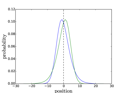
(a)

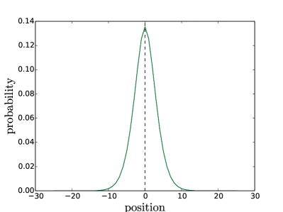
(b)

Figure 4: Probability distribution of the measurement in the standard basis and its reflection by the initial position for $t=20$ on the line segment of length 51, before procedure application Fig. 4(a) and after procedure application Fig. 4(b). In both cases we start in $\frac{1}{2}(|\tilde{v}_{0}^{0}\rangle\langle\tilde{v}_{0}^{0}|+|\tilde{v}_{0}^{1}\rangle\langle\tilde{v}_{0}^{1}|)$.

A further undesired effect has occurred for some symmetric graphs, where we observe the lack of symmetry of the probability distribution. Let us analyse the walk described in Eq. (22) on undirected segment graph. In Fig. 4(a) we present the probability distribution of the position measurement and the reflection of distribution according to the initial position. We observe that probability distribution is not symmetric with respect to the initial position.

Removing the locally rotating Hamiltonian doest not removed the asymmetry, hence it should come from the Lindbladian part of the evolution. Our analysis of transition rates suggests that such behaviour results from non-symmetry of the propagation $\tilde{\mathcal{M}}_{\tilde{v}\tilde{v}}^{\tilde{w}\tilde{z}}=\langle\tilde{w}|\tilde{L}|\tilde{v}\rangle\langle\tilde{v}|\tilde{L}^{\dagger}|\tilde{z}\rangle$. In the case of the Fourier matrix used in our model, values of $\tilde{\mathcal{M}}_{\tilde{v}\tilde{v}}^{\tilde{w}\tilde{z}}$ belong to a complex unit circle. Since the columns of matrices $A_{i}$, need to form an orthogonal basis, the values $\tilde{\mathcal{M}}_{\tilde{v}\tilde{v}}^{\tilde{w}\tilde{z}}$ will be different in general. We verified numerically, that there is no single matrix $A$, which can be used for all vertices of enlarged graph $\tilde{G}$ that removes the asymmetry. Hence we propose a different approach based on adding reflected operator.

Our idea is to add another global interaction Lindblad operator, with different $A_{i}$ matrices which will remove the side-effect. In the case of undirected segment, we choose $\tilde{\mathcal{L}}=\{\tilde{L}_{1},\tilde{L}_{2}\}$ with matrices $A_{i}^{(1)}$ and $A_{i}^{(2)}$ for the $i^{\textrm{th}}$ vertex. Henceforth, for $\tilde{L}_{1}$ we choose for each vertex

$$A_{i}^{(1)}=\begin{bmatrix}1&1\\ 1&-1\end{bmatrix}$$ (24)

and for $\tilde{L}_{2}$ we choose for each vertex

$$A_{i}^{(2)}=\begin{bmatrix}1&1\\ -1&1\end{bmatrix}.$$ (25)

Finally, the evolution takes the form

$$\frac{\textrm{d}}{\textrm{d}t}\tilde{\varrho}=-\mathrm{i}[\tilde{H}_{\textrm{rot}},\tilde{\varrho}]+\sum_{\tilde{L}\in\{\tilde{L}_{1},\tilde{L}_{2}\}}\left(\tilde{L}\tilde{\varrho}\tilde{L}^{\dagger}-\frac{1}{2}\{\tilde{L}^{\dagger}\tilde{L},\tilde{\varrho}\}\right).$$ (26)

Numerical analysis (see Fig. 4(b)) shows, that we obtain symmetric probability distribution for arbitrary time $t$. It is possible, that for the general graph the choice of different permutations of columns in $A_{i}$ matrix as $A_{i}^{(1)},A_{i}^{(2)},\ldots$ would suffice.

It is worth noting that for some graphs the symmetrization procedure is not necessary. For example, if we evolve quantum stochastic walks on undirected perfect $k$-ary tree, with the initial state localized in the root, we can observe that the distribution is symmetric due to arbitrary automorphism $A$ such that $A({\rm root})={\rm root}$. We have not found an explanation for this phenomenon yet.

4 The propagation speed and performance analysis

In [15] we have shown that quantum stochastic walk with the Hamiltonian operator and the global interaction Lindblad operator yields a ballistic propagation. However, because of the spontaneous moralization, the graph which was actually analysed was an undirected line with additional edges between every two vertices, see Fig. 5. Such observation does not diminish the results of [15], but gives additional incentive to recompute the scaling exponent of stochastic walks on a line by using new model. Hence, in this section we reproduce those results using our model, to verify if the fast propagation recorded in [15] for the global interaction case is due to the additional amplitude transitions or due to the quantum stochastic walk itself.

Figure 5: Line graph. Dashed lines correspond to additional amplitude transitions every two nodes coming from the GKSL model.

To do so we use the scaling exponent $\alpha$. We define it as a scaling parameter of the second moment $\mu_{2}(t)$, i.e.

$$\lim\limits_{t\to\infty}\frac{\mu_{2}(t)}{Ct^{\alpha}}=1$$ (27)

for some positive $C$ or equivalently

$$\mu_{2}(t)=\Theta\left(t^{\alpha}\right).$$ (28)

Generally, the greater the value of $\alpha$, the faster the walk propagates for large times. In the case of the walk on the line, it is well known that for the classical random walk we have $\alpha=1$ [18], and for the quantum walk $\alpha=2$ [13].

In [15] we have analysed evolution of the form

$$\frac{\mathrm{d}}{\mathrm{d}t}\varrho=-\mathrm{i}(1-\omega)[H,\varrho]+\omega\left(L\varrho L^{\dagger}-\frac{1}{2}\{L^{\dagger}L,\varrho\}\right),$$ (29)

where both $L$ and $H$ are adjacency matrix on the undirected line, and $\omega\in[0,1]$ is a free parameter of interaction strength. In [15] we demonstrated that for $\omega\in[0,1)$ the scaling exponent equals two, i.e. the propagation will follows the ballistic regime.

In our case, we consider the model based on the symmetrized quantum stochastic walk given by Eq. (26). We introduce a Hamiltonian, which is an adjacency matrix of the increased graph $\tilde{G}$, i.e.

$$\langle\tilde{i}|\tilde{H}|\tilde{j}\rangle=\begin{cases}1,&\langle\tilde{i}|\tilde{L}_{1}|\tilde{j}\rangle\neq 0,\\ 0,&\langle\tilde{i}|\tilde{L}_{1}|\tilde{j}\rangle=0,\end{cases}$$ (30)

The evolution takes the form

$$\begin{split}\frac{\textrm{d}}{\textrm{d}t}\tilde{\varrho}&=-\mathrm{i}(1-\omega)[\tilde{H},\tilde{\varrho}]+\omega\left(\mathrm{i}[\tilde{H}_{\textrm{rot}},\tilde{\varrho}]+\sum_{\tilde{L}\in\{\tilde{L}_{1},\tilde{L}_{2}\}}\left(\tilde{L}\tilde{\varrho}\tilde{L}^{\dagger}-\frac{1}{2}\{\tilde{L}^{\dagger}\tilde{L},\tilde{\varrho}\}\right)\right).\end{split}$$ (31)

In [15] we examined quantum stochastic walks on an undirected line. For the global interaction case we demonstrated that if $\omega\in[0,1)$, the scaling exponent equals two, and thus the propagation if ballistic. As it was shown in previous sections, in such case, the walk does not propagate on the line graph, but on the graph with additional edges between every two nodes, see Fig. 5. Such observation does no diminish the results of [15], but gives additional incentive to recompute the scaling exponent of stochastic walks on a line, by using our corrected model.

To determinate the scaling exponent we use a formula

$$\alpha=\lim_{t\to\infty}\frac{\log\mu_{2}(t)-\log C}{\log t}=\lim_{t\to\infty}\frac{\log\mu_{2}(t)}{\log t}.$$ (32)

First, we compute the second moment for $\omega\in\{0.5,0.6,0.7,0.8,0.9\}$ for different times from interval $[0,2400]$. Then, we chose 10 consecutive points and compute the linear regression of $\log(\mu_{2}(t))$ vs $\log(t)$. The slope of the regression approximates the scaling exponent. The result of numerical analysis is shown in Fig. 6.

We can see that for each value of $\omega$ the slope increases in time and exceeds $1$, which is the upper bound for classical propagation. The result suggests that, at least for some values of $\omega$, we have reproduced the ballistic propagation regime $\alpha\lesssim 2$. Moreover one can conclude, that the scaling exponent exceeds $1$ even for $\omega$ close to $1$.

Both results confirm that the fast propagation (ballistic or at least super-diffusive) is the property of global interaction case of the quantum stochastic walk and not from the fact that the original model allows additional transitions not according to the graph structure. Moreover, it confirms that our model preserves the super-diffusive propagation of the walk, at least for some interaction strength $\omega$.

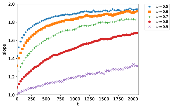
Figure 6: Slope of the local regression line for different values of $\omega$, respectively from top to bottom: $\omega=0.5,0.6,0.7,0.8,0.9$. We can see that for each value of the $\omega$ slope exceeds $1$ and increases in time.

The correction scheme presented in this paper enlarges the Hilbert space used. We can bound from above the dimension of constructed space. If the original graphs consists of $n$ vertices, with indegree indegree(v) for vertex $v$, then the size of enlarged Hilbert space equals $\sum_{v\in V}\textrm{indegree}(v)+\#\{v:\textrm{indegree}(v)=0\}$. If $\textrm{indegree}(v)=O(f(n))$ for all $v$, the size is roughly $nf(n)=O(n^{2})$ in the worst case scenario. In the term of number of qubits the additional qubit number is $O(\log n)$, hence in our opinion the correction scheme is efficient. Comparing to other models [taketani2016physical], where for each vertex there is corresponding qubit, size of our Hilbert space is still small. Moreover, while the correction can be applied to arbitrary digraph, real graphs are usually sparse, hence the indegree is much more smaller.

Furthermore, our corrections scheme preserves the geometry of the graph, since we do not create long range interactions: $\tilde{v}_{i}^{k}$ and $\tilde{v}_{j}^{k}$ are connected iff $v_{i}$ and $v_{j}$ or $v_{i}=v_{j}$. Hence from the geometry point of view, our model should not be much harder to realized than original global environment interaction case.

In our opinion an interesting further research direction would be generalization of our result onto multiplex networks, i.e. collection of graphs defined on the same vertex set. If Lindbladian operator would correspond to different graphs, quantum stochastic walks may have interesting new properties comparing to classical multiplex random walk. However, in order to define such an evolution, one need to generalize the correction scheme in order to remove spontaneous moralization on all Lindbladian operators at once.

5 Conclusions

In this paper we have shown, that the quantum stochastic walk global interaction case allows to transit amplitude not along the graph topology what makes a use of a global interaction case for a ranking algorithms impossible. We have discovered, that the graph, on which the evolution actually is made is the moral graph, hence we call this effect the spontaneous moralization. Furthermore we proposed a new model based on GKSL master equation with global Lindblad operator which do not posses such effect. We have recomputed the results from [15] in context of our model and we have confirmed that our corrections do not disturb the ballistic propagation of the walk. This demonstrates, the fast propagation corresponds not to classically forbidden transitions, but to the quantum stochastic walks model itself.

References

- [1] J. D. Whitfield, C. A. Rodríguez-Rosario, and A. Aspuru-Guzik, “Quantum stochastic walks: A generalization of classical random walks and quantum walks,” Physical Review A, vol. 81, no. 2, p. 022323, 2010.
- [2] A. Kossakowski, “On quantum statistical mechanics of non-hamiltonian systems,” Reports on Mathematical Physics, vol. 3, no. 4, pp. 247–274, 1972.
- [3] V. Gorini, A. Kossakowski, and E. C. G. Sudarshan, “Completely positive dynamical semigroups of n-level systems,” Journal of Mathematical Physics, vol. 17, no. 5, pp. 821–825, 1976.
- [4] G. Lindblad, “On the generators of quantum dynamical semigroups,” Communications in Mathematical Physics, vol. 48, no. 2, pp. 119–130, 1976.
- [5] P. E. Falloon, J. Rodriguez, and J. B. Wang, “Qswalk: a mathematica package for quantum stochastic walks on arbitrary graphs,” arXiv preprint arXiv:1606.04974, 2016.
- [6] S. Datta, “Electronic transport in mesoscopic systems (cambridge studies in semiconductor physics and microelectronic engineering),” Cambridge University Press, vol. 40, pp. 10011–4211, 1997.
- [7] V. Kendon, “Decoherence in quantum walks–a review,” Mathematical Structures in Computer Science, vol. 17, no. 06, pp. 1169–1220, 2007.
- [8] M. Mohseni, P. Rebentrost, S. Lloyd, and A. Aspuru-Guzik, “Environment-assisted quantum walks in photosynthetic energy transfer,” The Journal of chemical physics, vol. 129, no. 17, p. 174106, 2008.
- [9] R. E. Blankenship, Molecular mechanisms of photosynthesis. John Wiley & Sons, 2013.
- [10] E. Sánchez-Burillo, J. Duch, J. Gómez-Gardenes, and D. Zueco, “Quantum navigation and ranking in complex networks,” arXiv preprint arXiv:1202.3471, 2012.
- [11] T. Loke, J. Tang, J. Rodriguez, M. Small, and J. Wang, “Comparing classical and quantum pageranks,” arXiv preprint arXiv:1511.04823, 2015.
- [12] V. M. Kendon, “A random walk approach to quantum algorithms,” Philosophical Transactions of the Royal Society of London A: Mathematical, Physical and Engineering Sciences, vol. 364, no. 1849, pp. 3407–3422, 2006.
- [13] J. Kempe, “Quantum random walks: an introductory overview,” Contemporary Physics, vol. 44, no. 4, pp. 307–327, 2003.
- [14] H. Bringuier, “Central limit theorem and large deviation principle for continuous time open quantum walks,” arXiv preprint arXiv:1610.01298, 2016.
- [15] K. Domino, A. Glos, M. Ostaszewski, Ł. Pawela, and P. Sadowski, “Properties of quantum stochastic walks from the Hurst exponent,” arXiv preprint arXiv:1611.01349, 2016.
- [16] F. V. Jensen, An introduction to Bayesian networks, vol. 210. UCL press London, 1996.
- [17] J. A. Miszczak, “Singular value decomposition and matrix reorderings in quantum information theory,” International Journal of Modern Physics C, vol. 22, no. 09, pp. 897–918, 2011.
- [18] A. O. Caldeira and A. J. Leggett, “Path integral approach to quantum brownian motion,” Physica A: Statistical mechanics and its Applications, vol. 121, no. 3, pp. 587–616, 1983.