Direct and parametric synchronization of a graphene self-oscillator

Abstract

We explore the dynamics of a graphene nanomechanical oscillator coupled to a reference oscillator. Circular graphene drums are forced into self-oscillation, at a frequency $\mathrm{f_{osc}}$, by means of photothermal feedback induced by illuminating the drum with a continuous-wave red laser beam. Synchronization to a reference signal, at a frequency $\mathrm{f_{sync}}$, is achieved by shining a power-modulated blue laser onto the structure. We investigate two regimes of synchronization as a function of both detuning and signal strength for direct ($\mathrm{f_{sync}\approx f_{osc}}$) and parametric locking ($\mathrm{f_{sync}\approx 2f_{osc}}$). We detect a regime of phase resonance, where the phase of the oscillator behaves as an underdamped second-order system, with the natural frequency of the phase resonance showing a clear power-law dependence on the locking signal strength. The phase resonance is qualitatively reproduced using a forced van der Pol-Duffing-Mathieu equation.

Synchronization, also known as entrainment, is the phenomenon by which self-sustained oscillators mutually lock their frequencies and phase. Synchronization was first observed in a pair of coupled mechanical clocks by Huygens Huygens (1895); Oliveira and Melo (2015). Synchronized oscillators occur in a wide variety of engineered and biological systems such as injection-locked time keeping devices, the cardiac pacemaker cells and groups of fireflies Strogatz (2003); Matheny et al. (2014); Bagheri et al. (2013); Pikovsky et al. (2003). To study these phenomena experimentally, NanoElectroMechanical Systems (NEMS) have been proposed as representative model systems. Indeed, their strong nonlinearity, tunability, and convenient time scales make detailed experimental studies of synchronization possible, including the observation of features such as phase slipping, phase locking, phase inertia, and phase oscillation Cross et al. (2004); Shim et al. (2007); Zhang et al. (2012); Barois et al. (2014); Matheny et al. (2014). Compared to top-down fabricated NEMS devices, graphene nanomechanical systems offer enhanced nonlinear response due to their extreme aspect ratio. This enables new experimental studies of parametric synchronization and phase-oscillation dynamics, which are the topic of this Letter.
In this work we demonstrate synchronization of a single-layer graphene (SLG) nanomechanical oscillator to an optical reference signal. Two cases are considered: synchronization to a reference frequency close to the oscillator frequency, and close to twice the oscillator frequency. We investigate the synchronization dynamics for both cases and demonstrate the presence of phase oscillations, and show that their frequencies exhibit a distinct power-law dependence on the strength of the reference oscillator. The phase oscillations, are explained using a van der Pol-Duffing-Mathieu equation, and are shown to occur when the nonlinear spring constant of the oscillator exceeds a threshold value.
 The oscillator is fabricated by transferring a single layer of chemical vapor deposition (CVD) grown graphene onto an silicon substrate with circular cavities, which are etched into a 632 nm thick thermally grown silicon oxide layer. To reduce thermal drift, the graphene drum is placed in a cryogenic chamber with optical access (Montana Instruments), and cooled down to 3 K at a pressure of $\mathrm{<10^{-6}}$ mbar. Figure 1 shows the device and the setup. To induce self-oscillations, a red He-Ne laser ($\mathrm{\lambda}$ = 633 nm) is focused on the drum. The reflection from the silicon bottom of the cavity creates a partial standing wave which introduces a position-dependent thermally-induced mechanical tension in the structure Barton et al. (2012). The resulting photothermal force gradient, $\mathrm{\nabla F_{ph}}$, modifies the effective damping, given as $\mathrm{\Gamma_{eff}=\Gamma\left(1+\frac{\omega_{0}}{\Gamma}\frac{\omega_{0}\tau}{1+\omega^{2}\tau^{2}}\frac{\nabla F_{ph}}{\kappa}\right)}$ where, $\mathrm{\Gamma}$ ($\mathrm{\Gamma}={\omega_{0}}/{Q}$) is the damping without feedback , $\mathrm{\omega_{0}}$ and $\mathrm{\kappa}$ are the natural frequency and spring stiffness of the graphene drum, and $\mathrm{\tau}$ is the thermal delay time Metzger and Karrai (2004); Metzger et al. (2008). The thickness of the oxide layer is chosen as to maximize $\mathrm{\nabla F_{ph}}$. As a result, the effective damping becomes negative at low laser power, and the drum enters a regime of self-oscillation.
The membrane’s motion is detected using an interferometer as described in Refs. Bunch et al. (2007); Castellanos-Gomez et al. (2013). Briefly, a small portion of the incident red laser power is reflected off the graphene surface, and its interference with the light reflected from the silicon substrate underneath modulates the reflected intensity which is detected with a high-speed photodiode, as shown schematically in Fig. 1(a). The measurements are performed at an incident laser power of 10 mW. The motion of the graphene drum is recorded in the time-domain by sampling the photodiode output at 1 GS/s using an oscilloscope. At the same time, an external reference signal, to which the graphene drum oscillator will be locked, is provided by a blue laser diode (2.5 mW, $\mathrm{\lambda}$ = 405 nm) whose intensity is electronically modulated.
 Figure 1(b) shows the time-domain signals: the yellow trace indicates the free-running oscillator and the blue trace shows the output of the oscillator when the reference oscillator signal is applied. Figure 1(c) displays a zoom of the oscillations in more details. Figure 1(d) shows the power spectral densities (PSD) of the displacement signal, obtained by taking the FFT of the time traces. The spectral purity of the peak, given by its full-width at half-maximum (FWHM), is significantly better in the case the reference signal is applied (FWHM $\mathrm{<1}$ kHz) compared to the case without the reference signal (FWHM $\mathrm{\approx 35}$ kHz). While this is an indication that the SLG drum motion is locked to the reference oscillator, the PSD does not provide information regarding the phase coherence.

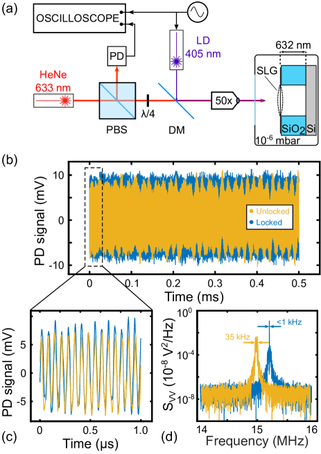
Figure 1: (a) Schematic representation of the measurement setup. A red He-Ne laser and a modulated blue laser are focused onto the drum via a window in the vacuum chamber of the cryostat at a temperature of 3 K. The displacement of the drum is detected using a photodiode (PD) and sampled with a digital oscilloscope. (b) A time-domain trace of the photodiode output for a free-running (yellow) and a synchronized (blue) oscillator. The frequency and power of the reference signal are $\mathrm{f_{sync}=15.19}$ MHz and a modulation strength of $\mathrm{P_{d}=1.5}$ mW respectively. (c) Zoom of the oscillation signal. (d) Power spectral density of the displacement and reference signals taken over a 1 ms time interval.

A more detailed picture of the oscillator phase is obtained by plotting the displacement signal on a slow (microseconds) and a fast (nanoseconds) time scale Strogatz (2003); Barois et al. (2014). Figure 2(a) shows such a plot for the freely running oscillator, where the phase diffuses after a few hundred microseconds Chen et al. (2013). In contrast, when the reference signal is applied (panel b) the phase is coherent during the measurement ($\mathrm{\sim}$1 ms). This demonstrates that the oscillator is synchronized to the reference signal. Interestingly, small phase fluctuations are noticeable on the slow time scale, which could indicate the presence of noise or higher order phase dynamics. These phase fluctuations become more apparent by plotting the in-phase component of the displacement versus its quadrature component with respect to the reference oscillator. The freely running oscillator Fig. 2(a) right panel shows a homogeneously distributed phase, while the locked oscillator phase (b, right panel) takes a fixed value. Note that a noise-free synchronized system would be represented by a single dot, significant fluctuations in both phase and amplitude are apparent in the synchronized graphene drum oscillator.
 To explain the dynamics of the synchronized oscillator in the presence of noise, we describe the system using the Adler equation Adler (1946); Paciorek (1965):

$$\mathrm{{\dot{\phi}}=-\frac{\mathrm{d}V(\phi)}{\mathrm{d}\phi}=-\Delta\omega+\gamma\sin(\frac{m}{n}\phi)+\xi(t)}.$$ (1)

Here $\mathrm{V(\phi)}$ is a periodic potential, $\mathrm{\phi}$ is the phase difference between the graphene oscillator and the reference signal, $\mathrm{\gamma}$ is the amplitude of the reference signal, $\mathrm{\Delta\omega}$ is the detuning between the oscillator’s natural frequency ($\mathrm{\omega_{osc}=2\pi f_{0}}$) and the reference signal ($\mathrm{\omega_{sync}=2\pi f_{sync}}$). $\mathrm{\xi(t)}$ is an additive stochastic term that represents the Brownian force noise. Synchronization occurs if $\mathrm{\Delta\omega=n\omega_{sync}-m\omega_{osc}}$, where m and n are integers. In the above experiment $\mathrm{m=n=1}$, which results in direct synchronization. In the following section we also consider the case where $\mathrm{m=2n=2}$, which results in a higher order (parametric) synchronization Adler (1946); Pikovsky et al. (2003).

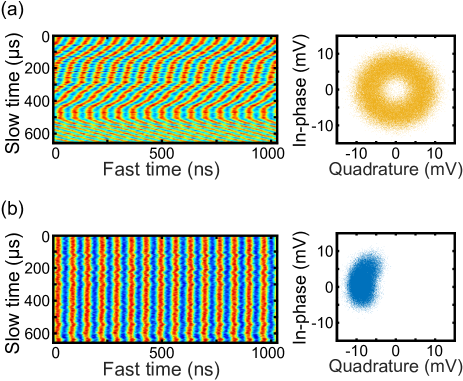
Figure 2: Raster plot (left panels) of the PD voltage of the free running (a) and locked (b) oscillators. The right panels show the corresponding I-Q plots.

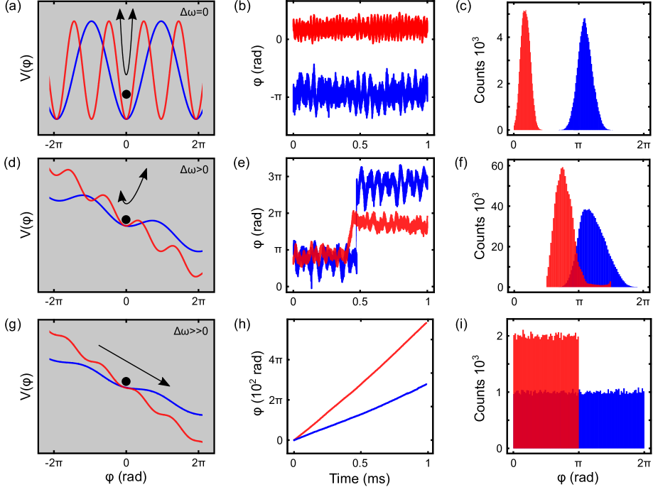
Figure 3: Washboard potential representation of entrainment, grey panels, for $\mathrm{\Delta\omega=0}$ (a), $\mathrm{\Delta\omega\approx 0}$ (d), and $\mathrm{\Delta\omega>0}$ (g). shown for the direct (blue) and parametric cases (red). (b) phase of the locked oscillator and the corresponding histogram (c). (e) noise-induced phase slips in a synchronized oscillator, and (f) the corresponding skewed-Gaussian distribution. Free-running phase of a unlocked oscillator (h) and the corresponding histogram showing a uniformly distributed phase (i).

Figure 3(a) shows the potential $\mathrm{V(\phi)}$ which has a period of $\mathrm{\frac{m}{n}2\pi}$. The blue curve represents the case where $\mathrm{f_{sync}=f_{osc}}$, while the red curve represents the parametric case with $\mathrm{f_{sync}=2f_{osc}}$. The phase of the oscillator is trapped in the potential minimum and fluctuates under the effect of noise. Figure 3(b) shows the experimentally obtained phase difference, as calculated by taking the Hilbert transform of the measured time trace for $\mathrm{\Delta\omega=0}$. Here the direct forcing frequency $\mathrm{f_{d}=15.19}$ MHz and the power $\mathrm{P_{d}=1.1}$ mW, while for the parametric case the forcing frequency $\mathrm{f_{p}=30.3}$ MHz and power $\mathrm{P_{p}=1.5}$ mW. A slight detuning, $\mathrm{\Delta\omega\neq 0}$, breaks the symmetry and causes the washboard potential to become tilted as shown schematically in Fig. 3(d) for $\mathrm{f_{d}=15.01}$ MHz, $\mathrm{P_{d}=0.75}$ mW, and $\mathrm{f_{p}=30.265}$ MHz, $\mathrm{P_{p}=0.35}$ mW. As the asymmetry created by tilting the potential reduces the barrier height, the system is now more prone to noise-induced phase slips where the phase undergoes a jump to the adjacent local minimum as the experimental data show in Fig. 3(e). Note that the direct forcing shows phase slips of $\mathrm{2\pi}$ whereas the parametric forcing shows phase slips of $\mathrm{\pi}$ as expected by theory. The asymmetry of the potential well is clearly reflected in the phase histograms. While a symmetric potential shows a Gaussian distribution Fig. 3(c), a tilted potential results in a skewed-Gaussian distribution Fig. 3(f). If the detuning is increased further, the tilt increases and the potential no longer represents a local minima, as shown in Fig. 3(g) for $\mathrm{f_{d}=14.78}$ MHz, $\mathrm{P_{d}=0.35}$ mW, and $\mathrm{f_{p}=30.01}$ MHz, $\mathrm{P_{p}=0.35}$ mW. The synchronization is lost, and the oscillator phase is free-running with respect to the reference signal, as shown in Fig. 3(h). In this case, the phase histogram is uniformly distributed over the $\mathrm{2\pi}$ and $\mathrm{\pi}$ range, Fig. 3(i).
One would naively expect to see no slow phase dynamics beyond locking. Interestingly, however, Fig. 3(b) shows that the phase in both direct and parametric cases oscillates with a period of $\mathrm{\sim 0.1}$ ms. These oscillations are known as phase inertia Barois et al. (2014). To extract the frequency of the phase oscillations, a Lorentzian function is fitted to the PSD of the phase, as shown in the inset in Fig. 4(a). By fitting the PSD for the different drive powers at zero detuning, the dependence of the phase oscillation frequency on synchronization signal strength is obtained. Figure 4(a) shows these plotted on a logarithmic scale for both direct (blue) an parametric (red) entrainment. The frequency of the phase oscillation shows a power-law dependence on the strength of the reference signals. The exponents are $\mathrm{S_{d}=0.56\pm 0.18}$ and $\mathrm{S_{p}=0.61\pm 0.03}$, as obtained from the fits in Fig. 4(a).

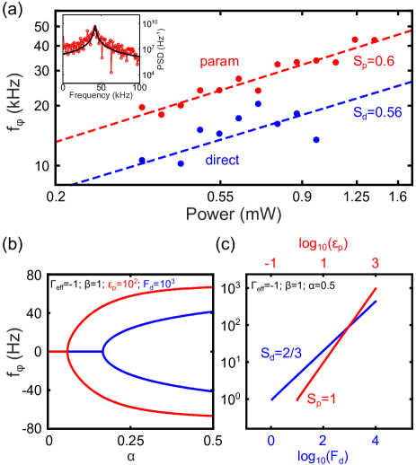
Figure 4: (a) Experimental power-law dependence of the phase resonance frequency on signal strength (rms signal power) for direct (blue) and parametric (red) locking. Inset shows a PSD of the phase and a Lorentzian fit. (b) Onset of phase oscillations as a function of $\mathrm{\pi}$ for direct (blue) and parametric (red) locking. (c) dependence of the phase oscillation frequency on direct (blue) and parametric (red) forcing. The parametric and direct cases present a linear and a sublinear dependence on forcing with $\mathrm{S_{d}=2/3}$ and $\mathrm{S_{p}=1}$

To capture the slow phase dynamics we model our system as a van der Pol oscillator with added terms to account for the Duffing nonlinearity, and the parametric and direct forcing Nayfeh and Mook (2008). The resulting forced van der Pol-Duffing-Mathieu equation expressed in non-dimensional form is given as :

$$\mathrm{\ddot{x}+(\Gamma_{eff}+\beta x^{2})\dot{x}+(1-\varepsilon_{p}\cos(\omega_{p}t))x+\alpha x^{3}=F_{d}\cos(\omega_{d}t)},$$ (2)

where the dot signifies taking the time-derivative, $\mathrm{x}$ is the normalized displacement, $\mathrm{\Gamma_{eff}}$ is the linear damping which in our case is negative due to photothermal feedback. $\mathrm{\beta}$ is a nonlinear damping term, $\mathrm{\varepsilon_{p}}$ is the strength of the parametric pumping term which is proportional to $\mathrm{P_{p}}$, $\mathrm{\omega_{p}}$ is the parametric pumping frequency, $\mathrm{\alpha}$ is the Duffing parameter, and $\mathrm{F_{d}}$ is the amplitude (proportional to $\mathrm{P_{d}}$) and $\mathrm{\omega_{d}}$ the frequency of the driving force. Note that for the cases studied in this work, the parametric forcing term $\mathrm{\varepsilon_{p}}$ and the direct forcing term $\mathrm{F_{d}}$ are never applied simultaneously.
The solution of Eq. (2) is expressed in terms of a slowly changing phase $\mathrm{\phi(t)}$ and amplitude $\mathrm{A(t)}$, by taking $\mathrm{x(t)=A(t)\cos(\omega t+\phi(t))}$ Balanov et al. (2008). Such solutions have been reported for the forced van der Pol-Duffing-Mathieu equation in Refs. Pandey et al. (2008); Belhaq and Fahsi (2008). For zero detuning, Eq. (2) can now be rewritten in terms of $\mathrm{\phi(t)}$ and $\mathrm{A(t)}$ as follows:

$$\begin{rcases}\mathrm{\dot{\phi}=-\frac{\varepsilon_{p}}{2A}\sin(2\phi)+\frac{F_{d}}{2A}\cos(\phi)+\frac{3}{8}{\alpha}\mid{A}\mid^{2}}\\ \mathrm{\dot{A}=-\frac{\Gamma_{eff}}{2}-\frac{\beta}{8}\mid{A}\mid^{2}A-\frac{\varepsilon_{p}}{2}\cos(2\phi)A-\frac{F_{d}}{2}\sin(\phi)}\\ \end{rcases}$$ (3)

Setting $\mathrm{\dot{\phi}=\dot{A}=0}$ gives the stationary solution ($\mathrm{A_{0}}$) as follows:

$$\mathrm{\left(\frac{9}{4}\bar{\alpha}^{2}+\frac{\beta}{16}\right)A^{6}_{0}+\frac{\Gamma_{eff}\beta}{2}A^{4}_{0}+(\Gamma_{eff}^{2}-\varepsilon_{p}^{2})A^{2}_{0}-{F_{d}^{2}}=0.}$$ (4)

To study the slow phase dynamics we use a perturbative approach, where we set $\mathrm{\phi}$ = $\mathrm{\phi_{0}}$ + $\mathrm{\hat{\phi}}$, and $\mathrm{A}$ = $\mathrm{A_{0}}$ + $\mathrm{\hat{A}}$, with the hats denoting a small deviation from stationary solution. By inserting these into Eq. (3), developing and keeping only first order terms, we obtain the following linear system of equations whose eigenvalues are the time constants of the phase oscillations:

$$\begin{rcases}\mathrm{\dot{\hat{\phi}}=-\left(\varepsilon_{p}\cos(2\phi_{0})+\frac{\Gamma_{eff}}{2}+\frac{1}{8}\beta A_{0}^{2}\right)\hat{\phi}-\left(\frac{3}{4}{\alpha}A_{0}+\frac{\varepsilon_{p}}{2A_{0}}\sin(2\phi_{0})\right)\hat{A}}\\ \mathrm{\dot{\hat{A}}=-\left(\varepsilon_{p}A_{0}\sin(2\phi_{0})+\frac{3}{4}\alpha A_{0}^{3}\right)\hat{\phi}+\left(\frac{\varepsilon_{p}}{2}\cos(2\phi_{0})-\frac{\Gamma_{eff}}{2}-\frac{3}{8}\beta A_{0}^{2}\right)\hat{A}}\\ \end{rcases}$$ (5)

The imaginary part of the eigenvalues of Eq. (5) gives the phase resonance frequency $\mathrm{f_{\phi}}$. These are obtained and plotted in Fig. 4(b) as a function of the Duffing parameters (for $\mathrm{\Gamma_{eff}=-1}$, $\mathrm{\beta=1}$, $\mathrm{\epsilon_{p}=10^{2}}$, and $\mathrm{F_{d}=10^{3}}$). For small $\mathrm{\alpha}$, the eigenvalues take only real values, indicating non-oscillatory, i.e. overdamped phase dynamics. As $\mathrm{\alpha}$ is increased, the eigenvalues become complex which indicates the transition to oscillatory phase behaviour. Figure 4(c) shows the dependence of the phase oscillation frequency on the synchronization signal strength for $\mathrm{\alpha}=0.5$. In the case of direct forcing (blue trace) the time constant shows a sublinear dependence on signal strength (slope = 2/3) while parametric forcing (red trace) exhibits a linear dependence (slope = 1). Remarkably, increasing $\mathrm{\alpha}$ or $\mathrm{\Gamma_{eff}}$ has no influence on these slopes. Thus, once phase oscillation sets in, its power-law exponent is independent of both nonlinearity and oscillation amplitude.
For $\mathrm{m=n=1}$, the experimentally obtained power-law dependence with $\mathrm{S_{d}=0.56}$ is in good agreement with the calculated $\mathrm{S_{d}=2/3}$. This is less the case for parametric synchronization, $\mathrm{m=2n=2}$, where the experimentally obtained value is $\mathrm{S_{p}=0.6}$ while in simulations $\mathrm{S_{p}=1}$. The discrepancy could indicate the presence of additional nonlinearity, which may originate from device asymmetry that is introduced, for instance, by wrinkles or a non-uniformly distributed residual strain Davidovikj et al. (2016). The demonstrated phase oscillations are expected to occur naturally in entrained graphene oscillators, since they are easily driven into the nonlinear regime Wang and Feng (2014), and their dependence on the drive strength and detuning with respect to the coupled reference oscillator may be used to further characterize the devices, or in applications that require the sensing of externally applied forces or masses Papariello et al. (2016).
In summary, the current work demonstrates that graphene self-oscillators can be synchronized to both a direct and parametric external signal at low temperatures. It is shown that achieving entrainment can significantly reduce the width of the oscillation peak, thus allowing reduction of oscillator frequency fluctuations to produce stable nanoscale oscillating motion. In addition to phase-locking and noise induced phase-slips, we also observed phase resonance and found that its frequency exhibits a power-law dependence on the drive signal strength for both direct and parametric synchronization. These oscillations were qualitatively reproduced using a forced van der Pol-Duffing-Mathieu equation, with the Duffing nonlinearity playing a crucial role in making such behaviour possible. This work enables synchronized motion of a large number of graphene oscillators, even if their resonance frequencies are slightly different. Potential applications of synchronized oscillators include optoelectronic modulators, sound generators and oscillating sensors.
 The authors acknowledge financial support from the European Union’s Seventh Framework Programme (FP7) under Grant Agreement $\mathrm{n{\circ}~{}318287}$, project LANDAUER. The research leading to these results has received funding from the European Union’s Horizon 2020 research and innovation program under Grant Agreement $\mathrm{n{\circ}~{}649953}$ (Graphene Flagship), and from the Dutch Technology Foundation STW Take-Off program, project $\mathrm{n{\circ}~{}14062}$.

References

- Huygens (1895) C. Huygens, Letters to de sluse,(letters; no. 1333 of 24 february 1665, no. 1335 of 26 february 1665, no. 1345 of 6 march 1665) (1895).
- Oliveira and Melo (2015) H. M. Oliveira and L. V. Melo, Scientific reports 5 (2015).
- Strogatz (2003) S. H. Strogatz, Sync: How order emerges from chaos in the universe, nature, and daily life (Hyperion, 2003).
- Matheny et al. (2014) M. H. Matheny, M. Grau, L. G. Villanueva, R. B. Karabalin, M. Cross, and M. L. Roukes, Physical review letters 112, 014101 (2014).
- Bagheri et al. (2013) M. Bagheri, M. Poot, L. Fan, F. Marquardt, and H. X. Tang, Physical review letters 111, 213902 (2013).
- Pikovsky et al. (2003) A. Pikovsky, M. Rosenblum, and J. Kurths, Synchronization: a universal concept in nonlinear sciences, vol. 12 (Cambridge university press, 2003).
- Cross et al. (2004) M. Cross, A. Zumdieck, R. Lifshitz, and J. Rogers, Physical review letters 93, 224101 (2004).
- Shim et al. (2007) S.-B. Shim, M. Imboden, and P. Mohanty, Science 316, 95 (2007).
- Zhang et al. (2012) M. Zhang, G. S. Wiederhecker, S. Manipatruni, A. Barnard, P. McEuen, and M. Lipson, Physical review letters 109, 233906 (2012).
- Barois et al. (2014) T. Barois, S. Perisanu, P. Vincent, S. T. Purcell, and A. Ayari, New Journal of Physics 16, 083009 (2014).
- Barton et al. (2012) R. A. Barton, I. R. Storch, V. P. Adiga, R. Sakakibara, B. R. Cipriany, B. Ilic, S. P. Wang, P. Ong, P. L. McEuen, J. M. Parpia, et al., Nano lett. 12, 4681 (2012).
- Metzger and Karrai (2004) C. H. Metzger and K. Karrai, Nature 432, 1002 (2004).
- Metzger et al. (2008) C. Metzger, I. Favero, A. Ortlieb, and K. Karrai, Phys. Rev. B 78, 035309 (2008).
- Bunch et al. (2007) J. S. Bunch, A. M. Van Der Zande, S. S. Verbridge, I. W. Frank, D. M. Tanenbaum, J. M. Parpia, H. G. Craighead, and P. L. McEuen, Science 315, 490 (2007).
- Castellanos-Gomez et al. (2013) A. Castellanos-Gomez, R. van Leeuwen, M. Buscema, H. S. van der Zant, G. A. Steele, and W. J. Venstra, Advanced Materials 25, 6719 (2013).
- Chen et al. (2013) C. Chen, S. Lee, V. V. Deshpande, G.-H. Lee, M. Lekas, K. Shepard, and J. Hone, Nat. nanotechnol. 8, 923 (2013).
- Adler (1946) R. Adler, Proceedings of the IRE 34, 351 (1946).
- Paciorek (1965) L. Paciorek, Proceedings of the IEEE 53, 1723 (1965).
- Nayfeh and Mook (2008) A. H. Nayfeh and D. T. Mook, Nonlinear oscillations (John Wiley & Sons, 2008).
- Balanov et al. (2008) A. Balanov, N. Janson, D. Postnov, and O. Sosnovtseva, Synchronization: from simple to complex (Springer Science & Business Media, 2008).
- Pandey et al. (2008) M. Pandey, R. H. Rand, and A. T. Zehnder, Nonlinear Dynamics 54, 3 (2008).
- Belhaq and Fahsi (2008) M. Belhaq and A. Fahsi, Nonlinear Dynamics 53, 139 (2008).
- Davidovikj et al. (2016) D. Davidovikj, J. J. Slim, S. J. Cartamil-Bueno, H. S. van der Zant, P. G. Steeneken, and W. J. Venstra, Nano letters 16, 2768 (2016).
- Wang and Feng (2014) Z. Wang and P. X.-L. Feng, Appl. Phys. Lett. 104, 103109 (2014).
- Papariello et al. (2016) L. Papariello, O. Zilberberg, A. Eichler, and R. Chitra, arXiv preprint arXiv:1603.07774 (2016).