The ${\Upsilon}(nS)$ ${\to}$ $B_{c}D_{s}$, $B_{c}D_{d}$ decays with perturbative QCD approach

Abstract

The ${\Upsilon}(nS)$ ${\to}$ $B_{c}D_{s}$, $B_{c}D_{d}$ weak decays are studied with the pQCD approach firstly. It is found that branching ratios ${\cal B}r({\Upsilon}(nS){\to}B_{c}D_{s})$ ${\sim}$ ${\cal O}(10^{-10})$ and ${\cal B}r({\Upsilon}(nS){\to}B_{c}D_{d})$ ${\sim}$ ${\cal O}(10^{-11})$, which might be measurable in the future experiments.

I Introduction

Since the discovery of bottomonium (the bound states of the bottom quark $b$ and the corresponding antiquark $\bar{b}$, i.e., $b\bar{b}$) at Fermilab in 1977 herb ; innes , remarkable achievements have been made in the understanding of the properties of bottomonium, thanks to the endeavor from the experiment groups of CLEO, BaBar, Belle, CDF, D0, LHCb, ATLAS, and so on 1212.6552 . The upsilon, ${\Upsilon}(nS)$, is the $S$-wave spin-triplet state, $n^{3}S_{1}$, of bottomonium with the well established quantum number of $I^{G}J^{PC}$ $=$ $0^{-}1^{--}$ pdg . The typical total widths of the upsilons below the kinematical open-bottom threshold (where the radial quantum number $n$ $=$ 1, 2 and 3) are a few tens of keV (see Table 1), at least two orders of magnitude lower less than those of bottomonium above the $B\bar{B}$ threshold. (note that for simplicity, the notation ${\Upsilon}(nS)$ will denote the ${\Upsilon}(1S)$, ${\Upsilon}(2S)$ and ${\Upsilon}(3S)$ mesons in the following content if not specified explicitly) As it is well known, the ${\Upsilon}(nS)$ meson decays primarily through the annihilation of the $b\bar{b}$ pairs into three gluons, which are suppressed by the phenomenological Okubo-Zweig-Iizuka rule o ; z ; i . The allowed $G$-parity conserving transitions, ${\Upsilon}(nS)$ ${\to}$ ${\pi}{\pi}{\Upsilon}(mS)$ and ${\Upsilon}(nS)$ ${\to}$ ${\eta}{\Upsilon}(mS)$ where $3$ $\geq$ $n$ $>$ $m$ ${\geq}$ $1$, are greatly limited by the compact phase spaces, because the mass difference $m_{{\Upsilon}(3S)}$ $-$ $m_{{\Upsilon}(2S)}$ is just slightly larger than $2m_{\pi}$, and $m_{{\Upsilon}(2S)}$ $-$ $m_{{\Upsilon}(1S)}$ is just slightly larger than $m_{\eta}$. The coupling strengths of the electromagnetic and radiative interactions are proportional to the electric charge of the bottom quark, $Q_{b}$ $=$ $-1/3$ in the unit of ${|}e{|}$. Besides, the ${\Upsilon}(nS)$ meson can also decay via the weak interactions within the standard model, although the branching ratio is small, about $2/{\tau}_{B}{\Gamma}_{{\Upsilon}}$ ${\sim}$ ${\cal O}(10^{-8})$ pdg , where ${\tau}_{B}$ and ${\Gamma}_{{\Upsilon}}$ are the lifetime of the $B_{u,d,s}$ meson and the total width of the ${\Upsilon}(nS)$ meson, respectively. In this paper, we will study the ${\Upsilon}(nS)$ ${\to}$ $B_{c}D_{s}$, $B_{c}D_{d}$ weak decays with the perturbative QCD (pQCD) approach pqcd1 ; pqcd2 ; pqcd3 . The motivation is listed as follows.

Table 1: Summary of the mass, total width and data samples of the ${\Upsilon}(1S,2S,3S)$ mesons.

	properties pdg		data samples ($10^{6}$) 1406.6311
meson	mass (MeV)	width (keV)	Belle	BaBar
${\Upsilon}(1S)$	$9460.30{\pm}0.26$	$54.02{\pm}1.25$	$102{\pm}2$	…
${\Upsilon}(2S)$	$10023.26{\pm}0.31$	$31.98{\pm}2.63$	$158{\pm}4$	$98.3{\pm}0.9$
${\Upsilon}(3S)$	$10355.2{\pm}0.5$	$20.32{\pm}1.85$	$11{\pm}0.3$	$121.3{\pm}1.2$

From the experimental point of view, (1) over $10^{8}$ ${\Upsilon}(nS)$ data samples have been accumulated by the Belle detector at the KEKB and the BaBar detector at the PEP-II $e^{+}e^{-}$ asymmetric energy colliders 1406.6311 (see Table 1). It is hopefully expected that more and more upsilons will be collected with great precision at the running upgraded LHC and the forthcoming SuperKEKB. An abundant data samples offer a realistic possibility to search for the ${\Upsilon}(nS)$ weak decays which in some cases might be detectable. (2) The signals for the ${\Upsilon}(nS)$ ${\to}$ $B_{c}D_{s,d}$ weak decays should be clear and easily distinguishable from background, because the back-to-back final states with opposite electric charges have definite momentums and energies in the center-of-mass frame of the ${\Upsilon}(nS)$ meson. In addition, the identification of either a single flavored $D_{s,d}$ or $B_{c}$ meson can be used not only to avoid the low double-tagging efficiency zpc62.271 , but also to provide an unambiguous evidence of the ${\Upsilon}(nS)$ weak decay. It should be noticed that on one hand, the ${\Upsilon}(nS)$ weak decays are very challenging to be observed experimentally due to their small branching ratios, on the other hand, any evidences of an abnormally large production rate of either a single charmed or bottomed meson might be a hint of new physics beyond the standard model zpc62.271 .

From the theoretical point of view, the ${\Upsilon}(nS)$ weak decays permit one to cross check parameters obtained from the $B$ meson decays, to further explore the underlying dynamical mechanism of the heavy quark weak decay, to test various theoretical approaches and to improve our understanding on the factorization properties. Phenomenologically, the ${\Upsilon}(nS)$ ${\to}$ $B_{c}D_{s}$, $B_{c}D_{d}$ weak decays are favored by the color factor due to the external $W$ emission topological structure, and by the Cabibbo-Kabayashi-Maskawa (CKM) elements ${|}V_{cb}{|}$ due to the $b$ ${\to}$ $c$ transition, so usually their branching ratio should not be too small. In addition, these two decay modes are the $U$-spin partners with each other, so the flavor symmetry breaking effects can be investigated. However, as far as we know, there is no study concerning on the ${\Upsilon}(nS)$ ${\to}$ $B_{c}D_{s,d}$ weak decays theoretically and experimentally at the moment. We wish this paper can provide a ready reference to the future experimental searches. Recently, many attractive methods have been fully developed to evaluate the hadronic matrix elements (HME) where the local quark-level operators are sandwiched between the initial and final hadron states, such as the pQCD approach pqcd1 ; pqcd2 ; pqcd3 , the QCD factorization qcdf1 ; qcdf2 ; qcdf3 and the soft and collinear effective theory scet1 ; scet2 ; scet3 ; scet4 , which could give an appropriate explanation for many measurements on the nonleptonic $B_{u,d}$ decays. In this paper, we will estimate the branching ratios for the ${\Upsilon}(nS)$ ${\to}$ $B_{c}D_{s,d}$ weak decays with the pQCD approach to offer a possibility of searching for these processes at the future experiments.

This paper is organized as follows. Section II is devoted to the theoretical framework and the amplitudes for the ${\Upsilon}(nS)$ ${\to}$ $B_{c}D_{s,d}$ decays. We present the numerical results and discussion in section III, and conclude with a summary in the last section.

II theoretical framework

II.1 The effective Hamiltonian

Using the operator product expansion and renormalization group equation, the effective Hamiltonian responsible for the ${\Upsilon}(nS)$ ${\to}$ $B_{c}D_{s,d}$ weak decays is written as 9512380

$${\cal H}_{\rm eff}\,=\,\frac{G_{F}}{\sqrt{2}}\,\sum\limits_{q=d,s}\Big{\{}V_{cb}V_{cp}^{\ast}\sum\limits_{i=1}^{2}C_{i}({\mu})\,Q_{i}^{q}({\mu})-V_{tb}V_{tp}^{\ast}\sum\limits_{j=3}^{10}C_{j}({\mu})\,Q_{j}^{q}({\mu})\Big{\}}+{\rm H.c.},$$ (1)

where $G_{F}$ $=$ $1.166{\times}10^{-5}\,{\rm GeV}^{-2}$ pdg is the Fermi coupling constant; the CKM factors are expressed as a power series in the Wolfenstein parameter ${\lambda}$ ${\sim}$ $0.2$ pdg ,

$$V_{cb}V_{cs}^{\ast} = +A{\lambda}^{2}-\frac{1}{2}A{\lambda}^{4}-\frac{1}{8}A{\lambda}^{6}(1+4A^{2})+{\cal O}({\lambda}^{7}),$$ (2)

$$V_{tb}V_{ts}^{\ast} = -V_{cb}V_{cs}^{\ast}-A{\lambda}^{4}({\rho}-i{\eta})+{\cal O}({\lambda}^{7}),$$ (3)

for the ${\Upsilon}(nS)$ ${\to}$ $B_{c}D_{s}$ decays, and

$$V_{cb}V_{cd}^{\ast} = -A{\lambda}^{3}+{\cal O}({\lambda}^{7}),$$ (4)

$$V_{tb}V_{td}^{\ast} = +A{\lambda}^{3}(1-{\rho}+i{\eta})+\frac{1}{2}A{\lambda}^{5}({\rho}-i{\eta})+{\cal O}({\lambda}^{7}).$$ (5)

for the ${\Upsilon}(nS)$ ${\to}$ $B_{c}D_{d}$ decays. The Wilson coefficients $C_{i}(\mu)$ summarize the physical contributions above the scale of ${\mu}$, and have been reliably calculated to the next-to-leading order with the renormalization group assisted perturbation theory. The local operators are defined as follows.

$$Q_{1}^{q} = [\bar{c}_{\alpha}{\gamma}_{\mu}(1-{\gamma}_{5})b_{\alpha}][\bar{q}_{\beta}{\gamma}^{\mu}(1-{\gamma}_{5})c_{\beta}],$$ (6)

$$Q_{2}^{q} = [\bar{c}_{\alpha}{\gamma}_{\mu}(1-{\gamma}_{5})b_{\beta}][\bar{q}_{\beta}{\gamma}^{\mu}(1-{\gamma}_{5})c_{\alpha}],$$ (7)

$$Q_{3}^{q} = \sum\limits_{q^{\prime}}[\bar{q}_{\alpha}{\gamma}_{\mu}(1-{\gamma}_{5})b_{\alpha}][\bar{q}^{\prime}_{\beta}{\gamma}^{\mu}(1-{\gamma}_{5})q^{\prime}_{\beta}],$$ (8)

$$Q_{4}^{q} = \sum\limits_{q^{\prime}}[\bar{q}_{\alpha}{\gamma}_{\mu}(1-{\gamma}_{5})b_{\beta}][\bar{q}^{\prime}_{\beta}{\gamma}^{\mu}(1-{\gamma}_{5})q^{\prime}_{\alpha}],$$ (9)

$$Q_{5}^{q} = \sum\limits_{q^{\prime}}[\bar{q}_{\alpha}{\gamma}_{\mu}(1-{\gamma}_{5})b_{\alpha}][\bar{q}^{\prime}_{\beta}{\gamma}^{\mu}(1+{\gamma}_{5})q^{\prime}_{\beta}],$$ (10)

$$Q_{6}^{q} = \sum\limits_{q^{\prime}}[\bar{q}_{\alpha}{\gamma}_{\mu}(1-{\gamma}_{5})b_{\beta}][\bar{q}^{\prime}_{\beta}{\gamma}^{\mu}(1+{\gamma}_{5})q^{\prime}_{\alpha}],$$ (11)

$$Q_{7}^{q} = \sum\limits_{q^{\prime}}\frac{3}{2}Q_{q^{\prime}}\,[\bar{q}_{\alpha}{\gamma}_{\mu}(1-{\gamma}_{5})b_{\alpha}][\bar{q}^{\prime}_{\beta}{\gamma}^{\mu}(1+{\gamma}_{5})q^{\prime}_{\beta}],$$ (12)

$$Q_{8}^{q} = \sum\limits_{q^{\prime}}\frac{3}{2}Q_{q^{\prime}}\,[\bar{q}_{\alpha}{\gamma}_{\mu}(1-{\gamma}_{5})b_{\beta}][\bar{q}^{\prime}_{\beta}{\gamma}^{\mu}(1+{\gamma}_{5})q^{\prime}_{\alpha}],$$ (13)

$$Q_{9}^{q} = \sum\limits_{q^{\prime}}\frac{3}{2}Q_{q^{\prime}}\,[\bar{q}_{\alpha}{\gamma}_{\mu}(1-{\gamma}_{5})b_{\alpha}][\bar{q}^{\prime}_{\beta}{\gamma}^{\mu}(1-{\gamma}_{5})q^{\prime}_{\beta}],$$ (14)

$$Q_{10}^{q} = \sum\limits_{q^{\prime}}\frac{3}{2}Q_{q^{\prime}}\,[\bar{q}_{\alpha}{\gamma}_{\mu}(1-{\gamma}_{5})b_{\beta}][\bar{q}^{\prime}_{\beta}{\gamma}^{\mu}(1-{\gamma}_{5})q^{\prime}_{\alpha}],$$ (15)

where $Q_{1,2}^{q}$, $Q_{3,{\cdots},6}^{q}$, and $Q_{7,{\cdots},10}^{q}$ are usually called as the tree operators, QCD penguin operators, and electroweak penguin operators, respectively; ${\alpha}$ and ${\beta}$ are color indices; $q^{\prime}$ denotes all the active quarks at the scale of ${\mu}$ ${\sim}$ ${\cal O}(m_{b})$, i.e., $q^{\prime}$ $=$ $u$, $d$, $s$, $c$, $b$; and $Q_{q^{\prime}}$ is the electric charge of the $q^{\prime}$ quark in the unit of ${|}e{|}$.

II.2 Hadronic matrix elements

Theoretically, to obtain the decay amplitudes, the remaining essential work and also the most complex part is the calculation of the hadronic matrix elements of local operators as accurate as possible. Combining the $k_{T}$ factorization theorem npb366 with the collinear factorization hypothesis, and based on the Lepage-Brodsky approach for exclusive processes prd22 , the HME can be written as the convolution of universal wave functions reflecting the nonperturbative contributions with hard scattering subamplitudes containing the perturbative contributions within the pQCD framework, where the transverse momentums of quarks are retained and the Sudakov factors are introduced, in order to regulate the endpoint singularities and provide a naturally dynamical cutoff on the nonperturbative contributions pqcd1 ; pqcd2 ; pqcd3 . Generally, the decay amplitude can be separated into three parts: the Wilson coefficients $C_{i}$ incorporating the hard contributions above the typical scale of $t$, the process-dependent scattering amplitudes $T$ accounting for the heavy quark decay, and the universal wave functions ${\Phi}$ including the soft and long-distance contributions, i.e.,

$${\int}dx\,db\,C_{i}(t)\,T(t,x,b)\,{\Phi}(x,b)e^{-S},$$ (16)

where $x$ is the longitudinal momentum fraction of valence quarks, $b$ is the conjugate variable of the transverse momentum $k_{T}$, and $e^{-S}$ is the Sudakov factor.

II.3 Kinematic variables

In the center-of-mass frame of the ${\Upsilon}(nS)$ mesons, the light cone kinematic variables are defined as follows.

$$p_{{\Upsilon}} = p_{1}\,=\,\frac{m_{1}}{\sqrt{2}}(1,1,0),$$ (17)

$$p_{B_{c}} = p_{2}\,=\,(p_{2}^{+},p_{2}^{-},0),$$ (18)

$$p_{D_{s,d}} = p_{3}\,=\,(p_{3}^{-},p_{3}^{+},0),$$ (19)

$$k_{i} = x_{i}\,p_{i}+(0,0,\vec{k}_{iT}),$$ (20)

$${\epsilon}_{\Upsilon}^{\parallel} = \frac{1}{\sqrt{2}}(1,-1,0),$$ (21)

$$p_{i}^{\pm} = (E_{i}\,{\pm}\,p)/\sqrt{2},$$ (22)

$$s = 2\,p_{2}{\cdot}p_{3},$$ (23)

$$t = 2\,p_{1}{\cdot}p_{2}=2\,m_{1}\,E_{2},$$ (24)

$$u = 2\,p_{1}{\cdot}p_{3}=2\,m_{1}\,E_{3},$$ (25)

$$p=\frac{\sqrt{[m_{1}^{2}-(m_{2}+m_{3})^{2}]\,[m_{1}^{2}-(m_{2}-m_{3})^{2}]}}{2\,m_{1}},$$ (26)

where $x_{i}$ is the longitudinal momentum fraction; $\vec{k}_{iT}$ is the transverse momentum; $p$ is the common momentum of final states; ${\epsilon}_{\Upsilon}^{\parallel}$ is the longitudinal polarization vector of the ${\Upsilon}(nS)$ meson; $m_{1}$ $=$ $m_{{\Upsilon}(nS)}$, $m_{2}$ $=$ $m_{B_{c}}$ and $m_{3}$ $=$ $m_{D_{s,d}}$ denote the masses of the ${\Upsilon}(nS)$, $B_{c}$ and $D_{s,d}$ mesons, respectively. The notation of momentum is displayed in Fig.2(a).

II.4 Wave functions

With the notation of Refs. jhep0605 ; jhep0703 , the HME of diquark operators squeezed between the vacuum and the ${\Upsilon}(nS)$, $B_{c}$, $D_{q}$ mesons are defined as follows.

$${\langle}0{|}b_{i}(z)\bar{b}_{j}(0){|}{\Upsilon}(p_{1},{\epsilon}_{\parallel}){\rangle}\,=\,\frac{1}{4}f_{\Upsilon}{\int}dk_{1}\,e^{-ik_{1}{\cdot}z}\Big{\{}\!\!\not{\epsilon}_{\parallel}\Big{[}m_{1}\,{\phi}_{\Upsilon}^{v}(k_{1})-\!\!\not{p}_{1}\,{\phi}_{\Upsilon}^{t}(k_{1})\Big{]}\Big{\}}_{ji},$$ (27)

$${\langle}B_{c}^{+}(p_{2}){|}\bar{c}_{i}(z)b_{j}(0){|}0{\rangle}\,=\,\frac{i}{4}f_{B_{c}}{\int}dk_{2}\,e^{ik_{2}{\cdot}z}\,\Big{\{}{\gamma}_{5}\Big{[}\!\!\not{p}_{2}\,{\phi}_{B_{c}}^{a}(k_{2})+m_{2}\,{\phi}_{B_{c}}^{p}(k_{2})\Big{]}\Big{\}}_{ji},$$ (28)

$${\langle}D_{q}^{-}(p_{3}){|}\bar{q}_{i}(z)c_{j}(0){|}0{\rangle}\ =\ \frac{i}{4}f_{D_{q}}{\int}_{0}^{1}dk_{3}\,e^{ik_{3}{\cdot}z}\Big{\{}{\gamma}_{5}\Big{[}\!\!\not{p}_{3}\,{\phi}_{D_{q}}^{a}(k_{3})+m_{3}\,{\phi}_{D_{q}}^{p}(k_{3})\Big{]}\Big{\}}_{ji},$$ (29)

where $f_{\Upsilon}$, $f_{B_{c}}$, $f_{D_{q}}$ are decay constants.

Because of the relations, $m_{{\Upsilon}(nS)}$ ${\simeq}$ $2m_{b}$, $m_{B_{c}}$ ${\simeq}$ $m_{b}$ $+$ $m_{c}$, and $m_{D_{q}}$ ${\simeq}$ $m_{c}$ $+$ $m_{q}$ (see Table 2), it might assume that the motion of the valence quarks in the considered mesons is nearly nonrelativistic. The wave functions of the ${\Upsilon}(nS)$, $B_{c}$, $D_{q}$ mesons could be approximately described with the nonrelativistic quantum chromodynamics prd46 ; prd51 ; rmp77 and Schrödinger equation. The wave functions of a nonrelativistic three-dimensional isotropic harmonic oscillator potential are given in Ref. plb751 ,

$${\phi}_{{\Upsilon}(1S)}^{v}(x)=A\,x\bar{x}\,{\exp}\Big{\{}-\frac{m_{b}^{2}}{8\,{\beta}_{1}^{2}\,x\,\bar{x}}\Big{\}},$$ (30)

$${\phi}_{{\Upsilon}(1S)}^{t}(x)=B\,(x-\bar{x})^{2}\,{\exp}\Big{\{}-\frac{m_{b}^{2}}{8\,{\beta}_{1}^{2}\,x\,\bar{x}}\Big{\}},$$ (31)

$${\phi}_{{\Upsilon}(2S)}^{t,v}(x)=C\,{\phi}_{{\Upsilon}(1S)}^{t,v}(x)\,\Big{\{}1+\frac{m_{b}^{2}}{2\,{\beta}_{1}^{2}\,x\,\bar{x}}\Big{\}},$$ (32)

$${\phi}_{{\Upsilon}(3S)}^{t,v}(x)=D\,{\phi}_{{\Upsilon}(1S)}^{t,v}(x)\,\Big{\{}\Big{(}1-\frac{m_{b}^{2}}{2\,{\beta}_{1}^{2}\,x\,\bar{x}}\Big{)}^{2}+6\Big{\}},$$ (33)

$${\phi}_{B_{c}}^{a}(x)=E\,x\bar{x}\,{\exp}\Big{\{}-\frac{\bar{x}\,m_{c}^{2}+x\,m_{b}^{2}}{8\,{\beta}_{2}^{2}\,x\,\bar{x}}\Big{\}},$$ (34)

$${\phi}_{B_{c}}^{p}(x)=F\,{\exp}\Big{\{}-\frac{\bar{x}\,m_{c}^{2}+x\,m_{b}^{2}}{8\,{\beta}_{2}^{2}\,x\,\bar{x}}\Big{\}},$$ (35)

$${\phi}_{D_{q}}^{a}(x)=G\,x\bar{x}\,{\exp}\Big{\{}-\frac{\bar{x}\,m_{q}^{2}+x\,m_{c}^{2}}{8\,{\beta}_{3}^{2}\,x\,\bar{x}}\Big{\}},$$ (36)

$${\phi}_{D_{q}}^{p}(x)=H\,{\exp}\Big{\{}-\frac{\bar{x}\,m_{q}^{2}+x\,m_{c}^{2}}{8\,{\beta}_{3}^{2}\,x\,\bar{x}}\Big{\}},$$ (37)

where ${\beta}_{i}$ $=$ ${\xi}_{i}{\alpha}_{s}({\xi}_{i})$ with ${\xi}_{i}$ $=$ $m_{i}/2$; parameters $A$, $B$, $C$, $D$, $E$, $F$, $G$, $H$ are the normalization coefficients satisfying the following conditions

$${\int}_{0}^{1}dx\,{\phi}_{{\Upsilon}(nS)}^{v,t}(x)=1,\quad{\int}_{0}^{1}dx\,{\phi}_{B_{c}}^{a,p}(x)=1,\quad{\int}_{0}^{1}dx\,{\phi}_{D_{q}}^{a,p}(x)=1.$$ (38)

The shape lines of the distribution amplitudes ${\phi}_{{\Upsilon}(nS)}^{v,t}(x)$ and ${\phi}_{B_{c}}^{a,p}(x)$ have been displayed in Ref. plb751 , which are basically consistent with the physical picture that the valence quarks share momentums according to their masses.

Here, one may question the nonrelativistic treatment on the wave functions of the $D_{s,d}$ mesons, because the motion of the light valence quark in $D$ meson is commonly assumed to be relativistic, and the behavior of the light valence quark in the heavy-light charmed $D_{s,d}$ mesons should be different from that in the heavy-heavy $B_{c}$ and ${\Upsilon}(nS)$ mesons. In addition, there are several phenomenological models for the $D_{s,d}$ meson wave functions, for example, Eq.(30) in Ref. prd78lv . The $D$ wave function, which is widely used within the pQCD framework, and is also favored by Ref. prd78lv via fitting with measurements on the $B$ ${\to}$ $DP$ decays, is written as

$${\phi}_{D}(x,b)=6\,x\bar{x}\,\Big{\{}1+C_{D}(1-2x)\Big{\}}{\exp}\Big{\{}-\frac{1}{2}w^{2}b^{2}\Big{\}},$$ (39)

where $C_{D}$ $=$ $0.5$ and $w$ $=$ $0.1$ GeV for the $D_{d}$ meson; $C_{D}$ $=$ $0.4$ and $w$ $=$ $0.2$ GeV for the $D_{s}$ meson; the exponential function represents the $k_{T}$ distribution. The same model of Eq.(39) is usually taken as the twist-2 and twist-3 distribution amplitudes in many practical applications prd78lv .

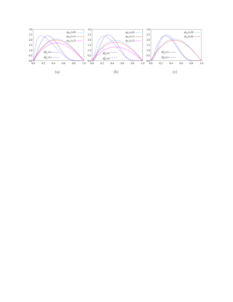
Figure 1: The distributions of the $D_{d}$ meson wave functions in (a), the distributions of the $D_{s}$ meson wave functions in (b), and the distributions of the $D_{s,d}$ meson wave functions in (c), where ${\phi}_{D_{q}}^{a}(x)$, ${\phi}_{D_{q}}^{p}(x)$, and ${\phi}_{D}(x,b)$ correspond to the Eq.(36), Eq.(37), and Eq.(39), respectively.

To show that the nonrelativistic description of the $D_{s,d}$ wave functions seems to be acceptable, the shape lines of the $D$ wave functions are displayed in Fig.1. It is clearly seen from Fig.1 that the shape lines of both Eq.(36) and Eq.(37) have a broad peak at the small $x$ regions, while the distributions of Eq.(39) is nearly symmetric to the variable $x$. This fact may imply that although the nonrelativistic model of the $D$ wave functions is crude, Eq.(36) and Eq.(37) can reflect, at least to some extent, the feature that the light valence quark might carry less momentums than the charm quark in the $D_{s,d}$ mesons. In addition, the flavor asymmetric effects, and the difference between the twist-2 and twist-3 distribution amplitudes are considered at least in part by Eq.(36) and Eq.(37). In the following calculation, we will use Eq.(36) and Eq.(37) as the twist-2 and twist-3 distribution amplitudes of the $D_{s,d}$ meson, respectively.

II.5 Decay amplitudes

The Feynman diagrams for the ${\Upsilon}(nS)$ ${\to}$ $B_{c}D_{s}$ decay are shown in Fig.2. There are two types: the emission and annihilation topologies, where diagram with gluon attaching to quarks in the same meson and between two different mesons are entitled factorizable and nonfactorizable diagrams, respectively.

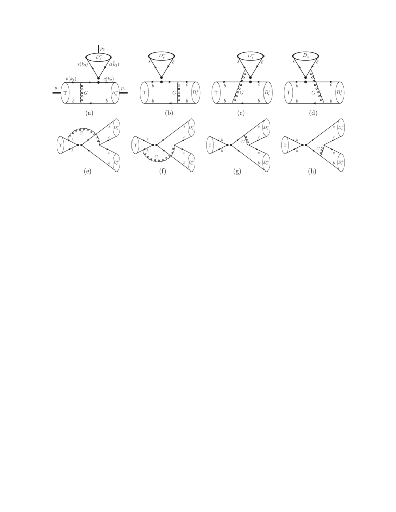
Figure 2: Feynman diagrams for the ${\Upsilon}(nS)$ ${\to}$ $B_{c}D_{s}$ decay with the pQCD approach, including the factorizable emission diagrams (a,b), the nonfactorizable emission diagrams (c,d), the nonfactorizable annihilation diagrams (e,f), and the factorizable annihilation diagrams (g,h).

By calculating these diagrams with the pQCD master formula Eq.(16), the decay amplitudes of ${\Upsilon}(nS)$ ${\to}$ $B_{c}D_{q}$ decays (where $q$ $=$ $d$, $s$) can be expressed as:

$${\cal A}({\Upsilon}(nS){\to}B_{c}D_{q})\ =\ \sqrt{2}\,G_{F}\,{\pi}\,f_{\Upsilon}\,f_{B_{c}}\,f_{D_{q}}\,\frac{C_{F}}{N}\,m_{{\Upsilon}}^{3}\,({\epsilon}_{\Upsilon}{\cdot}p_{D_{q}})$$ (40)

$${\times} \Big{\{}V_{cb}V_{cq}^{\ast}\,\Big{[}{\cal A}_{a+b}^{LL}\,a_{1}+{\cal A}_{c+d}^{LL}\,C_{2}\Big{]}-V_{tb}V_{tq}^{\ast}\,\Big{[}{\cal A}_{a+b}^{LL}\,(a_{4}+a_{10})$$

$$+{\cal A}_{a+b}^{SP}\,(a_{6}+a_{8})+{\cal A}_{c+d}^{LL}\,(C_{3}+C_{9})+{\cal A}_{c+d}^{SP}\,(C_{5}+C_{7})$$

$$+{\cal A}_{e+f}^{LL}\,(C_{3}+C_{4}-\frac{1}{2}C_{9}-\frac{1}{2}C_{10})+{\cal A}_{e+f}^{LR}\,(C_{6}-\frac{1}{2}C_{8})$$

$$+{\cal A}_{g+h}^{LL}\,(a_{3}+a_{4}-\frac{1}{2}a_{9}-\frac{1}{2}a_{10})+{\cal A}_{g+h}^{LR}\,(a_{5}-\frac{1}{2}a_{7})$$

$$+{\cal A}_{e+f}^{SP}\,(C_{5}-\frac{1}{2}C_{7})\Big{]}\Big{\}},$$

where $C_{F}$ $=$ $4/3$ and the color number $N$ $=$ $3$.

The parameters $a_{i}$ are defined as follows.

$$a_{i} = C_{i}+C_{i+1}/N,\quad(i=1,3,5,7,9);$$ (41)

$$a_{i} = C_{i}+C_{i-1}/N,\quad(i=2,4,5,6,10).$$ (42)

The building blocks ${\cal A}_{a+b}$, ${\cal A}_{c+d}$, ${\cal A}_{e+f}$, ${\cal A}_{g+h}$ denote the contributions of the factorizable emission diagrams Fig.2(a,b), the nonfactorizable emission diagrams Fig.2(c,d), the nonfactorizable annihilation diagrams Fig.2(e,f), the factorizable annihilation diagrams Fig.2(g,h), respectively. They are defined as

$${\cal A}_{i+j}^{k}={\cal A}_{i}^{k}+{\cal A}_{j}^{k},$$ (43)

where the subscripts $i$ and $j$ correspond to the indices of Fig.2; the superscript $k$ refers to one of the three possible Dirac structures, namely $k$ $=$ $LL$ for $(V-A){\otimes}(V-A)$, $k$ $=$ $LR$ for $(V-A){\otimes}(V+A)$, and $k$ $=$ $SP$ for $-2(S-P){\otimes}(S+P)$. The explicit expressions of these building blocks are collected in the Appendix A.

III Numerical results and discussion

In the rest frame of the ${\Upsilon}(nS)$ meson, the $CP$-averaged branching ratios for the ${\Upsilon}(nS)$ ${\to}$ $B_{c}D_{s,d}$ weak decays are written as

$${\cal B}r({\Upsilon}(nS){\to}B_{c}D_{s,d})\ =\ \frac{1}{12{\pi}}\,\frac{p}{m_{{\Upsilon}}^{2}{\Gamma}_{{\Upsilon}}}\,{|}{\cal A}({\Upsilon}(nS){\to}B_{c}D_{s,d}){|}^{2}.$$ (44)

Table 2: The numerical values of some input parameters.

The Wolfenstein parameters
$A$ $=$ $0.814^{+0.023}_{-0.024}$ pdg ,	${\lambda}$ $=$ $0.22537{\pm}0.00061$ pdg ,
$\bar{\rho}$ $=$ $0.117{\pm}0.021$ pdg ,	$\bar{\eta}$ $=$ $0.353{\pm}0.013$ pdg ,
Mass and decay constant
$m_{b}$ $=$ $4.78{\pm}0.06$ GeV pdg ,	$m_{c}$ $=$ $1.67{\pm}0.07$ GeV pdg ,
$m_{s}$ ${\simeq}$ $510$ MeV book ,	$m_{d}$ ${\simeq}$ $310$ MeV book ,
$m_{B_{c}}$ $=$ $6275.6{\pm}1.1$ MeV pdg ,	$m_{D_{s}}$ $=$ $1968.30{\pm}0.11$ MeV pdg ,
$m_{D_{d}}$ $=$ $1869.61{\pm}0.10$ MeV pdg ,
$f_{{\Upsilon}(1S)}$ $=$ $676.4{\pm}10.7$ MeV plb751	$f_{B_{c}}$ $=$ $489{\pm}5$ MeV fbc ,
$f_{{\Upsilon}(2S)}$ $=$ $473.0{\pm}23.7$ MeV plb751	$f_{D_{s}}$ $=$ $257.5{\pm}4.6$ MeV pdg ,
$f_{{\Upsilon}(3S)}$ $=$ $409.5{\pm}29.4$ MeV plb751	$f_{D_{d}}$ $=$ $204.6{\pm}5.0$ MeV pdg .

Table 3: The $CP$-averaged branching ratios for the ${\Upsilon}(nS)$ ${\to}$ $B_{c}D_{s,d}$ weak decays.

decay mode	${\cal B}r$
${\Upsilon}(1S)$ ${\to}$ $B_{c}D_{s}$	$(5.42^{+0.38+0.64+1.47}_{-0.37-0.60-0.76}){\times}10^{-10}$
${\Upsilon}(2S)$ ${\to}$ $B_{c}D_{s}$	$(4.28^{+0.30+0.49+0.93}_{-0.29-0.67-0.48}){\times}10^{-10}$
${\Upsilon}(3S)$ ${\to}$ $B_{c}D_{s}$	$(4.61^{+0.33+0.40+0.93}_{-0.31-0.88-0.52}){\times}10^{-10}$
${\Upsilon}(1S)$ ${\to}$ $B_{c}D_{d}$	$(1.96^{+0.15+0.23+0.56}_{-0.15-0.22-0.27}){\times}10^{-11}$
${\Upsilon}(2S)$ ${\to}$ $B_{c}D_{d}$	$(1.38^{+0.11+0.24+0.29}_{-0.10-0.05-0.15}){\times}10^{-11}$
${\Upsilon}(3S)$ ${\to}$ $B_{c}D_{d}$	$(1.58^{+0.12+0.15+0.33}_{-0.12-0.23-0.16}){\times}10^{-11}$

The input parameters are listed in Table 1 and 2. If not specified explicitly, we will take their central values as the default inputs. The numerical results on the $CP$-averaged branching ratios for the ${\Upsilon}(nS)$ ${\to}$ $B_{c}D_{s,d}$ weak decays are listed in Table 3, where the first uncertainties come from the CKM parameters; the second uncertainties are due to the variation of mass $m_{b}$ and $m_{c}$; the third uncertainties arise from the typical scale ${\mu}$ $=$ $(1{\pm}0.1)t_{i}$ and the expressions of $t_{i}$ for different topologies are given in Eqs.(77-80). The following are some comments.

(1) Because of the relation between the CKM factors ${|}V_{cb}V_{cs}^{\ast}{|}$ $>$ ${|}V_{cb}V_{cd}^{\ast}{|}$, and the relation between decay constants $f_{D_{s}}$ $>$ $f_{D_{d}}$, there is a hierarchical relation between branching ratios, i.e., ${\cal B}r({\Upsilon}(nS){\to}B_{c}D_{s})$ $>$ ${\cal B}r({\Upsilon}(nS){\to}B_{c}D_{d})$ for the same quantum number $n$.

(2) The relation among mass $m_{{\Upsilon}(3S)}$ $>$ $m_{{\Upsilon}(2S)}$ $>$ $m_{{\Upsilon}(1S)}$ and total width ${\Gamma}_{{\Upsilon}(3S)}$ $<$ ${\Gamma}_{{\Upsilon}(2S)}$ $<$ ${\Gamma}_{{\Upsilon}(1S)}$ should in principle result in the relation among branching ratios, ${\cal B}r({\Upsilon}(3S){\to}B_{c}D_{q})$ $>$ ${\cal B}r({\Upsilon}(2S){\to}B_{c}D_{q})$ $>$ ${\cal B}r({\Upsilon}(1S){\to}B_{c}D_{q})$. The numbers in Table 3 show that branching ratios for the ${\Upsilon}(nS)$ ${\to}$ $B_{c}D_{q})$ weak decays seem to be close to each other, and have almost nothing with the radial quantum number $n$. The reason may be that the decay amplitudes are proportional to decay constant $f_{{\Upsilon}(nS)}$, and hence there is an approximation,

$${\cal B}r({\Upsilon}(1S){\to}B_{c}D_{q}):{\cal B}r({\Upsilon}(2S){\to}B_{c}D_{q}):{\cal B}r({\Upsilon}(3S){\to}B_{c}D_{q})$$ (45)

$${\propto} \frac{f_{{\Upsilon}(1S)}^{2}}{{\Gamma}_{{\Upsilon}(1S)}}:\frac{f_{{\Upsilon}(2S)}^{2}}{{\Gamma}_{{\Upsilon}(2S)}}:\frac{f_{{\Upsilon}(3S)}^{2}}{{\Gamma}_{{\Upsilon}(3S)}}\ {\simeq}\ 1:1:1.$$

(3) Although different wave functions are used for the $D_{s,d}$ meson in the calculation due to the mass relation $m_{s}$ ${\neq}$ $m_{d}$ and $m_{D_{s}}$ ${\neq}$ $m_{D_{d}}$, the flavor symmetry breaking effects mainly appear in the CKM parameters and the decay constant $f_{D_{s,d}}$,

$$\frac{{\cal B}r({\Upsilon}(nS){\to}B_{c}D_{s})}{{\cal B}r({\Upsilon}(nS){\to}B_{c}D_{d})}\ {\simeq}\ \frac{{|}V_{cb}V_{cs}^{\ast}{|}^{2}\,f_{D_{s}}^{2}}{{|}V_{cb}V_{cd}^{\ast}{|}^{2}\,f_{D_{d}}^{2}},$$ (46)

for the same radial quantum number $n$.

(4) Compared the ${\Upsilon}(nS)$ ${\to}$ $B_{c}D_{s}$ decay with the ${\Upsilon}(nS)$ ${\to}$ $B_{c}{\pi}$ decay plb751 , they are both color-favored and CKM-favored. Only the emission topologies, and only the tree operators, contribute to the ${\Upsilon}(nS)$ ${\to}$ $B_{c}{\pi}$ decay, while both emission and annihilation topologies, and both tree and penguin operators, contribute to the ${\Upsilon}(nS)$ ${\to}$ $B_{c}D_{s}$ decay. In addition, the penguin contributions are dynamically enhanced due to the typical scale $t$ within the pQCD framework plb504 . These might explain the fact that although the final phase spaces for the ${\Upsilon}(nS)$ ${\to}$ $B_{c}D_{s}$ decay are more compact than those for the ${\Upsilon}(nS)$ ${\to}$ $B_{c}{\pi}$ decay, there is still the relation between branching ratios ${\cal B}r({\Upsilon}(nS){\to}B_{c}D_{s})$ $>$ ${\cal B}r({\Upsilon}(nS){\to}B_{c}{\pi})$.

(5) It is seen that branching ratios for the ${\Upsilon}(nS)$ ${\to}$ $B_{c}D_{s}$ ($B_{c}D_{d}$) decay can reach up to $10^{-10}$ ($10^{-11}$), which might be accessible at the running LHC and forthcoming SuperKEKB. For example, the ${\Upsilon}(nS)$ production cross section in p-Pb collision is a few ${\mu}b$ with the LHCb jhep1407 and ALICE plb740 detectors at LHC. Over $10^{12}$ ${\Upsilon}(nS)$ mesons per $ab^{-1}$ data collected at LHCb and ALICE are in principle available, corresponding to a few hundreds (tens) of the ${\Upsilon}(nS)$ ${\to}$ $B_{c}D_{s}$ ($B_{c}D_{d}$) events.

(6) Besides the uncertainties listed in Table 3, the decay constants can bring about 5%, 10%, 15% uncertainties to branching ratios for the ${\Upsilon}(1S)$ ${\Upsilon}(2S)$, ${\Upsilon}(3S)$ mesons decay into the $B_{c}D_{s,d}$ states, respectively, mainly from $f_{{\Upsilon}(2S,3S)}$. Other factors, such as the contributions of higher order corrections to HME, relativistic effects, different models for the wave functions, and so on, deserve the dedicated study. Our results just provide an order of magnitude estimation.

IV Summary

The ${\Upsilon}(nS)$ weak decay is allowable within the standard model, although the branching ratio is tiny and the experimental search is very difficult. With the potential prospects of the ${\Upsilon}(nS)$ at high-luminosity dedicated heavy-flavor factories, the ${\Upsilon}(nS)$ ${\to}$ $B_{c}D_{s,d}$ weak decays are studied with the pQCD approach firstly. It is found that with the nonrelativistic wave functions for ${\Upsilon}(nS)$, $B_{c}$, and $D_{s,d}$ mesons, branching ratios ${\cal B}r({\Upsilon}(nS){\to}B_{c}D_{s})$ ${\sim}$ ${\cal O}(10^{-10})$ and ${\cal B}r({\Upsilon}(nS){\to}B_{c}D_{d})$ ${\sim}$ ${\cal O}(10^{-11})$, which might be measurable in the future experiments.

Appendix A The building blocks of decay amplitudes

For the sake of simplicity, we decompose the decay amplitude Eq.(40) into some building blocks ${\cal A}_{i}^{k}$, where the subscript $i$ on ${\cal A}_{i}^{k}$ corresponds to the indices of Fig.2; the superscript $k$ on ${\cal A}_{i}^{k}$ refers to one of the three possible Dirac structures ${\Gamma}_{1}{\otimes}{\Gamma}_{2}$ of the four-quark operator $(\bar{q}_{1}{\Gamma}_{1}q_{2})(\bar{q}_{1}{\Gamma}_{2}q_{2})$, namely $k$ $=$ $LL$ for $(V-A){\otimes}(V-A)$, $k$ $=$ $LR$ for $(V-A){\otimes}(V+A)$, and $k$ $=$ $SP$ for $-2(S-P){\otimes}(S+P)$. The explicit expressions of ${\cal A}_{i}^{k}$ are written as follows.

$${\cal A}_{a}^{LL} = {\int}_{0}^{1}dx_{1}{\int}_{0}^{1}dx_{2}{\int}_{0}^{\infty}b_{1}db_{1}{\int}_{0}^{\infty}b_{2}db_{2}\,H_{a}({\alpha}_{e},{\beta}_{a},b_{1},b_{2})\,E_{a}(t_{a})$$ (47)

$${\alpha}_{s}(t_{a})\,{\phi}_{\Upsilon}^{v}(x_{1})\,\Big{\{}{\phi}_{B_{c}}^{a}(x_{2})\Big{[}x_{2}+r_{3}^{2}\,\bar{x}_{2}\Big{]}+{\phi}_{B_{c}}^{p}(x_{2})\,r_{2}\,r_{b}\Big{\}},$$

$${\cal A}_{a}^{SP} = -2\,r_{3}\,{\int}_{0}^{1}dx_{1}{\int}_{0}^{1}dx_{2}{\int}_{0}^{\infty}b_{1}db_{1}{\int}_{0}^{\infty}b_{2}db_{2}\,H_{a}({\alpha}_{e},{\beta}_{a},b_{1},b_{2})$$ (48)

$$E_{a}(t_{a})\,{\alpha}_{s}(t_{a})\,{\phi}_{\Upsilon}^{v}(x_{1})\,\Big{\{}{\phi}_{B_{c}}^{a}(x_{2})\,r_{b}+{\phi}_{B_{c}}^{p}(x_{2})\,r_{2}\,\bar{x}_{2}\Big{\}},$$

$${\cal A}_{b}^{LL} = {\int}_{0}^{1}dx_{1}{\int}_{0}^{1}dx_{2}{\int}_{0}^{\infty}b_{1}db_{1}{\int}_{0}^{\infty}b_{2}db_{2}\,H_{b}({\alpha}_{e},{\beta}_{b},b_{2},b_{1})\,E_{b}(t_{b})$$ (49)

$${\alpha}_{s}(t_{b})\,\Big{\{}{\phi}_{\Upsilon}^{v}(x_{1})\Big{[}2\,{\phi}_{B_{c}}^{p}(x_{2})\,r_{2}\,r_{c}-{\phi}_{B_{c}}^{a}(x_{2})\,(r_{2}^{2}\,x_{1}+r_{3}^{2}\,\bar{x}_{1})\Big{]}$$

$$+{\phi}_{\Upsilon}^{t}(x_{1})\Big{[}2\,{\phi}_{B_{c}}^{p}(x_{2})\,r_{2}\,x_{1}-{\phi}_{B_{c}}^{a}(x_{2})\,r_{c}\Big{]}\Big{\}},$$

$${\cal A}_{b}^{SP} = -2\,r_{3}\,{\int}_{0}^{1}dx_{1}{\int}_{0}^{1}dx_{2}{\int}_{0}^{\infty}b_{1}db_{1}{\int}_{0}^{\infty}b_{2}db_{2}\,H_{b}({\alpha}_{e},{\beta}_{b},b_{2},b_{1})$$ (50)

$$E_{b}(t_{b})\,{\alpha}_{s}(t_{b})\,\Big{\{}{\phi}_{\Upsilon}^{v}(x_{1})\Big{[}2\,{\phi}_{B_{c}}^{p}(x_{2})\,r_{2}-{\phi}_{B_{c}}^{a}(x_{2})\,r_{c}\Big{]}$$

$$-{\phi}_{\Upsilon}^{t}(x_{1})\,{\phi}_{B_{c}}^{a}(x_{2})\,\bar{x}_{1}\Big{\}},$$

$${\cal A}_{c}^{LL} = \frac{1}{N}{\int}_{0}^{1}dx_{1}{\int}_{0}^{1}dx_{2}{\int}_{0}^{1}dx_{3}{\int}_{0}^{\infty}db_{1}{\int}_{0}^{\infty}b_{2}db_{2}{\int}_{0}^{\infty}b_{3}db_{3}\,{\delta}(b_{1}-b_{2})\,{\alpha}_{s}(t_{c})$$ (51)

$$H_{cd}({\alpha}_{e},{\beta}_{c},b_{2},b_{3})\,E_{c}(t_{c})\,{\phi}_{D_{q}}^{a}(x_{3})\,\Big{\{}{\phi}_{\Upsilon}^{t}(x_{1})\,{\phi}_{B_{c}}^{p}(x_{2})\,r_{2}\,(x_{2}-x_{1})$$

$$+{\phi}_{\Upsilon}^{v}(x_{1})\,{\phi}_{B_{c}}^{a}(x_{2})\,\Big{[}\frac{s\,(x_{1}-\bar{x}_{3})}{m_{1}^{2}}\,+2\,r_{2}^{2}\,(x_{1}-x_{2})\Big{]}\Big{\}},$$

$${\cal A}_{c}^{SP} = -\frac{1}{N}\,r_{3}{\int}_{0}^{1}dx_{1}{\int}_{0}^{1}dx_{2}{\int}_{0}^{1}dx_{3}{\int}_{0}^{\infty}db_{1}{\int}_{0}^{\infty}b_{2}db_{2}{\int}_{0}^{\infty}b_{3}db_{3}\,{\delta}(b_{1}-b_{2})$$ (52)

$$H_{cd}({\alpha}_{e},{\beta}_{c},b_{2},b_{3})\,E_{c}(t_{c})\,{\alpha}_{s}(t_{c})\,{\phi}_{D_{q}}^{p}(x_{3})\,\Big{\{}{\phi}_{\Upsilon}^{t}(x_{1})\,{\phi}_{B_{c}}^{a}(x_{2})\,(x_{1}-\bar{x}_{3})$$

$$+{\phi}_{\Upsilon}^{v}(x_{1})\,{\phi}_{B_{c}}^{p}(x_{2})\,r_{2}\,(\bar{x}_{3}-x_{2})\Big{\}},$$

$${\cal A}_{d}^{LL} = \frac{1}{N}{\int}_{0}^{1}dx_{1}{\int}_{0}^{1}dx_{2}{\int}_{0}^{1}dx_{3}{\int}_{0}^{\infty}db_{1}{\int}_{0}^{\infty}b_{2}db_{2}{\int}_{0}^{\infty}b_{3}db_{3}\,{\delta}(b_{1}-b_{2})\,{\alpha}_{s}(t_{d})\,$$ (53)

$$H_{cd}({\alpha}_{e},{\beta}_{d},b_{2},b_{3})\,E_{d}(t_{d})\,\Big{\{}{\phi}_{\Upsilon}^{t}(x_{1})\,{\phi}_{B_{c}}^{p}(x_{2})\,{\phi}_{D_{q}}^{a}(x_{3})\,r_{2}\,(x_{2}-x_{1})$$

$$+{\phi}_{\Upsilon}^{v}(x_{1})\,{\phi}_{B_{c}}^{a}(x_{2})\,\Big{[}{\phi}_{D_{q}}^{a}(x_{3})\,\frac{s\,(x_{3}-x_{2})}{m_{1}^{2}}-{\phi}_{D_{q}}^{p}(x_{3})\,r_{3}\,r_{c}\Big{]}\Big{\}},$$

$${\cal A}_{d}^{SP} = -\frac{1}{N}\,r_{3}{\int}_{0}^{1}dx_{1}{\int}_{0}^{1}dx_{2}{\int}_{0}^{1}dx_{3}{\int}_{0}^{\infty}db_{1}{\int}_{0}^{\infty}b_{2}db_{2}{\int}_{0}^{\infty}b_{3}db_{3}\$$ (54)

$${\delta}(b_{1}-b_{2})\,H_{cd}({\alpha}_{e},{\beta}_{d},b_{2},b_{3})\,E_{d}(t_{d})\,{\alpha}_{s}(t_{d})\,$$

$$\Big{\{}{\phi}_{\Upsilon}^{v}(x_{1})\,{\phi}_{B_{c}}^{p}(x_{2})\,r_{2}\,\Big{[}{\phi}_{D_{q}}^{a}(x_{3})\,r_{c}/r_{3}+{\phi}_{D_{q}}^{p}(x_{3})\,(x_{2}-x_{3})\Big{]}$$

$$+{\phi}_{\Upsilon}^{t}(x_{1})\,{\phi}_{B_{c}}^{a}(x_{2})\,\Big{[}{\phi}_{D_{q}}^{p}(x_{3})\,(x_{3}-x_{1})-{\phi}_{D_{q}}^{a}(x_{3})\,r_{c}/r_{3}\Big{]}\Big{\}},$$

$${\cal A}_{e}^{LL} = \frac{1}{N}{\int}_{0}^{1}dx_{1}{\int}_{0}^{1}dx_{2}{\int}_{0}^{1}dx_{3}{\int}_{0}^{\infty}b_{1}db_{1}{\int}_{0}^{\infty}b_{2}db_{2}{\int}_{0}^{\infty}db_{3}\,{\delta}(b_{2}-b_{3})\,{\alpha}_{s}(t_{e})$$ (55)

$$H_{ef}({\alpha}_{a},{\beta}_{e},b_{1},b_{2})\,E_{e}(t_{e})\,\Big{\{}{\phi}_{\Upsilon}^{v}(x_{1})\Big{[}{\phi}_{B_{c}}^{p}(x_{2})\,{\phi}_{D_{q}}^{p}(x_{3})\,r_{2}\,r_{3}\,(x_{2}-\bar{x}_{3})$$

$$+{\phi}_{B_{c}}^{a}(x_{2})\,{\phi}_{D_{q}}^{a}(x_{3})\,\big{\{}\frac{s\,(x_{1}-\bar{x}_{3})}{m_{1}^{2}}+2\,r_{2}^{2}\,(x_{1}-x_{2})\big{\}}\Big{]}$$

$$-r_{b}\,{\phi}_{\Upsilon}^{t}(x_{1})\,{\phi}_{B_{c}}^{a}(x_{2})\,{\phi}_{D_{q}}^{a}(x_{3})\Big{\}},$$

$${\cal A}_{e}^{LR} = \frac{1}{N}{\int}_{0}^{1}dx_{1}{\int}_{0}^{1}dx_{2}{\int}_{0}^{1}dx_{3}{\int}_{0}^{\infty}b_{1}db_{1}{\int}_{0}^{\infty}b_{2}db_{2}{\int}_{0}^{\infty}db_{3}\,{\delta}(b_{2}-b_{3})\,{\alpha}_{s}(t_{e})$$ (56)

$$H_{ef}({\alpha}_{a},{\beta}_{e},b_{1},b_{2})\,E_{e}(t_{e})\,\Big{\{}{\phi}_{\Upsilon}^{v}(x_{1})\Big{[}{\phi}_{B_{c}}^{p}(x_{2})\,{\phi}_{D_{q}}^{p}(x_{3})\,r_{2}\,r_{3}\,(x_{2}-\bar{x}_{3})$$

$$+{\phi}_{B_{c}}^{a}(x_{2})\,{\phi}_{D_{q}}^{a}(x_{3})\,\big{\{}\frac{s\,(x_{2}-x_{1})}{m_{1}^{2}}+2\,r_{3}^{2}\,(\bar{x}_{3}-x_{1})\big{\}}$$

$$+r_{b}\,{\phi}_{\Upsilon}^{t}(x_{1})\,{\phi}_{B_{c}}^{a}(x_{2})\,{\phi}_{D_{q}}^{a}(x_{3})\Big{\}},$$

$${\cal A}_{e}^{SP} = \frac{1}{N}{\int}_{0}^{1}dx_{1}{\int}_{0}^{1}dx_{2}{\int}_{0}^{1}dx_{3}{\int}_{0}^{\infty}b_{1}db_{1}{\int}_{0}^{\infty}b_{2}db_{2}{\int}_{0}^{\infty}db_{3}\,{\delta}(b_{2}-b_{3})\,{\alpha}_{s}(t_{e})$$ (57)

$$H_{ef}({\alpha}_{a},{\beta}_{e},b_{1},b_{2})\,E_{e}(t_{e})\,\Big{\{}{\phi}_{\Upsilon}^{t}(x_{1})\Big{[}{\phi}_{B_{c}}^{a}(x_{2})\,{\phi}_{D_{q}}^{p}(x_{3})\,r_{3}\,(\bar{x}_{3}-x_{1})$$

$$+{\phi}_{B_{c}}^{p}(x_{2})\,{\phi}_{D_{q}}^{a}(x_{3})\,r_{2}\,(x_{2}-x_{1})\Big{]}+{\phi}_{\Upsilon}^{v}(x_{1})\,r_{b}\Big{[}{\phi}_{B_{c}}^{a}(x_{2})\,{\phi}_{D_{q}}^{p}(x_{3})\,r_{3}$$

$$+{\phi}_{B_{c}}^{p}(x_{2})\,{\phi}_{D_{q}}^{a}(x_{3})\,r_{2}\Big{]}\Big{\}},$$

$${\cal A}_{f}^{LL} = \frac{1}{N}{\int}_{0}^{1}dx_{1}{\int}_{0}^{1}dx_{2}{\int}_{0}^{1}dx_{3}{\int}_{0}^{\infty}b_{1}db_{1}{\int}_{0}^{\infty}b_{2}db_{2}{\int}_{0}^{\infty}db_{3}\,{\delta}(b_{2}-b_{3})\,{\alpha}_{s}(t_{f})$$ (58)

$$H_{ef}({\alpha}_{a},{\beta}_{e},b_{1},b_{2})\,E_{f}(t_{f})\,\Big{\{}{\phi}_{\Upsilon}^{v}(x_{1})\Big{[}{\phi}_{B_{c}}^{p}(x_{2})\,{\phi}_{D_{q}}^{p}(x_{3})\,r_{2}\,r_{3}\,(\bar{x}_{3}-x_{2})$$

$$+{\phi}_{B_{c}}^{a}(x_{2})\,{\phi}_{D_{q}}^{a}(x_{3})\,\{\frac{s\,(\bar{x}_{1}-x_{2})}{m_{1}^{2}}+2\,r_{3}^{2}\,(x_{3}-x_{1})\}\Big{]}$$

$$-r_{b}\,{\phi}_{\Upsilon}^{t}(x_{1})\,{\phi}_{B_{c}}^{a}(x_{2})\,{\phi}_{D_{q}}^{a}(x_{3})\Big{\}},$$

$${\cal A}_{f}^{LR} = \frac{1}{N}{\int}_{0}^{1}dx_{1}{\int}_{0}^{1}dx_{2}{\int}_{0}^{1}dx_{3}{\int}_{0}^{\infty}b_{1}db_{1}{\int}_{0}^{\infty}b_{2}db_{2}{\int}_{0}^{\infty}db_{3}\,{\delta}(b_{2}-b_{3})\,{\alpha}_{s}(t_{f})$$ (59)

$$H_{ef}({\alpha}_{a},{\beta}_{e},b_{1},b_{2})\,E_{f}(t_{f})\,\Big{\{}{\phi}_{\Upsilon}^{v}(x_{1})\Big{[}{\phi}_{B_{c}}^{p}(x_{2})\,{\phi}_{D_{q}}^{p}(x_{3})\,r_{2}\,r_{3}\,(\bar{x}_{3}-x_{2})$$

$$+{\phi}_{B_{c}}^{a}(x_{2})\,{\phi}_{D_{q}}^{a}(x_{3})\,\{\frac{s\,(x_{1}-x_{3})}{m_{1}^{2}}+2\,r_{2}^{2}\,(x_{2}-\bar{x}_{1})\}\Big{]}$$

$$+r_{b}\,{\phi}_{\Upsilon}^{t}(x_{1})\,{\phi}_{B_{c}}^{a}(x_{2})\,{\phi}_{D_{q}}^{a}(x_{3})\Big{\}},$$

$${\cal A}_{f}^{SP} = \frac{1}{N}{\int}_{0}^{1}dx_{1}{\int}_{0}^{1}dx_{2}{\int}_{0}^{1}dx_{3}{\int}_{0}^{\infty}b_{1}db_{1}{\int}_{0}^{\infty}b_{2}db_{2}{\int}_{0}^{\infty}db_{3}\,{\delta}(b_{2}-b_{3})\,{\alpha}_{s}(t_{f})$$ (60)

$$H_{ef}({\alpha}_{a},{\beta}_{e},b_{1},b_{2})\,E_{f}(t_{f})\,\Big{\{}{\phi}_{\Upsilon}^{t}(x_{1})\,\Big{[}{\phi}_{B_{c}}^{a}(x_{2})\,{\phi}_{D_{q}}^{p}(x_{3})\,r_{3}\,(x_{1}-x_{3})$$

$$+{\phi}_{B_{c}}^{p}(x_{2})\,{\phi}_{D_{q}}^{a}(x_{3})\,r_{2}\,(x_{2}-\bar{x}_{1})\Big{]}+{\phi}_{\Upsilon}^{v}(x_{1})\,r_{b}\,\Big{[}{\phi}_{B_{c}}^{a}(x_{2})\,{\phi}_{D_{q}}^{p}(x_{3})\,r_{3}$$

$$+{\phi}_{B_{c}}^{p}(x_{2})\,{\phi}_{D_{q}}^{a}(x_{3})\,r_{2}\Big{]}\Big{\}},$$

$${\cal A}_{g}^{LL} = {\cal A}_{g}^{LR}={\int}_{0}^{1}dx_{2}{\int}_{0}^{1}dx_{3}{\int}_{0}^{\infty}b_{2}db_{2}{\int}_{0}^{\infty}b_{3}db_{3}\,H_{gh}({\alpha}_{a},{\beta}_{g},b_{2},b_{3})\,E_{f}(t_{g})$$ (61)

$${\alpha}_{s}(t_{g})\,\Big{\{}{\phi}_{B_{c}}^{a}(x_{2})\,{\phi}_{D_{q}}^{a}(x_{3})\,(x_{2}+r_{3}^{2}\,\bar{x}_{2})-2\,{\phi}_{B_{c}}^{p}(x_{2})\,{\phi}_{D_{q}}^{p}(x_{3})\,r_{2}\,r_{3}\,\bar{x}_{2}\Big{\}},$$

$${\cal A}_{h}^{LL} = {\cal A}_{h}^{LR}={\int}_{0}^{1}dx_{2}{\int}_{0}^{1}dx_{3}{\int}_{0}^{\infty}b_{2}db_{2}{\int}_{0}^{\infty}b_{3}db_{3}\,H_{gh}({\alpha}_{a},{\beta}_{h},b_{3},b_{2})\,E_{h}(t_{h})$$ (62)

$${\alpha}_{s}(t_{h})\,\Big{\{}{\phi}_{B_{c}}^{a}(x_{2})\,{\phi}_{D_{q}}^{a}(x_{3})\,(\bar{x}_{3}+r_{2}^{2}\,x_{3})+{\phi}_{B_{c}}^{a}(x_{2})\,{\phi}_{D_{q}}^{p}(x_{3})\,r_{3}\,r_{b}$$

$$-2\,{\phi}_{B_{c}}^{p}(x_{2})\,{\phi}_{D_{q}}^{a}(x_{3})\,r_{2}\,r_{b}-2\,{\phi}_{B_{c}}^{p}(x_{2})\,{\phi}_{D_{q}}^{p}(x_{3})\,r_{2}\,r_{3}\,x_{3}\Big{\}},$$

where the mass ratio $r_{i}$ $=$ $m_{i}/m_{1}$; $\bar{x}_{i}$ $=$ $1$ $-$ $x_{i}$; variable $x_{i}$ is the longitudinal momentum fraction of the valence quark; $b_{i}$ is the conjugate variable of the transverse momentum $k_{i{\perp}}$; and ${\alpha}_{s}(t)$ is the QCD coupling at the scale of $t$.

The function $H_{i}$ are defined as follows.

$$H_{ab}({\alpha}_{e},{\beta},b_{i},b_{j}) = K_{0}(\sqrt{-{\alpha}_{e}}b_{i})\Big{\{}{\theta}(b_{i}-b_{j})K_{0}(\sqrt{-{\beta}}b_{i})I_{0}(\sqrt{-{\beta}}b_{j})+(b_{i}{\leftrightarrow}b_{j})\Big{\}},$$ (63)

$$H_{cd}({\alpha}_{e},{\beta},b_{2},b_{3}) = \Big{\{}{\theta}(-{\beta})K_{0}(\sqrt{-{\beta}}b_{3})+\frac{{\pi}}{2}{\theta}({\beta})\Big{[}iJ_{0}(\sqrt{{\beta}}b_{3})-Y_{0}(\sqrt{{\beta}}b_{3})\Big{]}\Big{\}}$$ (64)

$${\times} \Big{\{}{\theta}(b_{2}-b_{3})K_{0}(\sqrt{-{\alpha}_{e}}b_{2})I_{0}(\sqrt{-{\alpha}_{e}}b_{3})+(b_{2}{\leftrightarrow}b_{3})\Big{\}},$$

$$H_{ef}({\alpha}_{a},{\beta},b_{1},b_{2}) = \Big{\{}{\theta}(-{\beta})K_{0}(\sqrt{-{\beta}}b_{1})+\frac{{\pi}}{2}{\theta}({\beta})\Big{[}iJ_{0}(\sqrt{{\beta}}b_{1})-Y_{0}(\sqrt{{\beta}}b_{1})\Big{]}\Big{\}}$$ (65)

$$\!\!\!\!\!\!\!\!\!\!\!\!\!\!\!\!\!\!\!\!\!\!\!\!{\times}\frac{{\pi}}{2}\Big{\{}{\theta}(b_{1}-b_{2})\Big{[}iJ_{0}(\sqrt{{\alpha}_{a}}b_{1})-Y_{0}(\sqrt{{\alpha}_{a}}b_{1})\Big{]}J_{0}(\sqrt{{\alpha}_{a}}b_{2})+(b_{1}{\leftrightarrow}b_{2})\Big{\}},$$

$$H_{hg}({\alpha}_{a},{\beta},b_{i},b_{j}) = \frac{{\pi}^{2}}{4}\Big{\{}iJ_{0}(\sqrt{{\alpha}_{a}}b_{j})-Y_{0}(\sqrt{{\alpha}_{a}}b_{j})\Big{\}}$$ (66)

$${\times} \Big{\{}{\theta}(b_{i}-b_{j})\Big{[}iJ_{0}(\sqrt{{\beta}}b_{i})-Y_{0}(\sqrt{{\beta}}b_{i})\Big{]}J_{0}(\sqrt{{\beta}}b_{j})+(b_{i}{\leftrightarrow}b_{j})\Big{\}},$$

where $J_{0}$ and $Y_{0}$ ($I_{0}$ and $K_{0}$) are the (modified) Bessel functions of the first and second kind, respectively; ${\alpha}_{e}$ (${\alpha}_{a}$) is the gluon virtuality of the emission (annihilation) diagrams; the subscript of the quark virtuality ${\beta}_{i}$ corresponds to the indices of Fig.2. The definition of the particle virtuality is listed as follows.

$${\alpha}_{e} = \bar{x}_{1}^{2}m_{1}^{2}+\bar{x}_{2}^{2}m_{2}^{2}-\bar{x}_{1}\bar{x}_{2}t,$$ (67)

$${\alpha}_{a} = x_{2}^{2}m_{2}^{2}+\bar{x}_{3}^{2}m_{3}^{2}+x_{2}\bar{x}_{3}s,$$ (68)

$${\beta}_{a} = m_{1}^{2}-m_{b}^{2}+\bar{x}_{2}^{2}m_{2}^{2}-\bar{x}_{2}t,$$ (69)

$${\beta}_{b} = m_{2}^{2}-m_{c}^{2}+\bar{x}_{1}^{2}m_{1}^{2}-\bar{x}_{1}t,$$ (70)

$${\beta}_{c} = x_{1}^{2}m_{1}^{2}+x_{2}^{2}m_{2}^{2}+\bar{x}_{3}^{2}m_{3}^{2}$$ (71)

$$- x_{1}x_{2}t-x_{1}\bar{x}_{3}u+x_{2}\bar{x}_{3}s,$$

$${\beta}_{d} = x_{1}^{2}m_{1}^{2}+x_{2}^{2}m_{2}^{2}+x_{3}^{2}m_{3}^{2}-m_{c}^{2}$$ (72)

$$- x_{1}x_{2}t-x_{1}x_{3}u+x_{2}x_{3}s,$$

$${\beta}_{e} = x_{1}^{2}m_{1}^{2}+x_{2}^{2}m_{2}^{2}+\bar{x}_{3}^{2}m_{3}^{2}-m_{b}^{2}$$ (73)

$$- x_{1}x_{2}t-x_{1}\bar{x}_{3}u+x_{2}\bar{x}_{3}s,$$

$${\beta}_{f} = \bar{x}_{1}^{2}m_{1}^{2}+x_{2}^{2}m_{2}^{2}+\bar{x}_{3}^{2}m_{3}^{2}-m_{b}^{2}$$ (74)

$$- \bar{x}_{1}x_{2}t-\bar{x}_{1}\bar{x}_{3}u+x_{2}\bar{x}_{3}s,$$

$${\beta}_{g} = x_{2}^{2}m_{2}^{2}+m_{3}^{2}+x_{2}s,$$ (75)

$${\beta}_{h} = \bar{x}_{3}^{2}m_{3}^{2}+m_{2}^{2}+\bar{x}_{3}s-m_{b}^{2}.$$ (76)

The typical scale $t_{i}$ and the Sudakov factor $E_{i}$ are defined as follows, where the subscript $i$ corresponds to the indices of Fig.2.

$$t_{a(b)} = {\max}(\sqrt{-{\alpha}_{e}},\sqrt{-{\beta}_{a(b)}},1/b_{1},1/b_{2}),$$ (77)

$$t_{c(d)} = {\max}(\sqrt{-{\alpha}_{e}},\sqrt{{|}{\beta}_{c(d)}{|}},1/b_{2},1/b_{3}),$$ (78)

$$t_{e(f)} = {\max}(\sqrt{{\alpha}_{a}},\sqrt{{|}{\beta}_{e(f)}{|}},1/b_{1},1/b_{2}),$$ (79)

$$t_{g(h)} = {\max}(\sqrt{{\alpha}_{a}},\sqrt{{\beta}_{g(h)}},1/b_{2},1/b_{3}),$$ (80)

$$E_{i}(t)=\Bigg{\{}\begin{array}[]{lll}{\exp}\{-S_{B_{c}}(t)\},&{}&i=a,b\\ {\exp}\{-S_{B_{c}}(t)-S_{D_{q}}(t)\},&&i=c,d,e,f,g,h\end{array}$$ (81)

$$S_{B_{c}}(t) = s(x_{2},p_{2}^{+},1/b_{2})+2{\int}_{1/b_{2}}^{t}\frac{d{\mu}}{\mu}{\gamma}_{q},$$ (82)

$$S_{D_{q}}(t) = s(x_{3},p_{3}^{+},1/b_{3})+2{\int}_{1/b_{3}}^{t}\frac{d{\mu}}{\mu}{\gamma}_{q},$$ (83)

where ${\gamma}_{q}$ $=$ $-{\alpha}_{s}/{\pi}$ is the quark anomalous dimension; the explicit expression of $s(x,Q,1/b)$ can be found in the appendix of Ref.pqcd1 .

References

- (1) S. Herb et al., Phys. Rev. Lett. 39, 252 (1977).
- (2) W. Innes et al., Phys. Rev. Lett. 39, 1240 (1977).
- (3) C. Patrignani, T. Pedlar, and J. Rosner, Annu. Rev. Nucl. Part. Sci. 63, 21 (2013).
- (4) K. Olive et al. (Particle Data Group), Chin. Phys. C 38, 090001 (2014).
- (5) S. Okubo, Phys. Lett. 5, 165 (1963).
- (6) G. Zweig, CERN-TH-401, 402, 412 (1964).
- (7) J. Iizuka, Prog. Theor. Phys. Suppl. 37-38, 21 (1966).
- (8) H. Li, Phys. Rev. D 52, 3958 (1995).
- (9) C. Chang, H. Li, Phys. Rev. D 55, 5577 (1997).
- (10) T. Yeh, H. Li, Phys. Rev. D 56, 1615 (1997).
- (11) Ed. A. Bevan et al., Eur. Phys. J. C 74, 3026, (2014).
- (12) M. Sanchis-Lozano, Z. Phys. C 62, 271 (1994).
- (13) M. Beneke et al., Phys. Rev. Lett. 83, 1914 (1999).
- (14) M. Beneke et al., Nucl. Phys. B 591, 313 (2000).
- (15) M. Beneke et al., Nucl. Phys. B 606, 245 (2001).
- (16) C. Bauer et al., Phys. Rev. D 63, 114020 (2001).
- (17) C. Bauer, D. Pirjol, I. Stewart, Phys. Rev. D 65, 054022 (2002).
- (18) C. Bauer et al., Phys. Rev. D 66, 014017 (2002).
- (19) M. Beneke et al., Nucl. Phys. B 643, 431 (2002).
- (20) G. Buchalla, A. Buras, M. Lautenbacher, Rev. Mod. Phys. 68, 1125, (1996).
- (21) S. Catani, M. Ciafaloni, and F. Hautmann, Nucl. Phys. B 366, 135 (1991).
- (22) G. Lepage, S. Brodsky, Phys. Rev. D 22, 2157 (1980).
- (23) P. Ball, V. Braun, and A. Lenz, JHEP 0605, 004 (2006).
- (24) P. Ball, and G. Jones, JHEP 0703, 069 (2007).
- (25) G. Lepage et al., Phys. Rev. D 46, 4052 (1992).
- (26) G. Bodwin, E. Braaten, G. Lepage, Phys. Rev. D 51, 1125 (1995).
- (27) N. Brambilla et al., Rev. Mod. Phys. 77, 1423 (2005).
- (28) Y. Yang et al., Phys. Lett. B 751, 171 (2015).
- (29) R. Li, C. Lü, H. Zou, Phys. Rev. D 78, 014018 (2008).
- (30) A. Kamal, Particle physics, Springer, p.298 (2014).
- (31) T. Chiu, T. Hsieh, C. Huang, K. Ogawa, Phys. Lett. B 651, 171 (2007).
- (32) Y. Keum, H. Li, A. Sanda, Phys. Lett. B 504, 6 (2001).
- (33) R. Aaij et al. (LHCb Collaboration), JHEP 1407, 094 (2014).
- (34) B. Abelev et al. (ALICE Collaboration), Phys. Lett. B 740, 105 (2015).