Study of ${\Upsilon}(nS)$ ${\to}$ $B_{c}P$ decays with perturbative QCD approach

Abstract

With the potential prospects of the ${\Upsilon}(nS)$ at high-luminosity dedicated heavy-flavor factories, the color-favored ${\Upsilon}(nS)$ ${\to}$ $B_{c}{\pi}$, $B_{c}K$ weak decays are studied with the pQCD approach. It is found that branching ratios for the ${\Upsilon}(nS)$ ${\to}$ $B_{c}{\pi}$ decay are as large as the order of ${\cal O}(10^{-11})$, which might be measured promisingly by the future experiments.

I Introduction

Since the discovery of upsilons in proton-nucleus collisions at Fermilab in 1977 herb ; innes , remarkable achievements have been made in the understanding of the nature of bottomonium (bound state of $b\bar{b}$). The upsilon ${\Upsilon}(nS)$ is the spin-triplet $S$-wave state $n^{3}S_{1}$ of bottomonium with the well established quantum number of $I^{G}J^{PC}$ $=$ $0^{-}1^{--}$ pdg . The spectroscopy, production and decay mechanisms of the bottomonium resemble those of charmonium. The upsilon ${\Upsilon}(nS)$ below the $B\bar{B}$ threshold with the radial quantum number $n$ $=$ 1, 2 and 3 (note that for simplicity, the notation ${\Upsilon}(nS)$ will denote all ${\Upsilon}(1S)$, ${\Upsilon}(2S)$ and ${\Upsilon}(3S)$ mesons in the following content if not specified explicitly), in a close analogy with $J/{\psi}$, decay primarily through the annihilation of the $b\bar{b}$ pairs into three gluons, followed by the evolution of gluons into hadrons, glueballs, multiquark and other exotic states. The strong ${\Upsilon}(nS)$ decay offers an ideal plaza to glean the properties of the invisible gluons and of the quark-gluon coupling ann1983 . The ${\Upsilon}(nS)$ strong decays are suppressed by the Okubo-Zweig-Iizuka rules o ; z ; i , which enable electromagnetic and radiative transitions to become competitive. Besides, the upsilon weak decay is also legitimate within the standard model, although the branching ratio is tiny, about $2/{\tau}_{B}{\Gamma}_{\Upsilon}$ ${\sim}$ ${\cal O}(10^{-8})$ pdg . In this paper, we will estimate the branching ratios for the bottom-changing nonleptonic ${\Upsilon}(nS)$ ${\to}$ $B_{c}P$ weak decays with perturbative QCD (pQCD) approach pqcd1 ; pqcd2 ; pqcd3 , where $P$ denotes pseudoscalar ${\pi}$ and $K$ mesons. The motivation is listed as follows.

From the experimental point of view, (1) over $10^{8}$ ${\Upsilon}(nS)$ samples have been accumulated at Belle and Babar collaborations due to their outstanding performance 1406.6311 (see Table.1). It is hopefully expected that more than $10^{11}$ $b\bar{b}$ quark pairs would be available per $fb^{-1}$ data at LHCb 1408.0403 . Much more upsilons could be collected with great precision at the forthcoming SuperKEKB and the running upgraded LHC, which provide a golden opportunity to search for the ${\Upsilon}(nS)$ weak decays that in some cases might be detectable. Theoretical studies of the ${\Upsilon}(nS)$ weak decays are very necessary to offer a ready reference. (2) For the two-body ${\Upsilon}(nS)$ ${\to}$ $B_{c}{\pi}$, $B_{c}K$ decays, the back-to-back final states with opposite charges have definite energies and momenta in the center-of-mass frame of upsilons. Additionally, identification of a single flavored $B_{c}$ meson is free from inefficiently double tagging of flavored hadron pairs produced via conventional decays occurring above the $B\bar{B}$ threshold zpc62.271 , and can also provide a conclusive evidence of the upsilon weak decay. Of course, small branching ratios make the observation of the upsilon weak decays extremely challenging, and the observation of an abnormally large production rate of single $B_{c}$ mesons in the ${\Upsilon}(nS)$ decay might be a hint of new physics zpc62.271 .

Table 1: Summary of the mass, decay width and data samples of upsilon ${\Upsilon}(1S,2S,3S)$.

	properties pdg		data samples ($10^{6}$) 1406.6311
meson	mass (MeV)	width (keV)	Belle	BaBar
${\Upsilon}(1S)$	$9460.30{\pm}0.26$	$54.02{\pm}1.25$	$102{\pm}2$	…
${\Upsilon}(2S)$	$10023.26{\pm}0.31$	$31.98{\pm}2.63$	$158{\pm}4$	$98.3{\pm}0.9$
${\Upsilon}(3S)$	$10355.2{\pm}0.5$	$20.32{\pm}1.85$	$11{\pm}0.3$	$121.3{\pm}1.2$

From the theoretical point of view, the bottom-changing upsilon weak decays permit one to reexamine parameters obtained from $B$ meson decay, test various phenomenological models and improve our understanding on the strong interactions and the mechanism responsible for heavy meson weak decay. The ${\Upsilon}(nS)$ ${\to}$ $B_{c}P$ decays are monopolized by tree contributions and favored by the Cabibbo-Kobayashi-Maskawa (CKM) matrix element $V_{cb}$, so they should have relatively large branching ratios among nonleptonic upsilon weak decays. The ${\Upsilon}(1S)$ ${\to}$ $B_{c}{\pi}$, $B_{c}K$ decays have been studied with the naive factorization (NF) approximation in previous works zpc62.271 ; ijma14 ; adv2013 . One obvious deficiency of NF approach is the disappearance of strong phases and the renormalization scale from hadronic matrix elements (HME). Recently, several attractive methods have been developed to reevaluate HME, such as pQCD pqcd1 ; pqcd2 ; pqcd3 , the QCD factorization (QCDF) qcdf1 ; qcdf2 ; qcdf3 and soft and collinear effective theory scet1 ; scet2 ; scet3 ; scet4 . These methods have been widely used and could explain reasonably many measurements on nonleptonic $B_{u,d}$ decays. But, few works devote to the nonleptonic upsilon weak decays with these new phenomenological approaches. In this paper, we will study the ${\Upsilon}(nS)$ ${\to}$ $B_{c}{\pi}$, $B_{c}K$ weak decays with the pQCD approach.

This paper is organized as follows. In section II, we present the theoretical framework and the amplitudes for the ${\Upsilon}(nS)$ ${\to}$ $B_{c}{\pi}$, $B_{c}K$ decays with pQCD approach. Section III is devoted to numerical results and discussion. The last section is our summary.

II theoretical framework

II.1 The effective Hamiltonian

The effective Hamiltonian for the ${\Upsilon}(nS)$ ${\to}$ $B_{c}{\pi}$, $B_{c}K$ decays is written as 9512380

$${\cal H}_{\rm eff}\ =\ \frac{G_{F}}{\sqrt{2}}\,\sum\limits_{q=d,s}\,V_{cb}V_{uq}^{\ast}\,\Big{\{}C_{1}({\mu})\,Q_{1}({\mu})+C_{2}({\mu})\,Q_{2}({\mu})\Big{\}}+{\rm h.c.},$$ (1)

where $G_{F}$ is the Fermi coupling constant; the CKM factors are expanded as a power series in the small Wolfenstein parameter ${\lambda}$ ${\sim}$ 0.2 pdg ,

$$V_{cb}V_{ud}^{\ast} = A{\lambda}^{2}-\frac{1}{2}A{\lambda}^{4}-\frac{1}{8}A{\lambda}^{6}+{\cal O}({\lambda}^{8}),$$ (2)

$$V_{cb}V_{us}^{\ast} = A{\lambda}^{3}+{\cal O}({\lambda}^{8}).$$ (3)

The Wilson coefficients $C_{1,2}(\mu)$ summarize the physical contributions above scales of ${\mu}$, and have been properly calculated to the NLO order with the renormalization group improved perturbation theory. The local operators are defined as follows.

$$Q_{1} = [\bar{c}_{\alpha}{\gamma}_{\mu}(1-{\gamma}_{5})b_{\alpha}][\bar{q}_{\beta}{\gamma}^{\mu}(1-{\gamma}_{5})u_{\beta}],$$ (4)

$$Q_{2} = [\bar{c}_{\alpha}{\gamma}_{\mu}(1-{\gamma}_{5})b_{\beta}][\bar{q}_{\beta}{\gamma}^{\mu}(1-{\gamma}_{5})u_{\alpha}],$$ (5)

where ${\alpha}$ and ${\beta}$ are color indices and the sum over repeated indices is understood.

II.2 Hadronic matrix elements

To obtain the decay amplitudes, one has to calculate the hadronic matrix elements of local operators. Analogous to the common applications of hard exclusive processes in perturbative QCD proposed by Lepage and Brodsky prd22 , HME could be expressed as the convolution of hard scattering subamplitudes containing perturbative contributions with the universal wave functions reflecting the nonperturbative contributions. However, sometimes, the high-order corrections to HME produce collinear and/or soft logarithms based on collinear factorization approximation, for example, the spectator scattering amplitudes within the QCDF framework qcdf3 . The pQCD approach advocates that pqcd1 ; pqcd2 ; pqcd3 this problem could be settled down by retaining the transverse momentum of quarks and introducing the Sudakov factor. The decay amplitudes could be factorized into three parts: the soft effects uniting with the universal wave functions ${\Phi}$, the process-dependent subamplitude $H$, the hard effects incorporated into the Wilson coefficients $C_{i}$. For a particular topology, the decay amplitudes could be written as

$${\cal A}_{i}\ {\propto}\ \prod\limits_{j}{\int}dx_{j}\,db_{j}\,C_{i}(t)\,H_{i}(t_{i},x_{j},b_{j})\,{\Phi}_{j}(x_{j},b_{j})\,e^{-S},$$ (6)

where $t_{i}$ is a typical scale, $x_{j}$ is the longitudinal momentum fraction of the valence quark, $b_{j}$ is the conjugate variable of the transverse momentum, $e^{-S}$ is the Sudakov factor, and $j$ denotes participating particles.

II.3 Kinematic variables

In the ${\Upsilon}(nS)$ rest frame, the light cone kinematic variables are defined as

$$p_{{\Upsilon}}\,=\,p_{1}\,=\,\frac{m_{1}}{\sqrt{2}}(1,1,0),$$ (7)

$$p_{B_{c}}\,=\,p_{2}\,=\,(p_{2}^{+},p_{2}^{-},0),$$ (8)

$$p_{\pi(K)}\,=\,p_{3}\,=\,(p_{3}^{-},p_{3}^{+},0),$$ (9)

$$k_{i}\,=\,x_{i}\,p_{i}+(0,0,\vec{k}_{i{\perp}}),$$ (10)

$${\epsilon}_{\Upsilon}^{\parallel}\,=\,\frac{1}{\sqrt{2}}(1,-1,0),$$ (11)

$$n_{+}=(1,0,0),\quad n_{-}=(0,1,0),$$ (12)

$$p_{i}^{\pm}\,=\,\frac{E_{i}\,{\pm}\,p}{\sqrt{2}},$$ (13)

$$p\,=\,\frac{\sqrt{[m_{1}^{2}-(m_{2}+m_{3})^{2}][m_{1}^{2}-(m_{2}-m_{3})^{2}]}}{2\,m_{1}},$$ (14)

$$s\,=\,2\,p_{2}{\cdot}p_{3}\,=\,m_{1}^{2}-m_{2}^{2}-m_{3}^{2},$$ (15)

$$t\,=\,2\,p_{1}{\cdot}p_{2}\,=\,m_{1}^{2}+m_{2}^{2}-m_{3}^{2}\,=\,2\,m_{1}\,E_{2},$$ (16)

$$u\,=\,2\,p_{1}{\cdot}p_{3}\,=\,m_{1}^{2}-m_{2}^{2}+m_{3}^{2}\,=\,2\,m_{1}\,E_{3},$$ (17)

$$t+u-s\,=\,m_{1}^{2}+m_{2}^{2}+m_{3}^{2},$$ (18)

where $x_{i}$ and $\vec{k}_{i{\perp}}$ are the longitudinal momentum fraction and transverse momentum of the light valence quark, respectively; ${\epsilon}_{\Upsilon}^{\parallel}$ is the longitudinal polarization vector of the ${\Upsilon}(nS)$ particle; $n_{+}$ and $n_{-}$ are positive and negative null vectors, respectively; $p$ is the common momentum of final states; $m_{1}$, $m_{2}$ and $m_{3}$ denote the masses of the ${\Upsilon}(nS)$, $B_{c}$ and ${\pi}(K)$ mesons, respectively. The notation of momentum is displayed in Fig.2(a).

II.4 Wave functions

With the notation in prd65.014007 ; npb529.323 ; jhep0605.004 , the definitions of matrix elements of diquark operators sandwiched between vacuum and the longitudinally polarized ${\Upsilon}(nS)$, the double-heavy pseudoscalar $B_{c}$, the light pseudoscalar $P$ are

$${\langle}0{|}b_{i}(z)\bar{b}_{j}(0){|}{\Upsilon}(p_{1},{\epsilon}_{\parallel}){\rangle}\,=\,\frac{1}{4}f_{\Upsilon}{\int}dx_{1}\,e^{-ix_{1}p_{1}{\cdot}z}\Big{\{}\!\!\not{\epsilon}_{\parallel}\Big{[}m_{1}\,{\phi}_{\Upsilon}^{v}(x_{1})-\!\!\not{p}_{1}\,{\phi}_{\Upsilon}^{t}(x_{1})\Big{]}\Big{\}}_{ji},$$ (19)

$${\langle}B_{c}^{+}(p_{2}){|}\bar{c}_{i}(z)b_{j}(0){|}0{\rangle}\,=\,\frac{i}{4}f_{B_{c}}{\int}dx_{2}\,e^{ix_{2}p_{2}{\cdot}z}\,\Big{\{}{\gamma}_{5}\Big{[}\!\!\not{p}_{2}\,{\phi}_{B_{c}}^{a}(x_{2})+m_{2}\,{\phi}_{B_{c}}^{p}(x_{2})\Big{]}\Big{\}}_{ji},$$ (20)

$${\langle}P(p_{3}){|}u_{i}(z)\bar{q}_{j}(0){|}0{\rangle}$$ (21)

$$= \frac{i}{4}f_{P}{\int}dx_{3}\,e^{ix_{3}p_{3}{\cdot}z}\Big{\{}{\gamma}_{5}\Big{[}\!\!\not{p}_{3}\,{\phi}_{P}^{a}(x_{3})+{\mu}_{P}{\phi}_{P}^{p}(x_{3})-{\mu}_{P}(\!\not{n}_{-}\!\!\not{n}_{+}\!-\!1)\,{\phi}_{P}^{t}(x_{3})\Big{]}\Big{\}}_{ji},$$

where $f_{\Upsilon}$, $f_{B_{c}}$, $f_{P}$ are decay constants, ${\mu}_{P}$ $=$ $m_{3}^{2}/(m_{u}+m_{q})$ and $q$ $=$ $d(s)$ for ${\pi}(K)$ meson.

The twist-2 distribution amplitudes of light pseudoscalar ${\pi}$, $K$ mesons are defined as jhep0605.004 :

$${\phi}_{P}^{a}(x)=6\,x\bar{x}\Big{\{}1+\sum\limits_{n=1}^{\infty}a_{n}^{P}\,C_{n}^{3/2}(x-\bar{x})\Big{\}},$$ (22)

where $\bar{x}$ $=$ $1$ $-$ $x$; $a_{n}^{P}$ and $C_{n}^{3/2}(z)$ are Gegenbauer moment and polynomials, respectively; $a^{\pi}_{i}$ $=$ $0$ for $i$ $=$ 1, 3, 5, ${\cdots}$ due to the explicit $G$-parity of pion.

Both ${\Upsilon}(nS)$ and $B_{c}$ systems are nearly nonrelativistic, due to $m_{{\Upsilon}}$ ${\simeq}$ $2m_{b}$ and $m_{B_{c}}$ ${\simeq}$ $m_{b}$ $+$ $m_{c}$. Nonrelativistic quantum chromodynamics (NRQCD) prd46 ; prd51 ; rmp77 and Schrödinger equation can be used to describe their spectrum. The radial wave functions with isotropic harmonic oscillator potential are written as

$${\phi}_{1S}(\vec{k})\ {\sim}\ e^{-\vec{k}^{2}/2{\beta}^{2}},$$ (23)

$${\phi}_{2S}(\vec{k})\ {\sim}\ e^{-\vec{k}^{2}/2{\beta}^{2}}(2\vec{k}^{2}-3{\beta}^{2}),$$ (24)

$${\phi}_{3S}(\vec{k})\ {\sim}\ e^{-\vec{k}^{2}/2{\beta}^{2}}(4\vec{k}^{4}-20\vec{k}^{2}{\beta}^{2}+15{\beta}^{4}),$$ (25)

where the parameter ${\beta}$ determines the average transverse momentum, i.e., ${\langle}1S{|}\vec{k}^{2}_{\perp}{|}1S{\rangle}$ $=$ ${\beta}^{2}$. According to the NRQCD power counting rules prd46 , the characteristic magnitude of the momentum of heavy quark is order of $Mv$, where $M$ is the mass of the heavy quark with typical velocity $v$ ${\sim}$ ${\alpha}_{s}(M)$. So, value of ${\beta}$ $=$ $M{\alpha}_{s}(M)$ is taken in our calculation. Employing the substitution ansatz xiao ,

$$\vec{k}^{2}\ {\to}\ \frac{1}{4}\sum\limits_{i}\frac{\vec{k}_{i\perp}^{2}+m_{q_{i}}^{2}}{x_{i}},$$ (26)

where $x_{i}$, $\vec{k}_{i\perp}$, $m_{q_{i}}$ are the longitudinal momentum fraction, transverse momentum, mass of the light valence quark, respectively, with the relations ${\sum}x_{i}$ $=$ $1$ and $\sum\vec{k}_{i\perp}$ $=$ $0$. Integrating out $\vec{k}_{i\perp}$ and combining with their asymptotic forms, one can obtain

$${\phi}_{B_{c}}^{a}(x)=A\,x\bar{x}\,{\exp}\Big{\{}-\frac{\bar{x}\,m_{c}^{2}+x\,m_{b}^{2}}{8\,{\beta}_{2}^{2}\,x\,\bar{x}}\Big{\}},$$ (27)

$${\phi}_{B_{c}}^{p}(x)=B\,{\exp}\Big{\{}-\frac{\bar{x}\,m_{c}^{2}+x\,m_{b}^{2}}{8\,{\beta}_{2}^{2}\,x\,\bar{x}}\Big{\}},$$ (28)

$${\phi}_{{\Upsilon}(1S)}^{v}(x)=C\,x\bar{x}\,{\exp}\Big{\{}-\frac{m_{b}^{2}}{8\,{\beta}_{1}^{2}\,x\,\bar{x}}\Big{\}},$$ (29)

$${\phi}_{{\Upsilon}(1S)}^{t}(x)=D\,(x-\bar{x})^{2}\,{\exp}\Big{\{}-\frac{m_{b}^{2}}{8\,{\beta}_{1}^{2}\,x\,\bar{x}}\Big{\}},$$ (30)

$${\phi}_{{\Upsilon}(2S)}^{t,v}(x)=E\,{\phi}_{{\Upsilon}(1S)}^{t,v}(x)\,\Big{\{}1+\frac{m_{b}^{2}}{2\,{\beta}_{1}^{2}\,x\,\bar{x}}\Big{\}},$$ (31)

$${\phi}_{{\Upsilon}(3S)}^{t,v}(x)=F\,{\phi}_{{\Upsilon}(1S)}^{t,v}(x)\,\Big{\{}\Big{(}1-\frac{m_{b}^{2}}{2\,{\beta}_{1}^{2}\,x\,\bar{x}}\Big{)}^{2}+6\Big{\}},$$ (32)

where ${\beta}_{i}$ $=$ ${\xi}_{i}{\alpha}_{s}({\xi}_{i})$ with ${\xi}_{i}$ $=$ $m_{i}/2$; parameters $A$, $B$, $C$, $D$, $E$, $F$ are the normalization coefficients satisfying the conditions

$${\int}_{0}^{1}dx\,{\phi}_{B_{c}}^{a,p}(x)=1,\quad{\int}_{0}^{1}dx\,{\phi}_{\Upsilon}^{v,t}(x)=1.$$ (33)

The shape lines of the normalized distribution amplitudes of ${\phi}_{B_{c}}^{a,p}(x)$ and ${\phi}_{{\Upsilon}(nS)}^{v,t}(x)$ are displayed in Fig.1. Here we would like to point out that the relativistic corrections of ${\cal O}(v^{2})$ are left out. According to the arguments in Ref. prd46 , the ${\cal O}(v^{2})$ corrections could bring about 10${\sim}$30% errors, and it is expected that such error could be reduced systematically by including new interactions in principle, which is beyond the scope of this paper.

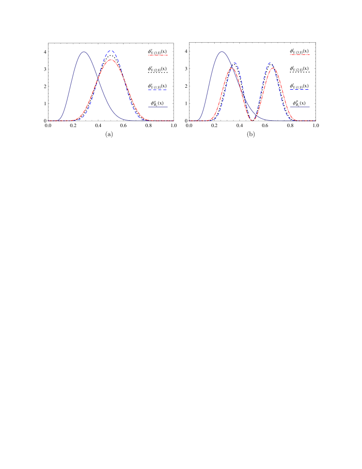
Figure 1: The distribution amplitudes of ${\phi}_{B_{c}}^{a,p}(x)$ and ${\phi}_{{\Upsilon}(nS)}^{v,t}(x)$.

II.5 Decay amplitudes

The Feynman diagrams for the ${\Upsilon}(nS)$ ${\to}$ $B_{c}{\pi}$ decay within the pQCD framework are shown in Fig.2, where (a) and (b) are factorizable topology; (c) and (d) are nonfactorizable topology.

Figure 2: Feynman diagrams for the ${\Upsilon}(nS)$ ${\to}$ $B_{c}{\pi}$ decay with the pQCD approach.

The decay amplitudes of ${\Upsilon}(nS)$ ${\to}$ $B_{c}P$ decay can be written as

$${\cal A}({\Upsilon}(nS){\to}B_{c}P)=\sqrt{2}G_{F}\frac{{\pi}C_{F}}{N}V_{cb}V_{uq}^{\ast}\,m_{\Upsilon}^{3}\,pf_{\Upsilon}f_{B_{c}}f_{P}\!\!\!\!\sum\limits_{i=a,b,c,d}\!\!\!\!{\cal A}_{\rm Fig.\ref{fig:amp}(i)},$$ (34)

where $C_{F}$ $=$ $4/3$ and the color number $N$ $=$ $3$.

The explicit expressions of ${\cal A}_{\rm Fig.\ref{fig:amp}(i)}$ are

$${\cal A}_{\rm Fig.\ref{fig:amp}(a)}\,=\,{\int}_{0}^{1}dx_{1}{\int}_{0}^{\infty}b_{1}db_{1}{\int}_{0}^{1}dx_{2}{\int}_{0}^{\infty}b_{2}db_{2}\,{\alpha}_{s}(t_{a})\,a_{1}(t_{a})\,E_{a}(t_{a})$$ (35)

$${\times}H_{a}(x_{1},x_{2},b_{1},b_{2})\,{\phi}_{\Upsilon}^{v}(x_{1})\,\Big{\{}{\phi}_{B_{c}}^{a}(x_{2})\,(x_{2}+r_{3}^{2}\,\bar{x}_{2})+{\phi}_{B_{c}}^{p}(x_{2})\,r_{2}\,r_{b}\Big{\}},$$

$${\cal A}_{\rm Fig.\ref{fig:amp}(b)}\,=\,{\int}_{0}^{1}dx_{1}{\int}_{0}^{\infty}b_{1}db_{1}{\int}_{0}^{1}dx_{2}{\int}_{0}^{\infty}b_{2}db_{2}\,{\alpha}_{s}(t_{b})\,a_{1}(t_{b})\,E_{b}(t_{b})$$ (36)

$${\times}H_{b}(x_{1},x_{2},b_{2},b_{1})\,\Big{\{}2\,r_{2}\,{\phi}_{B_{c}}^{p}(x_{2})\Big{[}r_{c}\,{\phi}_{\Upsilon}^{v}(x_{1})+x_{1}\,{\phi}_{\Upsilon}^{t}(x_{1})\Big{]}$$

$$-{\phi}_{B_{c}}^{a}(x_{2})\Big{[}{\phi}_{\Upsilon}^{v}(x_{1})\,(r_{2}^{2}\,x_{1}+r_{3}^{2}\,\bar{x}_{1})+{\phi}_{\Upsilon}^{t}(x_{1})\,r_{c}\Big{]}\Big{\}},$$

$${\cal A}_{\rm Fig.\ref{fig:amp}(c)}\,=\,{\int}_{0}^{1}dx_{1}{\int}_{0}^{\infty}db_{1}{\int}_{0}^{1}dx_{2}{\int}_{0}^{\infty}b_{2}db_{2}{\int}_{0}^{1}dx_{3}{\int}_{0}^{\infty}b_{3}db_{3}\,{\delta}(b_{1}-b_{2})\,{\alpha}_{s}(t_{c})$$ (37)

$${\times}\frac{C_{2}(t_{c})}{N}\,E_{c}(t_{c})\,H_{c}(x_{1},x_{2},x_{3},b_{2},b_{3})\,{\phi}_{P}^{a}(x_{3})\,\Big{\{}{\phi}_{B_{c}}^{p}(x_{2})\,{\phi}_{\Upsilon}^{t}(x_{1})\,r_{2}\,(x_{2}-x_{1})$$

$$\qquad+\ {\phi}_{B_{c}}^{a}(x_{2})\,{\phi}_{\Upsilon}^{v}(x_{1})\,\Big{[}(1+r_{2}^{2}-r_{3}^{2})\,(x_{1}-x_{3})+2\,r_{2}^{2}\,(x_{3}-x_{2})\Big{]}\Big{\}},$$

$${\cal A}_{\rm Fig.\ref{fig:amp}(d)}\,=\,{\int}_{0}^{1}dx_{1}{\int}_{0}^{\infty}db_{1}{\int}_{0}^{1}dx_{2}{\int}_{0}^{\infty}b_{2}db_{2}{\int}_{0}^{1}dx_{3}{\int}_{0}^{\infty}b_{3}db_{3}\,{\delta}(b_{1}-b_{2})\,{\alpha}_{s}(t_{d})$$ (38)

$${\times}\frac{C_{2}(t_{d})}{N}\,E_{d}(t_{d})\,H_{d}(x_{1},x_{2},x_{3},b_{2},b_{3})\,{\phi}_{P}^{a}(x_{3})\,\Big{\{}{\phi}_{B_{c}}^{p}(x_{2})\,{\phi}_{\Upsilon}^{t}(x_{1})\,r_{2}\,(x_{2}-x_{1})$$

$$\qquad+\ {\phi}_{B_{c}}^{a}(x_{2})\,{\phi}_{\Upsilon}^{v}(x_{1})\,(1-r_{2}^{2}-r_{3}^{2})\,(\bar{x}_{2}-x_{3})\Big{\}},$$

where ${\alpha}_{s}$ is the QCD coupling; $a_{1}$ $=$ $C_{1}$ $+$ $C_{2}/N$; $C_{1,2}$ is the Wilson coefficients; $r_{i}$ $=$ $m_{i}/m_{1}$. It can be easily seen that (1) the nonfactorizable contributions ${\cal A}_{\rm Fig.\ref{fig:amp}(c,d)}$ are color-suppressed with respect to the factorizable contributions ${\cal A}_{\rm Fig.\ref{fig:amp}(a,b)}$; (2) The twist-3 distribution amplitudes ${\phi}_{P}^{p,t}$ have no contribution to decay amplitudes.

The typical scales $t_{i}$ and the Sudakov factor $E_{i}$ are defined as

$$t_{a(b)}={\max}(\sqrt{-{\alpha}_{g}},\sqrt{-{\beta}_{a(b)}},1/b_{1},1/b_{2}),$$ (39)

$$t_{c(d)}={\max}(\sqrt{-{\alpha}_{g}},\sqrt{{|}{\beta}_{c(d)}{|}},1/b_{1},1/b_{2},1/b_{3}),$$ (40)

$$E_{a(b)}(t)={\exp}\{-S_{B_{c}}(t)\},$$ (41)

$$E_{c(d)}(t)={\exp}\{-S_{B_{c}}(t)-S_{P}(t)\},$$ (42)

$${\alpha}_{g}=\bar{x}_{1}^{2}m_{1}^{2}+\bar{x}_{2}^{2}m_{2}^{2}-\bar{x}_{1}\bar{x}_{2}t,$$ (43)

$${\beta}_{a}=m_{1}^{2}-m_{b}^{2}+\bar{x}_{2}^{2}m_{2}^{2}-\bar{x}_{2}t,$$ (44)

$${\beta}_{b}=m_{2}^{2}-m_{c}^{2}+\bar{x}_{1}^{2}m_{1}^{2}-\bar{x}_{1}t,$$ (45)

$${\beta}_{c}=x_{1}^{2}m_{1}^{2}+x_{2}^{2}m_{2}^{2}+x_{3}^{2}m_{3}^{2}-x_{1}x_{2}t-x_{1}x_{3}u+x_{2}x_{3}s,$$ (46)

$${\beta}_{d}=\bar{x}_{1}^{2}m_{1}^{2}+\bar{x}_{2}^{2}m_{2}^{2}+x_{3}^{2}m_{3}^{2}-\bar{x}_{1}\bar{x}_{2}t-\bar{x}_{1}x_{3}u+\bar{x}_{2}x_{3}s,$$ (47)

$$S_{B_{c}}(t)=s(x_{2},p_{2}^{+},1/b_{2})+2{\int}_{1/b_{2}}^{t}\frac{d{\mu}}{\mu}{\gamma}_{q},$$ (48)

$$S_{P}(t)=s(x_{3},p_{3}^{+},1/b_{3})+s(\bar{x}_{3},p_{3}^{+},1/b_{3})+2{\int}_{1/b_{3}}^{t}\frac{d{\mu}}{\mu}{\gamma}_{q},$$ (49)

where ${\alpha}_{g}$ and ${\beta}_{i}$ are the virtuality of the internal gluon and quark, respectively; ${\gamma}_{q}$ $=$ $-{\alpha}_{s}/{\pi}$ is the quark anomalous dimension; the expression of $s(x,Q,1/b)$ can be found in the appendix of Ref.pqcd1 .

The scattering functions $H_{i}$ in the subamplitudes ${\cal A}_{\rm Fig.\ref{fig:amp}(i)}$ are defined as

$$H_{a(b)}(x_{1},x_{2},b_{i},b_{j})\,=\,K_{0}(\sqrt{-{\alpha}_{g}}b_{i})\Big{\{}{\theta}(b_{i}-b_{j})K_{0}(\sqrt{-{\beta}}b_{i})I_{0}(\sqrt{-{\beta}}b_{j})+(b_{i}{\leftrightarrow}b_{j})\Big{\}},$$ (50)

$$H_{c(d)}(x_{1},x_{2},x_{3},b_{2},b_{3}) = \Big{\{}{\theta}(-{\beta})K_{0}(\sqrt{-{\beta}}b_{3})+\frac{{\pi}}{2}{\theta}({\beta})\Big{[}iJ_{0}(\sqrt{{\beta}}b_{3})-Y_{0}(\sqrt{{\beta}}b_{3})\Big{]}\Big{\}}$$ (51)

$${\times} \Big{\{}{\theta}(b_{2}-b_{3})K_{0}(\sqrt{-{\alpha}_{g}}b_{2})I_{0}(\sqrt{-{\alpha}_{g}}b_{3})+(b_{2}{\leftrightarrow}b_{3})\Big{\}},$$

where $J_{0}$ and $Y_{0}$ ($I_{0}$ and $K_{0}$) are the (modified) Bessel function of the first and second kind, respectively.

III Numerical results and discussion

In the rest frame of the ${\Upsilon}(nS)$ particle, branching ratio for the ${\Upsilon}(nS)$ ${\to}$ $B_{c}P$ weak decays can be written as

$${\cal B}r({\Upsilon}(nS){\to}B_{c}P)\ =\ \frac{1}{12{\pi}}\,\frac{p}{m_{{\Upsilon}}^{2}{\Gamma}_{{\Upsilon}}}\,{|}{\cal A}({\Upsilon}(nS){\to}B_{c}P){|}^{2}.$$ (52)

Table 2: Numerical values of the input parameters

Wolfenstein parameters pdg :	$A$ $=$ $0.814^{+0.023}_{-0.024}$, ${\lambda}$ $=$ $0.22537{\pm}0.00061$;
Masses of quarks pdg :	$m_{c}$ $=$ $1.67{\pm}0.07$ GeV,  $m_{b}$ $=$ $4.78{\pm}0.06$ GeV;
Gegenbauer moments:	$a_{2}^{\pi}$ (1 GeV) $=$ $0.17{\pm}0.08$ prd83 , $a_{4}^{\pi}$ (1 GeV) $=$ $0.06{\pm}0.10$ prd83 ,
	$a_{1}^{K}$ (1 GeV) $=$ $0.06{\pm}0.03$ jhep0605.004 , $a_{2}^{K}$ (1 GeV) $=$ $0.25{\pm}0.15$ jhep0605.004 ;
decay constant:	$f_{\pi}$ $=$ $130.41{\pm}0.20$ MeV pdg ,  $f_{K}$ $=$ $156.2{\pm}0.7$ MeV pdg ,
	$f_{B_{c}}$ $=$ $489{\pm}5$ MeV fbc ,  $f_{{\Upsilon}(1S)}$ $=$ $(676.4{\pm}10.7)$ MeV,
	$f_{{\Upsilon}(2S)}$ $=$ $(473.0{\pm}23.7)$ MeV,  $f_{{\Upsilon}(3S)}$ $=$ $(409.5{\pm}29.4)$ MeV.

The input parameters are collected in Table. 2. As for the decay constant $f_{{\Upsilon}}$, one can use the definition of decay constant,

$${\langle}0{|}\bar{b}{\gamma}^{\mu}{b}{|}{\Upsilon}{\rangle}=f_{{\Upsilon}}m_{{\Upsilon}}{\epsilon}_{{\Upsilon}}^{\mu}.$$ (53)

and relate $f_{{\Upsilon}}$ to the experimentally measurable leptonic branching ratio,

$${\Gamma}({\Upsilon}{\to}{\ell}^{+}{\ell}^{-})\,=\,\frac{4{\pi}}{27}{\alpha}_{\rm QED}^{2}\frac{f_{{\Upsilon}}^{2}}{m_{{\Upsilon}}}\sqrt{1-2\frac{m_{\ell}^{2}}{m_{{\Upsilon}}^{2}}}\Big{\{}1+2\frac{m_{\ell}^{2}}{m_{{\Upsilon}}^{2}}\Big{\}},$$ (54)

where ${\alpha}_{\rm QED}$ is the fine-structure constant, $m_{\ell}$ is the lepton mass and ${\ell}$ $=$ $e$, ${\mu}$, ${\tau}$.

The values of $f_{{\Upsilon}}$ determined from measurements are listed in Table.3. One may notice that there are some clear hierarchical relations among these decay constant. (1) The decay constants $f_{{\Upsilon}(nS)}^{e^{+}e^{-}}$ $<$ $f_{{\Upsilon}(nS)}^{{\mu}^{+}{\mu}^{-}}$ $<$ $f_{{\Upsilon}(nS)}^{{\tau}^{+}{\tau}^{-}}$ for the same radial quantum number $n$. There are two reasons. One is that the final phase space for decay into ${\ell}_{i}^{+}{\ell}_{i}^{-}$ states is more compact than that for ${\ell}_{j}^{+}{\ell}_{j}^{-}$ decay when the lepton family number $i$ $>$ $j$. The other is that branching ratio of ${\ell}_{i}^{+}{\ell}_{i}^{-}$ decay is relatively less than that of ${\ell}_{j}^{+}{\ell}_{j}^{-}$ decay with the lepton family number $i$ $<$ $j$. (2) There are also two reasons for the relation among the weighted average $f_{{\Upsilon}(1S)}$ $>$ $f_{{\Upsilon}(2S)}$ $>$ $f_{{\Upsilon}(3S)}$. One is that the possible phase space increases with the radial quantum number of upsilon due to $m_{{\Upsilon}(1S)}$ $<$ $m_{{\Upsilon}(2S)}$ $<$ $m_{{\Upsilon}(3S)}$. The other is that decay width of upsilon decreases with the radial quantum number $n$.

Table 3: Branching ratios for leptonic ${\Upsilon}(nS)$ decays and decay constants $f_{{\Upsilon}}$, where the last column is the weighted average, and errors come from mass, width and branching ratios.

decay mode	branching ratio	decay constant
${\Upsilon}(1S)$ ${\to}$ $e^{+}e^{-}$	$(2.38{\pm}0.11)\%$	$(664.2{\pm}23.1)$ MeV
${\Upsilon}(1S)$ ${\to}$ ${\mu}^{+}{\mu}^{-}$	$(2.48{\pm}0.05)\%$	$(677.9{\pm}14.7)$ MeV	$(676.4{\pm}10.7)$ MeV
${\Upsilon}(1S)$ ${\to}$ ${\tau}^{+}{\tau}^{-}$	$(2.60{\pm}0.10)\%$	$(683.3{\pm}21.1)$ MeV
${\Upsilon}(2S)$ ${\to}$ $e^{+}e^{-}$	$(1.91{\pm}0.16)\%$	$(471.0{\pm}39.1)$ MeV
${\Upsilon}(2S)$ ${\to}$ ${\mu}^{+}{\mu}^{-}$	$(1.93{\pm}0.17)\%$	$(473.5{\pm}40.3)$ MeV	$(473.0{\pm}23.7)$ MeV
${\Upsilon}(2S)$ ${\to}$ ${\tau}^{+}{\tau}^{-}$	$(2.00{\pm}0.21)\%$	$(475.2{\pm}44.5)$ MeV
${\Upsilon}(3S)$ ${\to}$ ${\mu}^{+}{\mu}^{-}$	$(2.18{\pm}0.21)\%$	$(407.6{\pm}38.2)$ MeV	$(409.5{\pm}29.4)$ MeV
${\Upsilon}(3S)$ ${\to}$ ${\tau}^{+}{\tau}^{-}$	$(2.29{\pm}0.30)\%$	$(412.2{\pm}45.9)$ MeV

Table 4: Branching ratios for the ${\Upsilon}(nS)$ ${\to}$ $B_{c}{\pi}$, $B_{c}K$ decays, where previous results are calculated with the coefficient $a_{1}$ $=$ $1.05$.

	Ref. ijma14	Ref. adv2013	Ref. 691261	this work
$10^{11}{\times}{\cal B}r({\Upsilon}(1S){\to}B_{c}{\pi})$	6.91	2.8	5.03	$7.40^{+0.51+0.90+0.88+0.30}_{-0.49-0.57-1.01-0.28}$
$10^{11}{\times}{\cal B}r({\Upsilon}(2S){\to}B_{c}{\pi})$	…	…	…	$6.29^{+0.43+0.70+0.55+1.67}_{-0.41-0.45-0.62-0.44}$
$10^{11}{\times}{\cal B}r({\Upsilon}(3S){\to}B_{c}{\pi})$	…	…	…	$6.57^{+0.45+0.69+0.44+1.55}_{-0.43-0.45-0.51-0.86}$
$10^{12}{\times}{\cal B}r({\Upsilon}(1S){\to}B_{c}K)$	5.03	2.3	3.73	$5.67^{+0.42+0.71+0.68+0.24}_{-0.40-0.45-0.77-0.23}$
$10^{12}{\times}{\cal B}r({\Upsilon}(2S){\to}B_{c}K)$	…	…	…	$4.85^{+0.36+0.55+0.45+1.27}_{-0.34-0.35-0.42-0.36}$
$10^{12}{\times}{\cal B}r({\Upsilon}(3S){\to}B_{c}K)$	…	…	…	$5.09^{+0.38+0.55+0.35+1.15}_{-0.36-0.35-0.34-0.71}$

Our numerical results on the $CP$-averaged branching ratios for the ${\Upsilon}(nS)$ ${\to}$ $B_{c}{\pi}$, $B_{c}K$ decays are displayed in Table 4, where the uncertainties come from the CKM parameters, the renormalization scale ${\mu}$ $=$ $(1{\pm}0.1)t_{i}$, masses of $b$ and $c$ quarks, hadronic parameters including decay constants and Gegenbauer moments, respectively. The following are some comments.

(1) Branching ratios for the bottom-changing ${\Upsilon}(nS)$ ${\to}$ $B_{c}{\pi}$, $B_{c}K$ weak decays with the pQCD approach have the same magnitude of order as previous estimation in Refs. ijma14 ; adv2013 ; 691261 . Compared with the NF and QCDF approaches, there are more contributions from the nonfactorizable decay amplitudes ${\cal A}_{\rm Fig.\ref{fig:amp}(c,d)}$ with the pQCD approach, which may be the reason of why the pQCD’s results are slightly larger than previous ones.

(2) Because of hierarchical relation between the CKM factors ${|}V_{cb}V_{us}^{\ast}{|}$ $>$ ${|}V_{cb}V_{ud}^{\ast}{|}$, in general, there is relation between branching ratios ${\cal B}r({\Upsilon}(nS){\to}B_{c}{\pi})$ $>$ ${\cal B}r({\Upsilon}(nS){\to}B_{c}K)$.

(3) Because the relations among masses $m_{{\Upsilon}(3S)}$ $>$ $m_{{\Upsilon}(2S)}$ $>$ $m_{{\Upsilon}(1S)}$ resulting in that the momentum and phase space of final states increase with the radial quantum number $n$, in addition, the relation among decay widths ${\Gamma}_{{\Upsilon}(3S)}$ $<$ ${\Gamma}_{{\Upsilon}(2S)}$ $<$ ${\Gamma}_{{\Upsilon}(1S)}$ (see Table. 1), in principle, it is expected that there should be relations among branching ratios ${\cal B}r({\Upsilon}(3S){\to}B_{c}P)$ $>$ ${\cal B}r({\Upsilon}(2S){\to}B_{c}P)$ $>$ ${\cal B}r({\Upsilon}(1S){\to}B_{c}P)$ for the same pseudoscalar meson $P$. But the results in Table. 4 is not the way one expected it to be. Why? The reason is that the decay amplitudes with the pQCD approach is proportional to decay constant $f_{{\Upsilon}(nS)}$, and the fact of that the difference among final phase spaces is small, hence there is an approximation,

$${\cal B}r({\Upsilon}(1S){\to}B_{c}P):{\cal B}r({\Upsilon}(2S){\to}B_{c}P):{\cal B}r({\Upsilon}(3S){\to}B_{c}P)$$ (55)

$${\propto} \frac{f_{{\Upsilon}(1S)}^{2}}{{\Gamma}_{{\Upsilon}(1S)}}:\frac{f_{{\Upsilon}(2S)}^{2}}{{\Gamma}_{{\Upsilon}(2S)}}:\frac{f_{{\Upsilon}(3S)}^{2}}{{\Gamma}_{{\Upsilon}(3S)}}\ {\simeq}\ 1.2:1:1.2.$$

(3) Branching ratio for the ${\Upsilon}(nS)$ ${\to}$ $B_{c}{\pi}$ decay is a few times of $10^{-11}$. So the nonleptonic ${\Upsilon}(nS)$ ${\to}$ $B_{c}{\pi}$ weak decays could be sought for with some priority at the running LHC and the forthcoming SuperKEKB. For example, the production cross section of ${\Upsilon}(nS)$ in p-Pb collision can reach up to a few ${\mu}b$ with the LHCb jhep1407 and ALICE plb740 detectors at LHC. Over $10^{11}$ ${\Upsilon}(nS)$ particles per 100 $fb^{-1}$ data collected at LHCb and ALICE are in principle available, which corresponds to a few tens of ${\Upsilon}(nS)$ ${\to}$ $B_{c}{\pi}$ events.

(4) There are many uncertainties on our results. The CKM factors can bring about 7% uncertainty on the prediction of branching ratio. More than 10% uncertainty come from the variation of typical scale $t_{i}$. The effects of masses of $m_{b}$ and $m_{c}$ on branching ratio decrease with the radial quantum number $n$. Compared with the ${\Upsilon}(1S)$ weak decays, hadronic parameters give a noticeable uncertainty on ${\Upsilon}(2S,3S)$ weak decays due to large errors on the decay constants $f_{{\Upsilon}(2S,3S)}$ relative to $f_{{\Upsilon}(1S)}$. Other factors, such as the contributions of higher order corrections to HME, relativistic effects and so on, which are not considered here, deserve the dedicated study. Our results just provide an order of magnitude estimation.

IV Summary

The ${\Upsilon}(nS)$ weak decay is allowable within the standard model, although branching ratio is tiny compared with the strong and electromagnetic decays. It is expected that the ${\Upsilon}(nS)$ particles could be produced and collected copiously at the high-luminosity dedicated heavy-flavor factories. It seems to have a good opportunity and a realistic possibility to search for the ${\Upsilon}(nS)$ weak decay experimentally. In this paper, we study the color-favored bottom-changing ${\Upsilon}(nS)$ ${\to}$ $B_{c}{\pi}$, $B_{c}K$ weak decays with the pQCD approach just to offer a ready reference to experimental analysis. It is found that branching ratios for the ${\Upsilon}(nS)$ ${\to}$ $B_{c}{\pi}$ decays are the order of ${\cal O}(10^{-11})$, which might be detectable in future experiments.

References

• (1) S. Herb et al., Phys. Rev. Lett. 39, 252 (1977).
• (2) W. Innes et al., Phys. Rev. Lett. 39, 1240 (1977).
• (3) K. Olive et al. (Particle Data Group), Chin. Phys. C 38, 090001 (2014).
• (4) P. Franzini, J. Lee-Franzini, Ann. Rev. Nucl. Part. Sci. 33, 1 (1983).
• (5) S. Okubo, Phys. Lett. 5, 165 (1963).
• (6) G. Zweig, CERN-TH-401, 402, 412 (1964).
• (7) J. Iizuka, Prog. Theor. Phys. Suppl. 37-38, 21 (1966).
• (8) C. Patrignani, T. Pedlar, J. Rosner, Annu. Rev. Nucl. Part. Sci. 63, 21 (2013).
• (9) H. Li, Phys. Rev. D 52, 3958 (1995).
• (10) C. Chang, H. Li, Phys. Rev. D 55, 5577 (1997).
• (11) T. Yeh, H. Li, Phys. Rev. D 56, 1615 (1997).
• (12) Ed. A. Bevan et al., Eur. Phys. J. C 74, 3026, (2014).
• (13) T. Gershon, M. Needham, C. R. Physique 16, 435 (2015).
• (14) M. Sanchis-Lozano, Z. Phys. C 62, 271 (1994).
• (15) K. Sharma, R. Verma, Int. J. Mod. Phys. A 14, 937 (1999).
• (16) R. Dhir, R. Verma, A. Sharma, Adv. in High Energy Phys. 2013, 706543 (2013).
• (17) M. Beneke et al., Phys. Rev. Lett. 83, 1914 (1999).
• (18) M. Beneke et al., Nucl. Phys. B 591, 313 (2000).
• (19) M. Beneke et al., Nucl. Phys. B 606, 245 (2001).
• (20) C. Bauer et al., Phys. Rev. D 63, 114020 (2001).
• (21) C. Bauer, D. Pirjol, I. Stewart, Phys. Rev. D 65, 054022 (2002).
• (22) C. Bauer et al., Phys. Rev. D 66, 014017 (2002).
• (23) M. Beneke et al., Nucl. Phys. B 643, 431 (2002).
• (24) G. Buchalla, A. Buras, M. Lautenbacher, Rev. Mod. Phys. 68, 1125, (1996).
• (25) G. Legage, S. Brodsky, Phys. Rev. D 22, 2157 (1980).
• (26) T. Kurimoto, H. Li, A. Sanda, Phys. Rev. D 65, 014007 (2001).
• (27) P. Ball, V. Braun, Y. Koike, K. Tanaka, Nucl. Phys. B 529, 323 (1998).
• (28) P. Ball, V. Braun, A. Lenz, JHEP, 0605, 004, (2006).
• (29) G. Legage et al., Phys. Rev. D 46, 4052 (1992).
• (30) G. Bodwin, E. Braaten, G. Legage, Phys. Rev. D 51, 1125 (1995).
• (31) N. Brambilla et al., Rev. Mod. Phys. 77, 1423 (2005).
• (32) B. Xiao, X. Qin, B. Ma, Eur. Phys. J. A 15, 523 (2002).
• (33) A. Khodjamirian, Th. Mannel, N. Offen, Y. Wang, Phys. Rev. D 83, 094031 (2011).
• (34) T. Chiu, T. Hsieh, C. Huang, K. Ogawa, Phys. Lett. B 651, 171 (2007).
• (35) J. Sun et al., Adv. in High Energy Phys. 2015, 691261 (2015).
• (36) R. Aaij et al. (LHCb Collaboration), JHEP 1407, 094 (2014).
• (37) B. Abelev et al. (ALICE Collaboration), Phys. Lett. B 740, 105 (2015).