Optimizing Timing of High-Success-Probability Quantum Repeaters

Abstract

Optimizing a connection through a quantum repeater network requires careful attention to the photon propagation direction of the individual links, the arrangement of those links into a path, the error management mechanism chosen, and the application’s pattern of consuming the Bell pairs generated. We analyze combinations of these parameters, concentrating on one-way error correction schemes (1-EPP) and high success probability links (those averaging enough entanglement successes per round trip time interval to satisfy the error correction system). We divide the buffering time (defined as minimizing the time during which qubits are stored without being usable) into the link-level and path-level waits. With three basic link timing patterns, a path timing pattern with zero unnecessary path buffering exists for all $3^{h}$ combinations of $h$ hops, for Bell inequality violation experiments (B class) and Clifford group (C class) computations, but not for full teleportation (T class) computations. On most paths, T class computations have a range of Pareto optimal timing patterns with a non-zero amount of path buffering. They can have optimal zero path buffering only on a chain of links where the photonic quantum states propagate counter to the direction of teleportation. Such a path reduces the time that a quantum state must be stored by a factor of two compared to Pareto optimal timing on some other possible paths.

I Introduction

Distributed, entangled quantum states are useful for a variety of purposes, including creation of provably secure, classical random bits to be used as keys for encryption ekert1991qcb ; distributed physical reference frames for clock synchronization and optical long-baseline interferometry for astronomy PhysRevLett.87.129802 ; chuang2000qclk ; PhysRevLett.109.070503 ; and distributed quantum computation crepeau:_secur_multi_party_qc ; broadbent2009universal ; Tani:2012:EQA:2141938.2141939 .

In the early days of quantum information research, Bennett et al. recognized that the component qubits of an entangled state may be held at different times in different locations, which they called time-separated Bell pairs PhysRevA.54.3824 . We can apply this principle to group applications into three categories, depending on their timing patterns: Bell inequality violations and QKD (B class), which allow post-selection of successful trials; Clifford group computations, such as creating cluster states (C class), which allow post-operation application of Pauli frame corrections; and full teleportation and non-Clifford computations (T class), which require completion of all Pauli corrections before proceeding. Each class places different demands on the timing of operations at each node, and ultimately affects the efficiency of a repeater network. These three patterns are summarized in Tab. 1.

Class	Name	reception success notification	Pauli frame propagation
B	Bell (Bell inequality violations, QKD)	I	I
C	Clifford group computation	W	I
T	General (non-Clifford group) computation, teleportation	W	W

Table 1: Application usage patterns. The label ’W’ indicates that the class must wait for the condition to be fulfilled before proceeding to the next step using the quantum memory, while ’I’ indicates that the application may proceed immediately, without waiting.

Creating distributed quantum states over a distance is the work of a chain of quantum repeaters dur:PhysRevA.59.169 . A quantum repeater has three functions: creating base-level entanglement (typically a Bell pair) across a distance; coupling two entangled states to lengthen entanglement; and managing errors. Repeater chains may use purification as an error detection mechanism dur:PhysRevA.59.169 , or quantum error correction (QEC) knill96:concat-arxiv ; PhysRevA.79.032325 ; PhysRevLett.104.180503 ; muralidharan15:_ultrafast-generations . In this paper we focus on QEC-based repeaters, which allow one-way classical communication to be effective. Links and nodes will be organized into large-scale networks, which in turn may connect into a quantum Internet kimble08:_quant_internet ; van-meter14:_quantum_networking ; PhysRevA.93.042338 . A chain of repeaters selected from among the network’s links for the purposes of communicating between two given nodes is a path.

The performance of a path of quantum repeaters, in terms of end-to-end Bell pair generation rate and fidelity, is largely determined by the efficient use of buffer memory in the repeater nodes . Efficiency in turn is driven by the success probability per entanglement trial (determined by link hardware and channel loss), trial repetition rate (determined by link architecture and channel length), timing of the use of path elements (the focus of this article), and the timing of consumption of the end-to-end Bell pairs (determined by the application communication pattern, above).

The arrangement of components in a repeater link dictates the propagation direction and travel distance of photons in the channel. Some link timing patterns have a polarity, or direction of propagation, while others are symmetric, with two photons originating in the middle or meeting in the middle.

A path can be composed of links oriented in a large number of possible patterns: $2^{h}$ for $h$ hops, or $3^{h}$ if we allow interspersed unpolarized links. If the probability of photon reception is low, operation will be highly asynchronous, but when the probability is high, we can coordinate the relative timing of operations on each link. In this article, we present our analysis of several classes of path timing patterns, focusing on paths with polarity to analyze systems with the goal of minimizing memory buffering time and maximizing performance.

We find that B and C class applications can always achieve the minimum buffer timing of a single end-to-end round trip (or slightly less for B class on many paths), including the time awaiting confirmation of entanglement across each link. For T class applications, an optimal timing pattern exists only for a path composed of links with photons propagating counter to the direction of teleportation. In general, the minimum amount of time that the qubits building a distributed quantum state dwell in memory, including awaiting the link level acknowledgement, varies by up to a factor of two, depending on path link pattern, error management mechanism, and application pattern.

These results advance our understanding of how to engineer quantum repeater networks for deployment in the real world, by establishing the “best best-case scenario” and the “worst best-case scenario” for performance.

II Elementary Timing Patterns

Before discussing the composition of link timing choices to create path timing sequences, we must discuss in more detail the individual link level timing patterns, the relationship to error management (purification or correction), and the relationship to how the application uses entanglement.

In all of the examples in this article, we will assume “forward” teleportation, drawn left to right in the diagrams. Bell inequality violation experiments and QKD do not have such end-to-end application-level polarity. In some cases, this allows them to behave apparently atemporally, with qubits measured and released at the right end of a connection before photons are created at the left end. The resulting classical data is not useful until Pauli frame corrections are received bertlmann12 , but our focus in this article is the consumption of quantum resources (especially memory time).

II.1 Link Level Timing

There are three major link architectures classified by their timing pattern, $M\rightarrow M$ (and $M\leftarrow M$), $M\rightarrow I\leftarrow M$, and $M\leftarrow S\rightarrow M$, summarized in Tab. 2 and illustrated in Fig. 1 van-meter14:_quantum_networking . We will use $t$ for one-way link propagation times, and $T_{E}$ for one-way propagation end-to-end along an entire path. When necessary to discuss the latency of a single link within a path, we will refer to $t_{j}$ for the $i$th link.

$M\rightarrow M$ ($M\leftarrow M$) can be considered to be a sender-receiver (receiver-sender) arrangement. A link may be composed of an emitter at the transmitting end, and another emitter coupled with an interference apparatus at the receiving end such that the combination behaves as a receiver hong-PhysRevLett.59.2044 ; PhysRevA.59.1025 ; duan2001ldq ; duan:RevModPhys.82.1209 . Other physical mechanisms, such as qubus links, also exhibit the $M\rightarrow M$ pattern spiller05:_qubus .

$M\rightarrow I\leftarrow M$ uses two transmitters and a Bell state analyzer (BSA, e.g., Hong-Ou-Mandel dip) positioned halfway in between the two to erase which-path information, leaving the two stationary qubits in an entangled state hong-PhysRevLett.59.2044 ; PhysRevA.59.1025 ; duan:RevModPhys.82.1209 . This approach has seen substantial experimental success hucul2014modular ; sipahigil:PhysRevLett.108.143601 ; bernien2013heralded .

$M\leftarrow S\rightarrow M$ uses an entangled photon pair source (EPPS) at the midpoint of the link, sending one photon toward each of two receivers jones2015design . Satellite-based repeater links are also $M\leftarrow S\rightarrow M$, although the buffering latency is determined by the terrestrial classical communication time rather than the actual propagation time from the satellite aspelmeyer2003ldq ; PhysRevA.91.052325 ; PhysRevLett.94.150501 .

Success probability per trial remains a critical Achilles heel in experimental work, with values around $10^{-5}$ hucul2014modular . The no-cloning theorem wootters:no-cloning ; PhysRevLett.78.3217 dictates that attempts to directly transmit quantum states encoded in an error correcting code require that more than fifty percent of the qubits arrive, $P_{r}>0.5$, where $P_{r}$ is the probability of successful reception of the photon. Because technology sufficient to achieve this level of success remains far off, we must instead first create entangled Bell pairs, before attempting to use them for communication. We refer to a link architecture that confirms the creation of Bell pairs as acknowledged entanglement creation, and the supporting classical messaging protocol as AEC van-meter07:banded-repeater-ton ; aparicio11:repeater-proto-design . We make the distinction from link-level heralding, as heralding is a local event confirming successful entanglement, where that information may be used locally or transmitted to the partner.

We must buffer the qubits at each end until the necessary classical messages can arrive. All three link architectures require decoherence lifetime sufficient for retaining high fidelity after a full round trip time ($2t$), but the location of that memory buffering and the reason for it varies. During the time period in which the memory qubit is entangled with an in-flight photonic state, or we are awaiting acknowledgement of entanglement success or failure, we refer to the memory as being in the half-entangled state aparicio11:repeater-proto-design . Tab. 2 lists the half-entangled quantum time (Q) during which a stationary qubit is entangled with an in-flight photon and the half-entangled classical time (C) during which the photon has arrived or failed to arrive, but we are awaiting confirmation. These times are marked in Fig. 1. In $M\rightarrow M$, all of the time is at the transmitting end, whereas in $M\rightarrow I\leftarrow M$ and $M\leftarrow S\rightarrow M$ the buffering time is evenly split between the two ends. Assuming the decoherence process is memoryless and the memory types at both ends are identical, the net decoherence on the resulting Bell pair caused by storing a single memory for time $2t$ is the same as for storing two memories for time $t$ each.

The figure shows a single qubit at each node, but we can enhance performance by using more qubits at each end. The analysis here assumes that the two arms of $M\rightarrow I\leftarrow M$ and $M\leftarrow S\rightarrow M$ links are balanced in both latency and memory capacity, but that need not be so.

Link	long name	“left” end			“right” end
		Tx/Rx	Q	C	Tx/Rx	Q	C	L:R buffer balance	rep rate
$M\rightarrow M$	SenderReceiver	Tx	$t$	$t$	Rx	0	0	$P_{r}^{-1}:1$	1/RTT
$M\leftarrow M$	ReceiverSender	Rx	0	0	Tx	$t$	$t$	1:$P_{r}^{-1}$	1/RTT
$M\rightarrow I\leftarrow M$	MeetInTheMiddle	Tx	$t/2$	$t/2$	Tx	$t/2$	$t/2$	1:1	2/RTT
$M\leftarrow S\rightarrow M$	MidpointSource	Rx	$0$	$t$	Rx	$0$	$t$	1:1	many/RTT

Table 2: Link architectures. Each end (conventionally “left” and “right”) is identified as transmitter (Tx) or receiver (Rx). Q and C are quantum and classical signal propagation wait times, the half-entangled time in which a buffer memory is awaiting confirmation of entanglement success with a partner. rep rate is the rate at which a given buffer qubit can be used in an entanglement attempt. RTT is the link signal round trip time, $2t$.

Regime	Reception Probability Range	D/G	Description	Suitable timing architecture
low probability	$P_{r}\lessapprox\frac{2n}{N_{T}}$	G	Prob. too low for coordinated operation	Fully async, ACKed 1-EPP or 2-EPP building E2E Bell pairs
high probability	$\frac{2n}{N_{T}}\lessapprox P_{r}<0.5$	G	Using many transmitters, high prob. of enough qubits being received to compose full QEC block size, but not above no-cloning loss limit	ACKed, optimized 1-EPP building E2E Bell pairs
high prob. (extended)	$0.5<P_{r}<\alpha$	G	Above no-cloning loss limit, but not yet practically so	ACKed, optimized 1-EPP building E2E Bell pairs
very high probability	$\alpha<P_{r}<1.0-\epsilon$	D	Above no-cloning loss limit; more than half the qubits will arrive, allowing QEC reconstruction of state	fully 1-EPP, direct transmission of state in QEC block
perfect	$1.0-\epsilon\leq P_{r}$	D	Error management does not need to account for loss	direct transmission (gate error rates permitting)

Table 3: Matching probability regimes with appropriate entanglement purification patterns. $P_{r}$ is the photon reception or entanglement creation probability. $N_{T}$ is the number of transmitter qubits in an $M\rightarrow M$ link, and $n$ is the block size in an [[$n$,$k$,$d$]] quantum error correction code. $\alpha$ is chosen to assure low probability of $<\frac{\lfloor(n+1)/2\rfloor}{n}$ successes in every block operation across the entire path (see Sec. IV.2). In the “D/G” column, “D” denotes direction transmission of valuable quantum data, while “G” denotes creation of generic quantum states (e.g., Bell pairs) which later are used to teleport quantum data. In this paper, we focus on the high probability and high probability (extended) regimes.

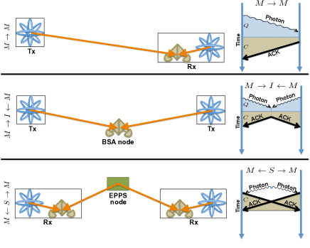
Figure 1: Hardware arrangements for $M\rightarrow M$, $M\rightarrow I\leftarrow M$, and $M\leftarrow S\rightarrow M$ links. Stationary memories are represented by the atom symbols. For the $M\rightarrow M$ link, the transmitting (left) end of the link should have more memories than the receiving (right) end, in proportion to the entanglement success probability. Timing patterns and memory buffering times are shown in the diagrams on the right. The $M\rightarrow M$ link has transmitter-receiver polarity, evidenced by the trapezoid shape. Shaded areas marked $Q$ indicate delay during quantum signal propagation, while shaded areas marked $C$ await classical signal propagation.

II.2 Error Management Timing

In 1996, Bennett et al. bennett1996pne ; PhysRevA.54.3824 , Knill and Laflamme knill96:concat-arxiv , and Deutsch et al. PhysRevLett.77.2818 introduced means of managing errors in distributed Bell states. An entanglement purification protocol (EPP) takes several distributed, mixed quantum states and reduces them to a smaller number of higher-fidelity states. Some of the states are assigned to be sacrificial test tools, and others are assigned to be the output states. Essentially, an EPP begins with a proposition, such as, “This Bell pair is in the state $\left|\Psi^{+}\right\rangle$,” and uses the test tools to test the correctness of that proposition.

Among the several mechanisms, the primary distinction is whether communication is one way (1-EPP) or two way (2-EPP). A 2-EPP has three significant advantages: it is robust against loss of qubits, its resource requirements are low, and the procedures are simple. A 1-EPP also has advantages: it can use any known quantum error correcting code, it integrates well with notions of error-corrected distributed computation, and most importantly, reduces the need to buffer states while waiting for classical communication, allowing a quantum network to propagate signals end to end in a hop-by-hop fashion similar to classical networks.

The simplest 2-EPP is a $2\rightarrow 1$ protocol, in which one Bell pair is used to test the parity of a second. A cnot gate is performed between the qubits of the two Bell pairs at each node, the target qubit is measured, and the results are exchanged. If the measurement results agree, confidence that the initial proposition about the state is correct is strengthened. If the results disagree, even the remaining Bell pair must be discarded.

1-EPP mechanisms can either retain the received state in an error corrected form, or reduce the initial set of Bell pairs to unencoded Bell pairs, much like the simplest 2-EPP. It is known that 1-EPP is not robust against loss of more than 50% of the Bell pairs.

Our natural preference is for the 1-EPP, due to its low buffering requirements. However, the number of qubits per node and the required number of Bell pair creation successes in a single burst of trials is high (see Sec. IV). For a surface code of distance $d$, we need $d$ successes in the burst to achieve the optimal timing addressed here. For a CSS code of $[[n,k,d]]$, we need a burst of $n$ entanglement successes.

II.3 Application Timing and Buffer Time

Fig. 2 illustrates the timing and actions of the three application categories listed in Tab. 1.

Our waiting time can be divided into two categories: the link wait time $T^{H}$ and the path wait time $T^{P}$. The link wait time $T^{H}$ is spent waiting for the classical entanglement success/failure acknowledgment to arrive, also known as the half-entangled time. For the C and T classes, which expect to execute additional quantum operations on qubits at each end, we cannot use a qubit that is entangled with a lost photon, as the photon loss leaves us in a completely mixed state. B class applications, in contrast, only measure the qubit, and can post-select for entanglement success. When we have multiple qubits in flight, this acknowledgment signal serves as a selection signal, telling us which qubit (if any) to use, as in the figure. Over a single $M\rightarrow M$ hop, the half-entangled wait times for the separate classes are

$$T^{H}_{B} =0$$

$$T^{H}_{C} =T^{H}_{T}=2t.$$ (1)

During the path wait time, $T^{P}$, we cannot perform certain quantum operations as we are awaiting either Pauli frame correction information or the qubit-to-qubit matching information for entanglement swapping (Sec. III.1). B class operations can apply Pauli frame corrections to the classical measurement results long afterwards, as with the photon reception post-selection. C class operations may proceed with Clifford group and measurement quantum operations as soon as photon reception is confirmed, with Pauli frame correction to follow later. T class operations, which required non-Clifford group operations, cannot proceed at the destination until the Pauli frame correction is received and applied, giving

$$T^{P}_{B} =T^{P}_{C}=0$$

$$T^{P}_{T} =t.$$ (2)

In general, $T^{H}_{C}=T^{H}_{T}$ and $T^{P}_{C}=T^{P}_{B}$. We define total buffer times for B, C, and T classes to be $T_{B}$, $T_{C}$, and $T_{T}$, respectively,

$$T_{B} =T^{H}_{B}+T^{P}_{B}=0$$

$$T_{C} =T^{H}_{C}+T^{P}_{C}=2t$$

$$T_{T} =T^{H}_{T}+T^{P}_{T}=3t,$$ (3)

representing the cumulative decoherence suffered by our quantum data.

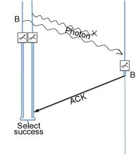
(a) B class

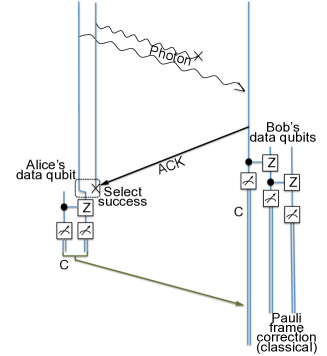
(b) C class

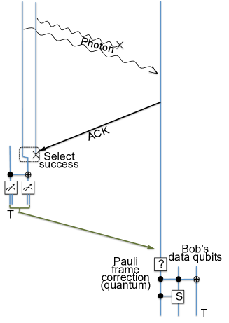
(c) T class

Figure 2: Timing for application classes over a single forward-propagating link.

III Path Timing Patterns

Our goal is to determine the minimum achievable memory buffering time, taking into account the application pattern and various link arrangements.

III.1 Building Long-Distance Entanglement

The original proposal for quantum repeaters used entanglement swapping: Bob holds a Bell pair with Alice, and a second Bell pair with Charlie, and performs a Bell state measurement using the two qubits PhysRevLett.71.4287 ; briegel98:_quant_repeater . This disentangles Bob’s two qubits and splices the original shorter Bell pairs into one longer one. However, in order to complete the operation, a Pauli frame correction must be applied at one end, and both ends must be informed of the completion of the operation. The propagation of these messages is one of the key constraints on system performance.

The original proposal used entanglement swapping at the physical level. Jiang et al. proposed using it at the logical level PhysRevA.79.032325 . Fowler et al. used the surface code-specific approach of coupling together small segments of the surface code to form a single, long, narrow surface PhysRevLett.104.180503 .

III.2 Path Basics

A path is a concatenated sequence of links through a network chosen to connect a source and destination van-meter:qDijkstra . The end-to-end latency of the path is just the sum of the individual link latencies,

$$T_{E}=\sum_{j}t_{j}.$$ (4)

This value has some relationship to the path performance and to the decoherence suffered by stationary memories. Exploring that relationship, which is not straightforward, is the goal of this paper.

If memory decoherence is a memoryless process, the sum of the buffer times all along the path determines total decoherence.

In planning to eliminate unnecessary buffering, we care about two factors:

1. the total amount of unnecessary buffering, which determines the unnecessary decoherence suffered; and

2. the spatial distribution of the unnecessary buffering, which determines the impact on aggregate network performance.

To minimize buffer wait times, we coordinate action across the entire path using one or more trigger signals. The trigger may propagate left to right (forward) or right to left (reverse). We may also trigger from the middle of the path (inside out), or simultaneously from both ends toward the middle (outside in). Each link may transmit photons in the same direction as the trigger (co-propagating) or in the opposite direction (counter-propagating). The design decision of the trigger and link propagation pattern has a significant effect on buffer memory times.

Entanglement swapping information becomes available after the neighboring link has confirmation of photon reception, either at the sending or receiving end. In Figs. 3 and 4, the path wait times $T^{P}$ (whether we are waiting for Pauli frame information or entanglement swapping information) are illustrated with red arrows outside of the trapezoids representing link timing. The link wait times $T^{H}$ are not directly represented in the figures, but are understood to be along the long edge of each trapezoid.

III.3 Forward Propagation, Flat Timing

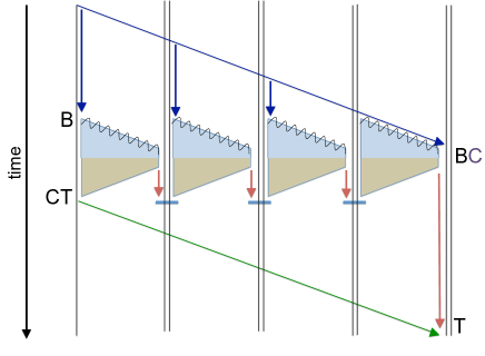
(a) Forward propagation links, flat timing

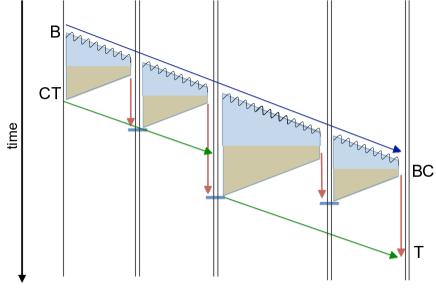
(b) Forward triggered with varied-length hops, not Pareto optimal

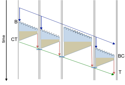
(c) Varied-length hops with corrected trigger

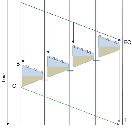
(d) Bell matched timing

Figure 3: Timing for forward operation with acknowledged link-level entanglement on a forward-propagating path. Blue arrows are the timing trigger. Green arrows are propagation of Bell state measurement results used as Pauli frame corrections. Red arrows indicate memory hold time waiting for BSA or final Pauli frame correction. (a) Flat-timed 1-EPP repeaters. The red arrows here sum to one end-to-end round-trip time for the C and T classes. (b) Forward propagation with uneven link latencies and a simple trigger, causing the “long pole” to extend below the green arrow, violating the first Pareto optimality condition. (c) The same path with corrected trigger, giving Pareto optimal timing. (d) The Bell matched timing, optimal for all three classes.

After selecting an error management mechanism, we can compose links into a path, then add a path trigger pattern and application Bell pair consumption information to project behavior. This can be illustrated graphically, and we can read the required buffer timings directly off of each diagram, as in Figs. 3 and 4.

As an example, consider the basic operation of 1-EPP repeaters, as described by Jiang et al. and Fowler et al. The analysis in both papers originally assumed synchronous operation across all links, as illustrated in Fig. 3a. While this is not strictly necessary, it simplifies the exposition and basic performance analysis. The exact timing of the BSA at each node can in fact be independent, as long as the BSA operations along the chain can be mapped to the correct end-to-end session.

However, in the figure, the red arrows indicate time where only one side of a planned entanglement swap is ready. For this path, all three application classes have unnecessary path buffering at every node except the end points. For the B and C application classes, this is the only unnecessary buffering incurred, giving us

$$T^{P}_{B}=T^{P}_{C}=\sum_{j=2}^{h}t_{j}=T_{E}-t_{1}$$ (5)

noting that the first hop is left out. The T application class requires us to wait at the right end until the Pauli frame information arrives from the left end, giving

$$T^{P}_{T} =\sum_{j=2}^{h}t_{j}+t_{h}+T_{E}$$

$$=2T_{E},\text{when all links have the same $t_{j}$.}$$ (6)

or one end-to-end round-trip time. B and C class buffering is evenly spread along the path except for the last node. The additional buffering time for the T class is entirely at the right end.

III.4 Forward Propagation, Other Timing Patterns

The flat timing pattern is only one possible pattern for this fixed arrangement of hops. Different timing patterns are achieved by sliding the link timing trapezoids up and down by adjusting the trigger pattern. Some moves result in a global reduction the buffering time, others a global increase. Some moves do not change the global sum, but alter the location of the buffering.

Fig. 3b shows an obvious but poor choice of timing pattern, using a single forward trigger and immediately firing each link on the trigger. This pattern is worse than flat timing, with twice the buffering for B and C classes and the same or worse buffering for T class,

$$T^{P}_{B}=T^{P}_{C} =\sum_{j=2}^{h}2t_{j}$$ (7)

$$T^{P}_{T} =\sum_{j=2}^{h}2t_{j}+2\operatorname{max}(t_{j}).$$ (8)

With unequal link latencies, the wait time at the middle node where the two green arrows (Pauli frame corrections) do not line up represents wasted time. Sliding the two left links downward so that the Pauli frame corrections form a single line will lower the global buffer time in a somewhat ad hoc fashion, as shown in Fig. 3c.

Instead, to determine the actual minimum global buffer time and establish a preferred timing pattern, we adjust the trigger timing on each link to arrange for there to be no waiting on either side for each Bell state measurement operation. This will eliminate the red arrows at every node except the right hand one, as in Fig. 3d. In this case, we achieve

$$T^{P}_{B}=T^{P}_{C} =0$$ (9)

$$T^{P}_{T} =\sum_{j=1}^{h}2t_{j}=2T_{E}.$$ (10)

For B and C classes, this minimum value of zero on the forward propagating path is achieved only for this timing pattern. For the T class on this path, we have a continuum of Pareto optimal timings, all with the minimal global buffering but with different distributions of the buffering along the path. Other Pareto optimal solutions can be reached by moving any link or set of links up and down such that (a) all Bell measurement operations stay above the Pauli frame line (green arrow) propagating from the left edge, and (b) every subset of trapezoids is in balance such that moving it up or down as a group lengthens one red arrow the same amount as it shortens another. Noting that the red arrow is always on the side waiting, condition (b) can equivalently be stated as no contiguous subsequence of links starts with a red arrow on the left side of the leftmost link and ends with a red arrow on the right on the right side of the rightmost link. Matching the timing of Bell measurements at each junction is always optimal for B and C classes and always represents one point (perhaps the only point) on the Pareto optimal frontier for T class.

III.5 Other Paths and Their Optimization

In this section, we demonstrate a method for establishing an optimal timing pattern for any given path on a fixed network, and for choosing a link arrangement during the network design phase.

As noted in the introduction, each link can be left-to-right, right-to-left, or unpolarized in transmission direction. The link timing options for a path composed of $h$ hops thus can exhibit $3^{h}$ different orientations.

In order to introduce the link polarity into the latency, we refer to $\tau_{j}$ for the $j$th link, using

$$\tau_{j}=\begin{cases}0,&\text{if $M\rightarrow I\leftarrow M$ or $M\leftarrow S\rightarrow M$}.\\ t_{j},&\text{if $M\rightarrow M$}.\\ -t_{j},&\text{if $M\leftarrow M$}.\end{cases}$$ (11)

For timing arranged with simultaneous arrival and immediate Bell state measurement at each intermediate node, we obtain the following equation for a path:

$$0\leq T^{P}_{T}=T_{E}+\sum_{j}\tau_{j}\leq 2T_{P}.$$ (12)

When we synchronize photon arrival timing on each link appropriately, $T^{P}_{B}$ and $T^{P}_{C}$ always can be suppressed to the theoretical minimum of zero.

The “butterfly” arrangement of links with “ridge fold” timing, shown in Fig. 4a, has been proposed munro2010quantum , but turns out not be Pareto optimal,

$$T^{P}_{T}=2T_{E}-2t_{\lfloor h/2\rfloor}-2t_{\lfloor h/2\rfloor+1}+\sum_{j=1}^{h}t_{j}\approx 3T_{E}.$$ (13)

Sliding the two middle trapezoids downward, we find the “valley fold” arrangement (Fig. 4b), which is Pareto optimal for B, C and T. On this set of links, valley fold is the only optimal timing pattern for classes B and C. Within the rules established in the prior section, the timing of the links in the right half of the path can be adjusted while retaining Pareto optimality for class T, adjusting the location of buffering in use,

$$T^{P}_{T}=\sum_{j=\lfloor h/2\rfloor}^{h}2t_{j}\approx T_{E}.$$ (14)

The arrangement of Fig. 4c with the polarity of the links inverted is superficially similar, but in fact results in rather different buffering characteristics,

$$T^{P}_{B}=T^{P}_{C} =0$$ (15)

$$T^{P}_{T} =2T_{E}.$$ (16)

Fig. 4d shows a path where the photon propagation is counter to the desired teleportation direction. In Eq. 12, $\tau_{j}=-t_{j}$, giving $T^{P}_{T}=0$. This is the only arrangement of links for which $T^{P}_{B}$, $T^{P}_{C}$, and $T^{P}_{T}$ are all zero. Thus, when designing a network, if the traffic pattern is known to be left to right along a fixed path, this is the preferred arrangement of links.

Fig. 4e shows an example of a pathway of mixed polarization with Bell state measurement matched timing. In this fashion, all of the buffering is at the right end, class B and C retain zero path buffer time, and class T is Pareto optimal. It is always possible to find such a timing arrangement. Such irregular paths will likely be the norm in operational networks.

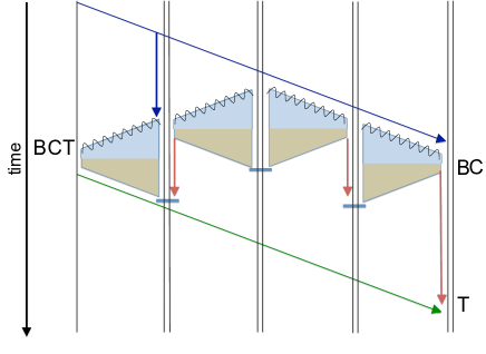
(a) Butterfly links, ridge fold timing

(b) Butterfly links, valley fold timing, Bell matched

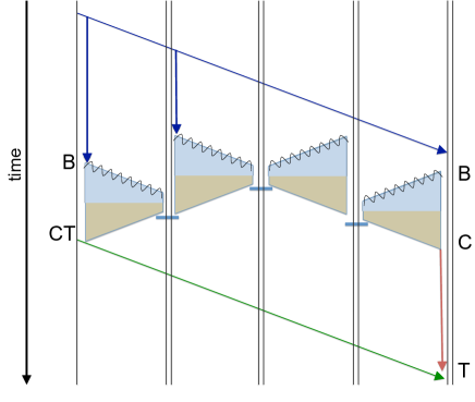
(c) Inverted butterfly, Bell matched

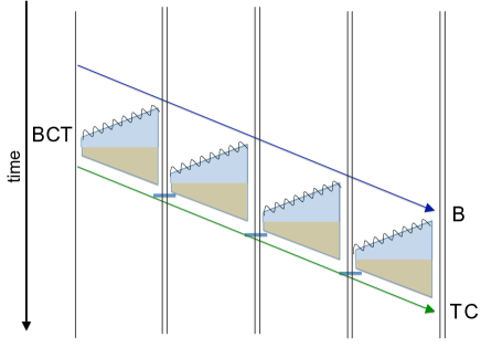
(d) Reverse propagation, forward triggered

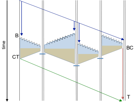
(e) Mixed direction path, optimized timing

Figure 4: Other link and timing patterns. (a) “Ridge fold” timing on butterfly link arrangement, with operation initiated from the midpoint of the path. The second Pareto condition is violated because the middle two hops start and end with two matching red arrows. (b) The same hardware configuration with “valley fold” timing created by matching Bell measurements, achieving optimality for B class and Pareto optimality for C and T classes. (c) Inverted (inside out) butterfly, with Bell matched timing. (d) Timing for counter-link propagation, with all of the links transmitting right to left to teleportation propagating left to right. This is the only path achieving zero path buffering for all three classes. (e) Mixed direction path using the matched Bell timing pattern, optimal for all three classes.

Path prop/
timing pattern	Matched?	$T^{P}_{B},T^{P}_{C}$	B,Copt?	$T^{P}_{T}$	Topt?	$T^{H}_{B}$	$T^{H}_{C},T^{H}_{T}$	Buffering
Forward
flat	N	$T_{E}-t_{1}$	N	$2T_{E}$	P	$2T_{E}-2t_{1}$	$2T_{E}$	distributed, heavy at right end point
forward	N	$2T_{E}-2t_{h}$	N	$2T_{E}$	P	$2T_{E}-2t_{1}$	$2T_{E}$	evenly distributed
uphill	Y	0	Y	$2T_{E}$	P	$2T_{E}-2t_{1}$	$2T_{E}$	all at right end point
Butterfly
ridge fold	N	$2T_{E}-2t_{\lfloor h/2\rfloor}-2t_{\lfloor h/2\rfloor+1}$	N	$\approx 3T_{E}$	N	$2T_{E}$	$2T_{E}$	distributed, heavy at right end point
valley fold	Y	0	Y	$T_{E}$	P	$2T_{E}$	$2T_{E}$	all at right end point
Inverted B’fly
ridge fold	Y	0	Y	$T_{E}$	P	$2T_{E}-2t_{1}-2t_{h}$	$2T_{E}$	all at right end point
Reverse
forward	Y	0	Y	0	Y	$2T_{E}-2t_{h}$	$2T_{E}$	none
Mixed
Bell matched	Y	0	Y	$T_{P}+\sum_{j}\tau_{j}$	P	$\leq 2T_{E}$	$2T_{E}$	all at right end point

Table 4: Path timing patterns. “Matched?” indicates whether the Bell measurement timings are matched. “opt?” indicates whether the timing pattern is Pauli optimal for that path and class of applications. “P” indicates that the pattern is one point on a Pareto optimal frontier with more than one point. “Buffering” describes the location of Pauli waits, if any.

IV Success Probability and Resource Requirements

The analysis presented here focuses on the high success probability and high success probability (extended) regimes noted in Tab. 3. Let us now make the boundaries between the probability regimes more concrete. In order to achieve deterministic, minimal timing over a path of $h$ hops, we want a high probability of all of the hops succeeding in building enough entanglement. Let the probability $P_{p}$ be the probability that the entire path cascades successfully end to end on a given trial, and $P_{s}$ be the probability that a single hop successfully cascades. Obviously, $P_{p}=(P_{s})^{h}$ for homogeneous hops, or

$$P_{p}=\prod_{j=1}^{h}P_{s}(j)$$ (17)

for heterogeneous hops; here, we will assume homogeneous. If we assume $h=50$ (long enough to cover 1,000km at 20km/hop), for $P_{s}=0.99$, we find $P_{p}\sim 0.6$.

IV.1 Asynchronous/Cascade Probability Boundary

How many transmitters $N_{T}$ do we need in each node to achieve $P_{s}=0.99$? We need at least $n$ successful entanglements in one burst, where $n$ is the block size we need for error correction (or $d$ for the surface code). The mean number of successful entanglements is $N_{r}=P_{r}N_{T}$. To guarantee that

$$P_{s}=P(N_{r}\geq n)=1-\sum_{j=0}^{n}{N_{T}\choose j}P_{r}^{j}(1-P_{r})^{N_{T}-j}\geq 0.99,$$ (18)

for $P_{r}=0.01$ and $n=7$ (as in the Steane [[7,1,3]] code steane96:_qec ), we must have $N_{T}\geq 1460$, a rather substantial overhead. The ratio is similar for $0.001<P_{r}<0.1$ for the 7-qubit code, and somewhat better for the [[23,1,7]] Golay code PhysRevA.79.032325 . We can say roughly, then, that the lower bound for the “high entanglement probability” regime is $P_{r}\sim 2n/N_{T}$. Above this level, we can coordinate the activities on links to create an efficient path, as discussed in this article.

IV.2 Cascade Generic/Direct Transmission Probability Boundary

Likewise, we can calculate the upper bound for “high probability”, the transition to direct transmission of quantum data, without first building generic states such as Bell states. Although certain cases allow reconstruction with less than half of the physical qubits comprising a logically encoded state silva2004erasure , in general, the no-cloning theorem shows that we need to receive more than half, that is,

$$P_{s}=P(N_{r}\geq\lceil h/2\rceil)=1-\sum_{j=0}^{\lfloor h/2\rfloor}{n\choose j}P_{r}^{j}(1-P_{r})^{n-j}.$$ (19)

For direct transmission we need $P_{s}$ to be substantially higher than 0.99, e.g., $P_{s}=0.999$ or better when transporting valuable quantum data, perhaps as high as $1-10^{-15}$ for some forms of distributed quantum computation Chien:2015:FOU:2810396.2700248 ; van-meter14:_quantum_networking . For the seven-qubit Steane code and $P_{s}=0.999$, we would need $P_{r}\geq 0.93$, whereas for the 23-qubit Golay code we would need $P_{r}\geq 0.79$. The value of $\alpha$ in Tab. 3 therefore is highly code dependent, but for our purposes here can be considered to be in the range $0.8\leq\alpha\leq 0.95$. We call the region $0.5<P_{r}\leq\alpha$ the “high probability (extended)” regime, and in this regime our timing analysis still applies.

Direct transmission requires that the polarity of the links correspond to the desired direction of propagation along the entire path, or equivalently that the links are duplex. When this condition does not hold, operational procedures will instead fall back to the procedures and timing behavior discussed in this paper.

V Discussion

Muralidharan et al. divided quantum repeater architectures into three generations muralidharan15:_ultrafast-generations :

1. First generation: using bidirectional entanglement purification (2-EPP) and acknowledged (heralded) entanglement generation (known as AEC or HEG);

2. Second generation: using unidirectional entanglement purification (1-EPP), e.g. based on error correcting codes, and acknowledged (sometimes called heralded) entanglement generation (known as AEC or HEG); and

3. Third generation: using unidirectional entanglement purification (1-EPP), e.g. based on error correcting codes, and unacknowledged but heralded (without acknowledgement to partner) loss error management, allowing direct transmission of states.

Our analysis differs in several respects: (1) we discuss the three application classes B, C, and T, whereas earlier analysis focused on the QKD application or equivalent Bell inequality violation tests; (2) we focus on optimizing the timing pattern; (3) we explicitly consider heterogeneity in paths; and (4) we study the impact of the link polarity. Primarily, our contribution can be considered to be optimization of 2G repeater timing, but the B/C/T distinction allows us to also further subdivide 2G repeaters into path-optimizable and non-path-optimizable subclasses.

Even for the relatively simple useage of the Steane code, and assuming improvement to around 1% entanglement success probability, the resource requirements for achieving this cascaded operation are substantial. 1,400 transmitter qubits is likely to remain well out of reach in actual implementation for a number of years. Moreover, with 1,400 transmitters, the expected number of successful entanglements would be $\sim 14$, enough to create two Steane transfers. The more likely operational approach, therefore, would be to continue asynchronous operation in order to take advantage of the extra resources.

Once entanglement success probability reaches several percent, the optimizations presented here will guide network protocols and operations to substantially improved performance by reducing buffer memory needs (slightly at low $P_{r}$, substantially at high $P_{r}$), and by reducing memory decoherence. Following the guidelines here, the location of buffer memory consumed can be adjusted along a Pareto optimal frontier, providing operational flexiblity. With end-to-end latencies of around $T_{E}\approx 100$msec between some locations on the globe, the reduction from $5T_{E}$ (worst case for ridge fold timing on butterfly links) to $2T_{E}$ in the best case can save hundreds of milliseconds of memory decoherence time in a Quantum Internet.

References

- [1] A.K. Ekert. Quantum cryptography based on Bell’s theorem. Physical Review Letters, 67(6):661–663, 1991.
- [2] Richard Jozsa, Danial S. Abrams, Jonathan P. Dowling, and Colin P. Williams. Jozsa et al. reply:. Phys. Rev. Lett., 87:129802, Aug 2001.
- [3] I.L. Chuang. Quantum algorithm for distributed clock synchronization. Physical Review Letters, 85(9):2006–2009, 2000.
- [4] Daniel Gottesman, Thomas Jennewein, and Sarah Croke. Longer-baseline telescopes using quantum repeaters. Phys. Rev. Lett., 109:070503, Aug 2012.
- [5] Claude Creṕeau, Daniel Gottesman, and Adam Smith. Secure multi-party quantum computation. In Proc. Symposium on Theory of Computing. ACM, 2002.
- [6] Anne Broadbent, Joseph Fitzsimons, and Elham Kashefi. Universal blind quantum computation. In Foundations of Computer Science, 2009. FOCS’09. 50th Annual IEEE Symposium on, pages 517–526. IEEE, 2009.
- [7] Seiichiro Tani, Hirotada Kobayashi, and Keiji Matsumoto. Exact quantum algorithms for the leader election problem. ACM Trans. Comput. Theory, 4(1):1:1–1:24, March 2012.
- [8] Charles H. Bennett, David P. DiVincenzo, John A. Smolin, and William K. Wootters. Mixed-state entanglement and quantum error correction. Physical Review A, 54(5):3824–3851, Nov 1996.
- [9] W. Dür, H.-J. Briegel, J. I. Cirac, and P. Zoller. Quantum repeaters based on entanglement purification. Physical Review A, 59(1):169–181, Jan 1999.
- [10] E. Knill and R. Laflamme. Concatenated quantum codes. http://arXiv.org/quant-ph/9608012, August 1996.
- [11] Liang Jiang, J. M. Taylor, Kae Nemoto, W. J. Munro, Rodney Van Meter, and M. D. Lukin. Quantum repeater with encoding. Phys. Rev. A, 79(3):032325, Mar 2009.
- [12] Austin G. Fowler, David S. Wang, Charles D. Hill, Thaddeus D. Ladd, Rodney Van Meter, and Lloyd C. L. Hollenberg. Surface code quantum communication. Phys. Rev. Lett., 104(18):180503, May 2010.
- [13] Sreraman Muralidharan and Liang Jiang. Potential for ultrafast quantum communication. SPIE Newsroom, 2015.
- [14] H. J. Kimble. The quantum Internet. Nature, 453:1023–1030, June 2008.
- [15] Rodney Van Meter. Quantum Networking. Wiley-ISTE, April 2014.
- [16] Shota Nagayama, Byung-Soo Choi, Simon Devitt, Shigeya Suzuki, and Rodney Van Meter. Interoperability in encoded quantum repeater networks. Phys. Rev. A, 93:042338, Apr 2016.
- [17] Reinhold A. Bertlmann, Heide Narnhofer, and Walter Thirring. Time-ordering dependence of measurements in teleportation. The European Physical Journal D, 67(3), 2013.
- [18] C. K. Hong, Z. Y. Ou, and L. Mandel. Measurement of subpicosecond time intervals between two photons by interference. Phys. Rev. Lett., 59:2044–2046, Nov 1987.
- [19] C. Cabrillo, J. I. Cirac, P. García-Fernández, and P. Zoller. Creation of entangled states of distant atoms by interference. Phys. Rev. A, 59(2):1025–1033, Feb 1999.
- [20] L.M. Duan, M.D. Lukin, J.I. Cirac, and P. Zoller. Long-distance quantum communication with atomic ensembles and linear optics. Nature, 414:413–418, 2001.
- [21] L.-M. Duan and C. Monroe. Colloquium : Quantum networks with trapped ions. Rev. Mod. Phys., 82:1209–1224, Apr 2010.
- [22] T. P. Spiller, Kae Nemoto, Samuel L. Braunstein, W. J. Munro, P. van Loock, and G. J. Milburn. Quantum computation by communication. New Journal of Physics, 8:30, February 2006.
- [23] D Hucul, IV Inlek, G Vittorini, C Crocker, S Debnath, SM Clark, and C Monroe. Modular entanglement of atomic qubits using photons and phonons. Nature Physics, 11:37–42, 2014.
- [24] A. Sipahigil, M. L. Goldman, E. Togan, Y. Chu, M. Markham, D. J. Twitchen, A. S. Zibrov, A. Kubanek, and M. D. Lukin. Quantum interference of single photons from remote nitrogen-vacancy centers in diamond. Phys. Rev. Lett., 108:143601, Apr 2012.
- [25] H Bernien, B Hensen, W Pfaff, G Koolstra, MS Blok, L Robledo, TH Taminiau, M Markham, DJ Twitchen, L Childress, et al. Heralded entanglement between solid-state qubits separated by three metres. Nature, 497(7447):86–90, 2013.
- [26] Cody Jones, Danny Kim, Matthew T Rakher, Paul G Kwiat, and Thaddeus D Ladd. Design and analysis of communication protocols for quantum repeater networks. arXiv preprint arXiv:1505.01536, 2015.
- [27] M. Aspelmeyer, T. Jennewein, M. Pfennigbauer, WR Leeb, and A. Zeilinger. Long-distance quantum communication with entangled photons using satellites. Selected Topics in Quantum Electronics, IEEE Journal of, 9(6):1541–1551, 2003.
- [28] K. Boone, J.-P. Bourgoin, E. Meyer-Scott, K. Heshami, T. Jennewein, and C. Simon. Entanglement over global distances via quantum repeaters with satellite links. Phys. Rev. A, 91:052325, May 2015.
- [29] Cheng-Zhi Peng, Tao Yang, Xiao-Hui Bao, Jun Zhang, Xian-Min Jin, Fa-Yong Feng, Bin Yang, Jian Yang, Juan Yin, Qiang Zhang, Nan Li, Bao-Li Tian, and Jian-Wei Pan. Experimental free-space distribution of entangled photon pairs over 13 km: Towards satellite-based global quantum communication. Phys. Rev. Lett., 94:150501, Apr 2005.
- [30] W. K. Wootters and W. H. Zurek. A single quantum cannot be cloned. Nature, 299:802–803, October 1982.
- [31] Charles H. Bennett, David P. DiVincenzo, and John A. Smolin. Capacities of quantum erasure channels. Phys. Rev. Lett., 78:3217–3220, Apr 1997.
- [32] Rodney Van Meter, Thaddeus D. Ladd, W. J. Munro, and Kae Nemoto. System design for a long-line quantum repeater. IEEE/ACM Transactions on Networking, 17(3):1002–1013, June 2009.
- [33] Luciano Aparicio, Rodney Van Meter, and Hiroshi Esaki. Protocol design for quantum repeater networks. In Proc. Asian Internet Engineering Conference, November 2011.
- [34] C.H. Bennett, G. Brassard, S. Popescu, B. Schumacher, J.A. Smolin, and W.K. Wootters. Purification of noisy entanglement and faithful teleportation via noisy channels. Physical Review Letters, 76(5):722–725, 1996.
- [35] David Deutsch, Artur Ekert, Richard Jozsa, Chiara Macchiavello, Sandu Popescu, and Anna Sanpera. Quantum privacy amplification and the security of quantum cryptography over noisy channels. Phys. Rev. Lett., 77(13):2818–2821, Sep 1996.
- [36] M. Żukowski, A. Zeilinger, M. A. Horne, and A. K. Ekert. “Event-ready-detectors” Bell experiment via entanglement swapping. Phys. Rev. Lett., 71:4287–4290, Dec 1993.
- [37] H.-J. Briegel, W. Dür, J.I. Cirac, and P. Zoller. Quantum repeaters: the role of imperfect local operations in quantum communication. Physical Review Letters, 81:5932–5935, 1998.
- [38] Rodney Van Meter, Takahiko Satoh, Thaddeus D. Ladd, William J. Munro, and Kae Nemoto. Path selection for quantum repeater networks. Networking Science, 3(1):82–95, 2013.
- [39] WJ Munro, KA Harrison, AM Stephens, SJ Devitt, and K. Nemoto. From quantum multiplexing to high-performance quantum networking. Nature Photonics, 4:792–796, 2010.
- [40] Andrew Steane. Error correcting codes in quantum theory. Physical Review Letters, 77:793–797, 1996.
- [41] Marcus da Silva. Erasure thresholds for efficient linear optics quantum computation. Master’s thesis, University of Waterloo, 2004.
- [42] Chia-Hung Chien, Rodney Van Meter, and Sy-Yen Kuo. Fault-tolerant operations for universal blind quantum computation. J. Emerg. Technol. Comput. Syst., 12(1):9:1–9:26, August 2015.