Grand canonical electronic density-functional theory:
algorithms and applications to electrochemistry

Abstract

First-principles calculations combining density-functional theory and continuum solvation models enable realistic theoretical modeling and design of electrochemical systems. When a reaction proceeds in such systems, the number of electrons in the portion of the system treated quantum mechanically changes continuously, with a balancing charge appearing in the continuum electrolyte. A grand-canonical ensemble of electrons at a chemical potential set by the electrode potential is therefore the ideal description of such systems that directly mimics the experimental condition. We present two distinct algorithms, a self-consistent field method (GC-SCF) and a direct variational free energy minimization method using auxiliary Hamiltonians (GC-AuxH), to solve the Kohn-Sham equations of electronic density-functional theory directly in the grand canonical ensemble at fixed potential. Both methods substantially improve performance compared to a sequence of conventional fixed-number calculations targeting the desired potential, with the GC-AuxH method additionally exhibiting reliable and smooth exponential convergence of the grand free energy. Finally, we apply grand-canonical DFT to the under-potential deposition of copper on platinum from chloride-containing electrolytes and show that chloride desorption, not partial copper monolayer formation, is responsible for the second voltammetric peak.

Density-functional theory (DFT) enables theoretical elucidation of reaction mechanisms at complex catalyst surfaces, making it now possible to design efficient heterogeneous catalysts for various industrial applications from first principles, for example for high-temperature gas-phase transformation of hydrocarbons to a variety of valuable chemical products.Cheng and Goddard III (2015); Cheng, Goddard III, and Fu (2014) The extension of this predictive power to electrocatalysis would be highly valuable for an even broader class of technological problems, including a cornerstone of future technology for renewable energy: converting solar energy to chemical fuels by electrochemical water splitting and carbon dioxide reduction.Walter et al. (2010) Accurately describing electrochemical phenomena, however, presents two additional challenges.

First, the electrolyte, typically consisting of ions in a liquid solvent, strongly affects the energetics of structures and reactions at the interface. Treating liquids directly in DFT requires expensive molecular dynamics to sample the thermodynamic phase space of atomic configurations. Historically, a number of continuum solvation models that empirically capture liquid effects have enabled theoretical design of liquid-phase catalysts.Marenich, Cramer, and Truhlar (2009); Tomasi, Mennucci, and Cammi (2005) More recently, empirical solvation models suitable for solid-liquid interfaces,Andreussi, Dabo, and Marzari (2012); Gunceler et al. (2013); Matthew et al. (2014) joint density-functional theory (JDFT) for efficiently treating liquids with atomic-scale structure,Petrosyan et al. (2007) and minimally-empirical solvation models derived from JDFT,Sundararaman et al. (2015); Sundararaman and Goddard III (2015) have made great strides towards reliable yet efficient treatment of electrochemical systems.

Second, electrons can flow in and out of the electrode as electrochemical reactions proceed. Changes in electronic charge of electrode surfaces and adsorbates can be especially important because the electrolyte stabilizes charged configurations with a counter charge from the ionic response. For example, reduction of formic acid on platinum at experimentally relevant potentials is dominated by formate ions rather than neutral molecules at the surface.Schwarz et al. (2015) Proton adsorption on stepped and polycrystalline surfaces involves displacing oxidatively-adsorbed water at relevant potentials, resulting in non-integer charge transfers and an anomalous pH dependence deviating from the Nernst equation.Schwarz et al. (2016)

Accounting for the electrolyte response using our solvation models,Sundararaman and Goddard III (2015); Matthew et al. (2014) and adjusting the electron number to match experimentally relevant electrode potentials, realistic predictions of electrochemical reaction mechanisms have now become possible.Goodpaster, Bell, and Head-Gordon (2016) In particular, application of this methodology to the reduction of CO on Cu(111) predicts onset potentials for methane and ethene formation with 0.05 V accuracy in comparison to experiment, for a wide range of pH varying from 1 to 12.Xiao et al. (2016) However, conventional DFT software and algorithms are optimized for solving the quantum-mechanical problem at fixed electron number, requiring extra work (both manual and computational) to calculate properties for a specified electrode potential.

Electric potentials and fields play an important role in fields besides than electrochemistry. Density-functional theory approaches accounting for electric potential have been developed in special cases for field emission from metal surfaces using a jellium model,Gohda et al. (2000) and for calculating capacitance in metal-insulator-metalStengel and Spaldin (2007); Kasamatsu, Watanabe, and Han (2011) and carbon nanotube systems.Uchida et al. (2007) Calculating non-equilibrium transport of electrons in nanoscale systems also requires accounting for potential difference between reservoirs in a DFT calculation.Brandbyge et al. (2002) First-principles molecular dynamics approaches have been developed to emulate fixed potential using fluctuating numbers of electrons between time steps.Bonnet et al. (2012) However, in all these cases, each involved self-consistent DFT calculation contains a fixed number of electrons and is carried out using a conventional canonical-ensemble algorithm.

This paper introduces algorithms for grand canonical DFT, where electron number adjusts automatically to target a specified electron chemical potential (related to electrode potential), thereby enabling efficient and intuitive first-principles treatment of electrochemical phenomena. Section I summarizes the theoretical background of first-principles electrochemistry using JDFT and continuum solvation models, and sets up the fundamental basis of grand-canonical DFT. Then, section II introduces the modifications necessary to make two distinct classes of DFT algorithms, the self-consistent field (GC-SCF) method and the variational free energy minimization using auxiliary Hamiltonians (GC-AuxH), directly converge the grand free energy of electrons at fixed potential. Sections III.2 and III.3 establish the algorithm parameter(s) that optimize the iterative convergence of the GC-SCF and GC-AuxH methods respectively, while section III.4 compares the performance of these algorithms for a number of prototypical electrochemical systems. Finally, section III.5 demonstrates the utility of grand canonical DFT by solving an electrochemical mystery: the identity of the second voltammetric peak in the under-potential deposition (UPD) of copper on platinum in chloride-containing electrolytes.

I Theory

I.1 Background: electronic density functional theory

The exact Helmholtz free energy $A$ of a system of interacting electrons in an external potential $V(\mathbf{r})$ at a finite temperature $T$ satisfies the Hohenberg-Kohn-Mermin variational theoremHohenberg and Kohn (1964); Mermin (1965)

$$A=\min_{n(\mathbf{r})}\left(A_{\textrm{HKM}}^{T}[n(\mathbf{r})]+\int d\mathbf{r}V(\mathbf{r})n(\mathbf{r})\right),$$ (1)

where $A_{\textrm{HKM}}^{T}$ is a universal functional that depends only on the electron density $n(\mathbf{r})$ (and temperature), and not on the external potential. However, constructing approximations for this unknown universal functional that accurately capture the energies and geometries of chemical bonds in terms of the density alone is extremely challenging, partly because the quantum mechanics of the electrons is completely implicit in $A_{\textrm{HKM}}[n]$ (dropping the $T$ labels here onward for notational simplicity; all the functionals below depend on temperature).

Most practical approximations in electronic density-functional theory follow the Kohn-Sham approachKohn and Sham (1965) that includes the exact free energy of a non-interacting system of electrons with the same density $n(\mathbf{r})$. The universal functional is typically split as

$$A_{\textrm{HKM}}[n]=A_{\textrm{ni}}[n]+\underbrace{\int d\mathbf{r}\int d\mathbf{r}^{\prime}\frac{n(\mathbf{r})n(\mathbf{r}^{\prime})}{2|\mathbf{r}-\mathbf{r}^{\prime}|}}_{E_{H}[n]}+E_{\textrm{XC}}[n],$$ (2)

where $A_{\textrm{ni}}[n]$ is the non-interacting free energy (which we describe in detail below), the second ‘Hartree’ term $E_{H}[n]$ is the mean-field Coulomb interaction between electrons (using atomic units $e,m_{e},\hbar,k_{B}=1$ throughout), and the final ‘exchange-correlation’ term $E_{\textrm{XC}}[n]$ captures the remainder which is not known and must hence be approximated. The exact free energy of non-interacting electrons is

$$A_{\textrm{ni}}[n]=\min_{\mbox{\scriptsize$\begin{array}[]{c}\{\psi_{i}(\mathbf{r}),f_{i}\}\\ \rightarrow n(\mathbf{r})\end{array}$}}\sum_{i}\bigg{(}\underbrace{\frac{f_{i}}{2}\int d\mathbf{r}|\nabla\psi_{i}(\mathbf{r})|^{2}}_{\textrm{Kinetic}}\\ -T\underbrace{S(f_{i})}_{\textrm{Entropy}}\bigg{)},$$ (3)

which includes the kinetic energy and entropy contributions of a set of orthonormal single-particle orbitals $\psi_{i}(\mathbf{r})$ with occupation factors $f_{i}\in[0,1]$. Above, the single-particle entropy function is $S(f)=-f\log f-(1-f)\log(1-f)$. Note that we let the orbital index $i$ include spin degrees of freedom as well, and therefore do not introduce factors of 2 for spin degeneracy. For notational convenience, we also let $i$ include Bloch wave-vectors in the Brillouin zone (in addition to spin and band indices) for periodic systems.

The minimization in (3) is constrained such that the density of the non-interacting system

$$\sum_{i}f_{i}|\psi_{i}(\mathbf{r})|^{2}=n(\mathbf{r}),$$ (4)

the density of the real interacting system. Performing this minimization with Lagrange multipliers $V_{\textrm{KS}}(\mathbf{r})$ (the Kohn-Sham potential) to enforce the density constraint and $\varepsilon_{i}$ (Kohn-Sham eigenvalues) to enforce orbital normalization constraints, results in a set of single-particle Schrödinger-like equations

$$-\frac{\nabla^{2}}{2}\psi_{i}(\mathbf{r})+V_{\textrm{KS}}(\mathbf{r})\psi_{i}(\mathbf{r})=\varepsilon_{i}\psi_{i}(\mathbf{r})$$ (5)

for stationarity with respect to $\psi_{i}(\mathbf{r})$, and the Fermi occupation condition

$$f_{i}=\frac{1}{1+\exp\frac{\varepsilon_{i}-\mu}{T}}$$ (6)

for stationarity with respect to $f_{i}$. Here, the electron chemical potential $\mu$ appears as a Lagrange multiplier to enforce the electron number constraint, and is chosen so that $\sum f_{i}=N$, the number of electrons in the system.

Optimizing the total free energy functional (1) with $A_{\textrm{HKM}}[n]$ implemented by (2,3) then yields the stationarity condition with respect to electron density,

$$V_{\textrm{KS}}[n](\mathbf{r})=V(\mathbf{r})+\frac{\delta}{\delta n(\mathbf{r})}\left(E_{H}[n]+E_{\textrm{XC}}[n]\right).$$ (7)

Conventional density-functional theory calculations then amount to self-consistently solving the Kohn-Sham equations (5) along with (7), coupled via the electron density constraint (4).

The Kohn-Sham potential is arbitrary up to an overall additive constant: changing this constant introduces a rigid shift in the eigenvalues $\epsilon_{i}$ and the electron chemical potential $\mu$, but does not affect the occupations $f_{i}$, electron density or free energy. For finite systems (of any charge) and for neutral systems that are infinitely periodic in one or two directions, this arbitrariness can be eliminated by requiring that the potential vanishes infinitely far away from the system, giving meaning to the absolute values of $\mu$ and $\epsilon_{i}$ as being referenced to ‘zero at infinity’. However, for materials that are infinite in all three dimensions, such as periodic crystalline solids, there is no analogous natural choice for the zero of potential, making the absolute reference for $\mu$ and $\epsilon_{i}$ meaningless.

More importantly, for systems that are periodic in one, two or all three directions, the net charge per unit cell must be zero, otherwise the energy per unit cell becomes infinite. In terms of a finite system size $L$ and then taking the limit $L\rightarrow\infty$, the energy per unit cell of a system with net charge per unit cell diverges $\propto\ln L$ for one periodic direction, $\propto L$ for two periodic directions and $\propto L^{2}$ for three periodic directions. Therefore, the number of electrons per unit cell is physically constrained to keep the unit cell neutral in systems with any periodicity, and only finite systems (like molecules and ions) have number of electrons as a degree of freedom.

I.2 Electrochemistry with joint density-functional theory

For describing electrochemical systems and electrocatalytic mechanisms, we are typically interested in adsorbed species in a solid-electrolyte interface which exchange electrons with the solid (electrode). In these systems, the solid surface, which we would describe in a density-functional calculation as a slab periodic in two directions, does have a net charge per unit cell that depends on the electrode potential. In contrast to the discussion at the end of the previous section, this is physically possible (i.e. has a finite energy) because the electrolyte contains mobile ions that respond by locally increasing the concentration of ions of opposite charge near the surface, thereby neutralizing the unit cell. (The charge per unit areas of the electrode and electrolyte are equal and opposite.)

Next to an electrolyte, the charge of a partially-periodic system (one-dimensional ‘wires’ or two-dimensional ‘slabs’) is no longer constrained, allowing the number of electrons to vary. Now, the absolute reference for the electron chemical potential $\mu$ does become physically meaningful, and $\mu$ now corresponds to the electrode potential that controls the number of electrons in the electrode.

However, treating electrochemical systems using electronic density-functional theory alone is extremely challenging for a variety of reasons. First, treating liquids requires a statistical average over a large number of atomic configurations to integrate over thermodynamic phase space. For this, techniques such as molecular dynamics typically require calculations of at least $10^{4}-10^{5}$ atomic configurations (instead of just one for a solid). Second, such calculations require a large number of liquid molecules to minimize finite size errors in the molecular dynamics. For example, for electrolytes with a realistic ionic concentration of 0.1 M, there is on average one ion for a few hundred solvent molecules. Making statistical errors in the ion number manageable in such calculations therefore requires $>10^{3}$ solvent molecules with $>10^{4}$ electrons, contrasted with a typical $10-100$ atoms with $100-10^{3}$ electrons in the electrode slab + adsorbate of interest. Combined, these factors make density-functional molecular dynamics simulations of electrochemical systems prohibitively expensive computationally, in additional to being difficult to set up and analyze.

A viable alternative to the above direct approach is to employ joint density-functional theoryPetrosyan et al. (2007) (JDFT), a variational theorem akin to the Hohenberg-Kohn theorem that makes it possible to describe the free energy of a solvated system in terms of the electron density $n(\mathbf{r})$ for the solute and in terms of a set of nuclear densities $\{N_{\alpha}(\mathbf{r})\}$ (where $\alpha$ indexes nuclear species) of the solvent (or electrolyte). Specifically, the equilibrium free energy of the combined solute and solvent systems minimizes

$$A=\min_{n(\mathbf{r}),\{N_{\alpha}(\mathbf{r})\}}\bigg{(}\tilde{A}_{\textrm{JDFT}}[n(\mathbf{r}),\{N_{\alpha}(\mathbf{r})\}]\\ +\int d\mathbf{r}V(\mathbf{r})n(\mathbf{r})+\sum_{\alpha}\int d\mathbf{r}V_{\alpha}(\mathbf{r})N_{\alpha}(\mathbf{r})\bigg{)},$$ (8)

where $V(\mathbf{r})$ is the external electron potential, $V_{\alpha}(\mathbf{r})$ is the external potential on the liquid nuclei and $A_{\textrm{JDFT}}$ is a universal functional independent of these external potentials. Separating out the Hohenberg-Kohn electronic density functional $A_{\textrm{HK}}[n]$ for the solute, the total free energy is

$$\tilde{A}_{\textrm{JDFT}}[n,\{N_{\alpha}\}]=\underbrace{A_{\textrm{HKM}}[n]}_{\textrm{electronic}}+\underbrace{\tilde{A}_{\textrm{diel}}[n,\{N_{\alpha}\}]}_{\textrm{solvation}}.$$ (9)

In practice, the functional $A_{\textrm{diel}}$, much like $A_{\textrm{HKM}}$, is unknown and needs to be approximated. Importantly, the liquid is now described directly in terms of its average density rather than individual configurations, and the expensive quantum-mechanical theory of the electrons is restricted to the solute alone, thereby addressing both the sampling and system-size problems that make density-functional molecular dynamics prohibitively expensive.

Typically, we are interested in a situation where the external potentials on the liquid are zero, and the liquid only interacts with itself, and with the electrons and nuclei of the solute. In this situation, we can perform the optimization over liquid densities and define the implicit functional $A_{\textrm{JDFT}}[n]=A_{\textrm{HKM}}[n]+A_{\textrm{diel}}[n]$ where we define $A_{X}[n]\equiv\min_{\{N_{\alpha}(\mathbf{r})\}}\tilde{A}_{X}[n(\mathbf{r}),\{N_{\alpha}(\mathbf{r})\}]$ for $X$ = JDFT and $X$ = diel. We will work with these reduced functionals below for simplicity.

The framework of joint density-functional theory encompasses an entire hierarchy of solvation theories. Further separating the solvation term $A_{\textrm{diel}}$ into a classical density functional for the liquidSundararaman, Letchworth-Weaver, and Arias (2012); Sundararaman and Arias (2014); Sundararaman, Letchworth-Weaver, and Arias (2014) and an electron-liquid interaction functional, unlocks the full potential of JDFT to describe atomic-scale structure in the liquid without statistical sampling. Starting from ‘full-JDFT’ and performing perturbation theory for linear-response of the liquid results in the non-empirical SaLSA solvation modelSundararaman et al. (2015) which continues to capture the atomic-scale nonlocality in the liquid response and introduces no fit parameters for the electric response of the solvent.

At the simplest end of the JDFT hierarchy, are continuum solvation models that neglect the nonlocality of the liquid response and replace it by that of an empirically-determined dielectric cavity (optionally with Debye screening due to electrolytes). This includes our recent CANDLE solvation modelSundararaman and Goddard III (2015) that builds on the stability of SaLSA for highly polar systems, and earlier solvation models suitable for molecules and less-polar systems such as our GLSSA13 modelGunceler et al. (2013) (or its equivalent, VASPsolMatthew et al. (2014)) and the comparable Self-Consistent Continuum Solvation (SCCS) model.Andreussi, Dabo, and Marzari (2012); Dupont, Andreussi, and Marzari (2013) Even the traditional quantum-chemistry finite-system solvation models such as the PCM seriesTomasi, Mennucci, and Cammi (2005) and the SMx seriesMarenich, Cramer, and Truhlar (2009) can be mapped on to this class of solvation models.

For simplicity, we will work here with this simplest class of continuum solvation models. The theoretical considerations and algorithms in this work focus primarily the electronic density-functional theory component, are largely agnostic to the internals of the solvation model and therefore straightforwardly generalize up the JDFT hierarchy to the more detailed and complex solvation theories. Essentially, all the simple electron-density-based continuum solvation modelsSundararaman and Goddard III (2015); Gunceler et al. (2013); Matthew et al. (2014); Andreussi, Dabo, and Marzari (2012) can be summarized abstractly asGunceler et al. (2013); Sundararaman et al. (2015)

$$A_{\textrm{diel}}[n(\mathbf{r})]=\int d\mathbf{r}\rho_{\textrm{el}}(\mathbf{r})\frac{(\hat{K}^{-1}-\hat{\chi})^{-1}-\hat{K}}{2}\rho_{\textrm{el}}(\mathbf{r})+A_{\textrm{cav}}[s].$$ (10)

Here, the first term is the electrostatic solute-solvent interaction energy given by the difference between the solvent-screened Coulomb interaction and the bare Coulomb interaction $\hat{K}$ of the total solute charge density, $\rho_{\textrm{el}}(\mathbf{r})=n(\mathbf{r})+\rho_{\textrm{nuc}}(\mathbf{r})$, where $\rho_{\textrm{nuc}}(\mathbf{r})$ is the solute nuclear charge density. The screened Coulomb interaction term above is expressed in terms of the bare Coulomb interaction $\hat{K}$ and the solvent susceptibility operator $\hat{\chi}$, defined for the local-response models by

$$\hat{\chi}\cdot\phi(\mathbf{r})\equiv\underbrace{\nabla\cdot\left(\frac{\epsilon_{b}-1}{4\pi}s(\mathbf{r})\nabla\phi(\mathbf{r})\right)}_{\textrm{Dielectric}}-\underbrace{\frac{\kappa^{2}}{4\pi}s(\mathbf{r})\phi(\mathbf{r})}_{\textrm{Ionic}}.$$ (11)

Here, $\epsilon_{b}$ is the bulk dielectric constant of the solvent and $\kappa=\sqrt{4\pi\sum_{i}N_{i}Z_{i}^{2}/T}$ is the inverse Debye screening length in vacuum of a set of ionic species of charge $Z_{i}$ with concentrations $N_{i}$ (the net inverse Debye screening length in the presence of the background dielectric is $\kappa/\sqrt{\epsilon_{b}}$). The cavity shape function $s(\mathbf{r})$ modulates the dielectric and ion response, and varies from zero in the solute region (no solvent present) to unity in the solvent at full bulk density. Finally, the second term of (10), $A_{\textrm{cav}}$, empirically captures effects beyond mean-field electrostatics, such as the free energy of cavity formation in the liquid and dispersion interactions between the solute and solvent.Sundararaman, Gunceler, and Arias (2014) Different solvation models at this level of the hierarchy only differ in the details of how $s(\mathbf{r})$ is determined from the electron density (or even from atomic positions and fit radii for the PCMTomasi, Mennucci, and Cammi (2005) and SMxMarenich, Cramer, and Truhlar (2009) solvation models), and in the details of $A_{\textrm{cav}}$.

In practice, evaluating the first term of (10) requires the calculation of $\phi(\mathbf{r})=(\hat{K}^{-1}-\hat{\chi})^{-1}\rho_{\textrm{el}}(\mathbf{r})$, which is the net electrostatic potential including screening by the solvent (and electrolyte). The second part of the first term in (10) represents the electrostatic interactions between electrons and the nuclei in vacuum which cancels corresponding terms in the vacuum DFT functional (specifically the Hartree, Ewald and long-range part of the local pseudopotential terms), so that all long-range terms that contribute to the net free energy are present in the first term of (10). Finally, substituting (11) and $\hat{K}^{-1}=-\nabla^{2}/(4\pi)$ into the definition of $\phi(\mathbf{r})$ results in the linearized Poisson-Boltzmann (modified Helmholtz) equation

$$-\nabla\cdot\left(\epsilon_{b}s(\mathbf{r})\nabla\phi(\mathbf{r})\right)+\kappa^{2}s(\mathbf{r})\phi(\mathbf{r})=4\pi\rho_{\textrm{el}}(\mathbf{r}).$$ (12)

Without ionic screening (second term of (12) above), the absolute reference for $\phi(\mathbf{r})$ is undetermined and does not contribute to the bound charge charge induced in the liquid, $\hat{\chi}\phi(\mathbf{r})$ (given by the first term of (11) alone), because $\nabla(\mathrm{constant})=0$. However, with ionic screening, a constant shift of $\phi(\mathbf{r})$ does affect the second terms of (11) and (12), producing a charge response in the liquid and making the absolute reference of the electrostatic potential $\phi(\mathbf{r})$ meaningful. In particular, integrating (12) over space yields

$$\int d\mathbf{r}\frac{\kappa^{2}}{4\pi}s(\mathbf{r})\phi(\mathbf{r})=\int\rho_{\textrm{el}}(\mathbf{r}).$$ (13)

From (11), the left hand side is the negative of the total bound charge in the liquid, while the right hand side is the total charge of the solute system. Therefore, the continuum electrolyte automatically compensates for any net charge in the solute and makes the complete system neutral. As a side effect, the absolute reference of the electrostatic potential is meaningful and automatically corresponds to ‘zero at infinity’. This happens because the Greens function of (12) is $\exp(-\kappa r/\sqrt{\epsilon_{b}})/r$ in the bulk liquid with finite $\kappa$ (instead of $1/r$), causing $\phi(\mathbf{r})$ to exponentially decay to zero outside the solute region (where $\rho_{\textrm{el}}=0$).

Ref. 30 gives a detailed version of the above discussion including rigorous proofs of the absoluteness of the reference for $\phi(\mathbf{r})$, and numerical details and algorithms for efficiently solving (12) with periodic boundary conditions in plane-wave basis DFT calculations. The result that the electrolyte neutralizes charges in the solute is true more generally, even for solvation models with nonlinearGunceler et al. (2013) and/or nonlocal response.Sundararaman et al. (2015) However, as Ref. 7 describes in detail, for the general nonlinear case, unit cell neutralization is not automatic and must be imposed using a Lagrange multiplier constraint; this Lagrange multiplier then fixes the absolute value of $\phi(\mathbf{r})$ such that it is zero at infinity.

The key conclusion of this discussion is that continuum electrolytes present two advantages. First, automatic charge neutralization implies we can perform well-defined calculations with net charge per unit cell in the solute. Second, meaningful absolute reference values for potentials implies that the electron chemical potential $\mu$ (which determines the electron occupations in (6)) is also referenced to zero at infinity. Consequently, $\mu$ is related directly to the potential $U$ of the electrode providing the electron reservoir in experiments. This potential is typically referenced to the standard hydrogen electrode (SHE), so that

$$\mu=\mu_{\textrm{SHE}}-U,$$ (14)

where $\mu_{\textrm{SHE}}$ is the absolute position of the standard hydrogen electrode relative to the vacuum level (i.e. the zero at infinity reference). Calculations can employ either the experimental estimate $\mu_{\textrm{SHE}}=-4.44$ eV to relate the absolute and relative potential scales,Trasatti (1986); Cheng and Sprik (2012) or a theoretical calibration based on the calculated and measured potentials of zero charge of solvated metal surfaces.Letchworth-Weaver and Arias (2012) The latter approach has the advantage of minimizing systematic errors in the solvation model since they cancel between the calculations used for calibration and prediction. For example, with the CANDLE solvation model we use below, the calibrated $\mu_{\textrm{SHE}}=-4.66$ eV.Sundararaman and Goddard III (2015)

I.3 Grand-canonical density-functional theory

Using joint density-functional theory of continuum solvation models to treat electrolytes as described above, we can calculate the Helmholtz free energy and electrochemical potential ($\mu$, and hence $U$) of specific microscopic configurations of adsorbates on electrode surfaces at a fixed number of electrons $N$ in the solute subsystem (electrode + adsorbates). However, in electrochemical systems, $N$ is an artificial constraint because electrons can freely exchange between the electrode and an external circuit. Instead, experiments set the electrode potential $U$, and hence the electron chemical potential $\mu$, and $N$ adjusts accordingly as a dependent variable. Thermodynamically, this corresponds to switching the electrons from the finite-temperature, fixed-number canonical ensemble to the finite-temperature, fixed-potential grand-canonical ensemble. Correspondingly, the relevant free energy minimized at equilibrium is the grand free energy $\Phi=A-\mu N$, instead of the Helmholtz free energy $A$.

The most straightforward approach to fixed-potential DFT for electrochemistry is to repeat conventional fixed-charge DFT calculations at various electron numbers $N$ to reach a target chemical potential $\mu$. Using a steepest descent / secant method to optimize $N$ results in convergence of $\mu$ typically within 10 iterations.Goodpaster, Bell, and Head-Gordon (2016) However this approach is inefficient since it requires multiple DFT calculations to calculate the grand free energy and charge of a single configuration, typically taking 3x the time of a single fixed-charge calculation (not 10x because subsequent calculations have a better starting point and converge quicker).Goodpaster, Bell, and Head-Gordon (2016)

A more efficient approach would be to directly optimize the Kohn-Sham functional in the grand-canonical ensemble. For a solvated system, this corresponds to a small modification of the minimization problem (8) with $A_{\textrm{JDFT}}$ given by (9) and with $A_{\textrm{HKM}}$ evaluated using the Kohn-Sham approach (2,3). The only differences are that the Lagrange multiplier term $-\mu(\sum_{i}f_{i}-N)$ that enforced the electron number constraint is replaced by $-\mu\sum_{i}f_{i}$ which implements the Legendre transform of the Helmholtz free energy to the grand free energy, and that the fixed-$N$ constraint is removed. The electron occupation factors are still Fermi functions (6), but $\mu$ is specified as an input (instead of being adjusted to match a specified $N$). Operationally, this amounts again to solving the Kohn-Sham eigenvalue problem (5) self-consistently with

$$V_{\textrm{KS}}[n](\mathbf{r})=V(\mathbf{r})+\frac{\delta}{\delta n(\mathbf{r})}\left(E_{H}[n]+E_{\textrm{XC}}[n]+A_{\textrm{diel}}[n]\right),$$ (15)

where there is now a single extra contribution to the potential due to the solvent (electrolyte), and with the aforementioned changes to the Lagrange multipliers and constraints.

This conceptually simple modification, however, presents numerical challenges to the algorithms commonly used for solving the Kohn-Sham problem, such as the self-consistent field (SCF) method, which solves the Kohn-Sham eigenvalue problem from an input density (or Kohn-Sham potential), adjusting this density (or potential) iteratively until self-consistency is achieved. A common instability for metallic systems in the SCF method is ‘charge sloshing’: the electron density oscillates spatially between iterations instead of converging. Switching to the grand-canonical ensemble can significantly exacerbate this problem: electrons can now additionally slosh between the system and the electron reservoir. Here, we present modifications to the SCF method and an alternate algorithm that allow reliable and efficient convergence for grand-canonical Kohn-Sham DFT.

II Algorithms

II.1 Self-Consistent Field method: Pulay mixing

Given electron density $n^{(i)}_{\textrm{in}}(\mathbf{r})$, the Kohn-Sham equations (5) with potential $V_{\textrm{KS}}$ given by (15) define orbitals $\{\psi_{j}\}$ and eigenvalues $\{\varepsilon_{j}\}$. At a given electron chemical potential $\mu$, these in turn define the occupations $\{f_{j}\}$ given by (6) and a new electron density $n^{(i)}_{\textrm{out}}(\mathbf{r})$ given by (4). The Self-Consistent Field (SCF) method attempts to find $n^{(i)}(\mathbf{r})$ such that $n^{(i)}_{\textrm{out}}(\mathbf{r})=n^{(i)}_{\textrm{in}}(\mathbf{r})$.

There are two algorithmic ingredients to this method: solution of the Kohn-Sham eigenvalue equations and optimization of the electron density. The eigenvalue equations remain unchanged between conventional and fixed-potential calculations. To solve, these we use the standard Davidson algorithm.Davidson. (1975) The difficulty in fixed-potential calculations arise in the electron density optimization, which we discuss below.

A robust and frequently-used algorithm for charge-density optimization is Pulay mixingPulay (1969) with Kerker preconditioning.Kerker (1981) Briefly, Pulay mixing assumes that the residual $R[n_{\textrm{in}}(\mathbf{r})]\equiv n_{\textrm{out}}(\mathbf{r})-n_{\textrm{in}}(\mathbf{r})$ is approximately linear in the input electron density $n_{\textrm{in}}(\mathbf{r})$, and calculates the optimum input electron density as a linear combination of previous iterations,

$$n^{\textrm{opt}}_{\textrm{in}}(\mathbf{r})=\sum_{i}\alpha_{i}n^{(i)}_{\textrm{in}}(\mathbf{r})$$ (16)

Minimization of the norm of the corresponding residual

$$F(\{\alpha_{i}\})=\sum_{ij}\alpha_{i}\alpha_{j}\int d\mathbf{r}R[n^{(i)}_{\textrm{in}}(\mathbf{r})]\hat{M}R[n^{(j)}_{\textrm{in}}(\mathbf{r})]$$ (17)

with the constraint $\sum_{i}\alpha_{i}=1$ yields a set of linear equations determining the coefficients $\alpha_{i}$, where $\hat{M}$ is the metric for defining the norm of the residual. Finally, the next input density is obtained by mixing the optimum input density with its corresponding output density

$$n^{(i+1)}_{\textrm{in}}(\mathbf{r})=n^{\textrm{opt}}_{\textrm{in}}(\mathbf{r})+\hat{K}R[n^{\textrm{opt}}_{\textrm{in}}(\mathbf{r})],$$ (18)

where $\hat{K}$ is the Kerker preconditioning operator.

The metric $\hat{M}$ and preconditioner $\hat{K}$ serve to balance the influence of different components of the electron density to the optimization procedure. These are usually defined in reciprocal space, expanding $n(\mathbf{r})=\sum_{\mathbf{G}}\tilde{n}(\mathbf{G})e^{i\mathbf{G}\cdot\mathbf{r}}$, where $\mathbf{G}$ are reciprocal lattice vectors. In reciprocal space, the Hartree potential in (15) takes the form $\tilde{V}_{H}(\mathbf{G})=\tilde{n}(\mathbf{G})4\pi/G^{2}$, causing small $G$ (long-wavelength) variations of the electron density to produce larger changes in the Kohn-Sham potential than large $G$ ones. Uncompensated, this makes the electron density optimization unstable against long-wavelength perturbations (the charge-sloshing instability). The Kerker preconditioner

$$\tilde{K}(\mathbf{G})=A\frac{G^{2}}{G^{2}+q_{K}^{2}}$$ (19)

mitigates this problem by suppressing the contribution of the problematic small $G$ components in determining the next input density. The metric

$$\tilde{M}(\mathbf{G})=\frac{G^{2}+q_{M}^{2}}{G^{2}}$$ (20)

enhances the contribution of small $G$ components in the residual norm, thereby prioritizing the optimization of these components when determining $n^{\textrm{opt}}_{\textrm{in}}$. The wavevectors $q_{K}$ and $q_{M}$, which control the balance between short and long-wavelength components, and the prefactor $A$, which sets the maximum fraction of $n_{\textrm{out}}$ that contributes to the next $n_{\textrm{in}}$, can be adjusted to optimize the convergence of the SCF method. See Ref. 36 for a detailed discussion of the Pulay-Kerker SCF approach and its performance for conventional fixed electron number (canonical) DFT calculations.

The $G=0$ component of the electron density, which equals $N/\Omega$, where $\Omega$ is the unit cell volume, remains fixed in canonical DFT calculations and is therefore excluded from the metric and the preconditioner. This is no longer true in fixed-potential DFT, where the number of electrons changes. With the above prescriptions, the Kerker preconditioner (19) $\rightarrow 0$ as $G\rightarrow 0$ which will prevent the electron number from changing between SCF iterations. Likewise, the $G\rightarrow 0$ divergence of the Pulay metric (20) cause the residual norm to become undefined when the electron number changes between iterations.

In order to generalize the Pulay-Kerker SCF approach for fixed-potential DFT, we therefore need to fix the $G\rightarrow 0$ behavior of both the preconditioner and the metric. The need for the preconditioner and the metric arose from the reciprocal space Coulomb operator $4\pi/G^{2}$ in the Hartree potential. In a uniform electrolyte with Debye screening, the reciprocal space Coulomb operator instead takes the form $4\pi/(\epsilon_{b}G^{2}+\kappa^{2})$ (from (12) in reciprocal space with $s=1$). Since the electrolyte is responsible for fixing the indeterminacy of the $G=0$ component of the potential, a reasonable ansatz for extending Pulay-Kerker to fixed potential calculations is replacing $G^{2}$ with $G^{2}+q_{\kappa}^{2}$, where

$$q_{\kappa}=\frac{\kappa}{\sqrt{\epsilon_{b}}}.$$ (21)

In Section III.2 below, we show that setting

$$\tilde{K}(\mathbf{G})=A\frac{G^{2}+q_{\kappa}^{2}}{G^{2}+q_{\kappa}^{2}+q_{K}^{2}}$$ (22)

and

$$\tilde{M}(\mathbf{G})=\frac{G^{2}+q_{\kappa}^{2}+q_{M}^{2}}{G^{2}+q_{\kappa}^{2}}$$ (23)

indeed makes the grand canonical self-consistent field (GC-SCF) method function efficiently, with optimum convergence for $q_{\kappa}$ given by (21).

II.2 Variational minimization: auxiliary Hamiltonian method

An alternate approach to solving the Kohn-Sham equations is to directly minimize the total (free-)energy functional (1), with $A_{\textrm{HKM}}$ given by (2,3), in terms of the Kohn-Sham orbitals as independent variables. For joint density-functional theory, this amounts to

$$A=\min_{\{\psi_{i}(\mathbf{r}),f_{i}\}}\left[\sum_{i}\bigg{(}\frac{f_{i}}{2}\int d\mathbf{r}|\nabla\psi_{i}(\mathbf{r})|^{2}-TS(f_{i})\bigg{)}\right.\\ \left.+E_{H}[n]+E_{\textrm{XC}}[n]+A_{\textrm{diel}}[n]+\int d\mathbf{r}V(\mathbf{r})n(\mathbf{r})\right],$$ (24)

where $n(\mathbf{r})$ is now derived from $\{\psi_{i}\}$ and $\{f_{i}\}$ as given by (4). In the above minimization, the orbitals $\{\psi_{i}\}$ must be orthonormal, the occupation factors must satisfy $0\leq f_{i}\leq 1$, and optionally, $\sum_{i}f_{i}=N$ for the canonical fixed electron number case.

For insulators at $T=0$, the occupations $f_{i}$ are known in advance. The constrained optimization over orthonormal $\{\psi_{i}\}$ is most efficiently carried out using a preconditioned conjugate-gradients (CG) algorithm on unconstrained orbitals using the analytically-continued energy functional approach.Arias, Payne, and Joannopoulos (1992) Briefly, this approach evaluates the energy functional (24) on a set of orthonormal orbitals, which are a functional of the unconstrained orbitals used for minimization. (See Ref. 37 for further details.)

The general case of metallic systems and/or finite $T$ additionally requires the optimization of $\{f_{i}\}$, which is challenging for non-linear optimization algorithms because of the inequality constraints $0\leq f_{i}\leq 1$. One possibility is to update the fillings from the Kohn-Sham eigenvalues using (6) after every few steps of the CG algorithm,Ismail-Beigi and Arias (2000) but this hinders the convergence of CG because the functional effectively changes each time the fillings are altered. The ‘Ensemble DFT’ approachMarzari, Vanderbilt, and Payne (1997) rectifies this convergence issue by optimizing the occupation factors at fixed orbitals in an inner loop, and performing the optimization of orbitals in an outer loop using the CG method, but this increases the computational cost compared to the case of the insulators. The SCF approach is typically much more computational efficient than these variants of the direct variational minimization algorithm with variable occupations.Kresse and Furthmüller (1996)

An alternate strategy for direct variational minimization with variable occupations is to introduce an auxiliary subspace Hamiltonian matrix $H_{\textrm{aux}}$ as an independent variable,Freysoldt, Boeck, and Neugebauer (2009) and setting the occupations $f_{i}=f(\eta_{i})$ in terms of the eigenvalues $\{\eta_{i}\}$ of $H_{\textrm{aux}}$ instead of the Kohn-Sham eigenvalues $\{\varepsilon_{i}\}$. (Here, $f(\eta)$ is the Fermi function given by (6), and the electron chemical potential $\mu$ is chosen so as to satisfy the electron number constraint $\sum_{i}f(\eta_{i})=N$.) This eliminates the problematic inequality constraints on the occupations, and upon minimization, the auxiliary subspace Hamiltonian $H_{\textrm{aux}}^{ij}$ approaches the true subspace Hamiltonian, $H_{\textrm{sub}}^{ij}=\langle\psi_{i}|\hat{H}_{\textrm{KS}}|\psi_{j}\rangle$, where $\hat{H}_{\textrm{KS}}=-\nabla_{i}^{2}/2+V_{\textrm{KS}}(\mathbf{r})$ is the Kohn-Sham Hamiltonian. By choosing the undetermined unitary rotations of the orbitals $\{\psi_{i}\}$ to diagonalize $H_{\textrm{aux}}$, Ref. 40 further shows that the gradient of the free energy with respect to the independent variables simplifies to

$$\frac{\delta A}{\delta\psi_{i}(\mathbf{r})}=f(\eta_{i})\bigg{(}\hat{H}_{\textrm{KS}}\psi_{i}(\mathbf{r})-\sum_{j}\psi_{j}(\mathbf{r})H_{\textrm{sub}}^{ji}\bigg{)}$$ (25)

and

$$\frac{\partial A}{\partial H_{\textrm{aux}}^{ij}}=\delta_{ij}(H_{\textrm{sub}}^{ii}-\eta_{i})\frac{\partial f(\eta_{i})}{\partial\eta_{i}}\\ -\delta_{ij}\frac{\partial\mu}{\partial\eta_{i}}\sum_{k}(H_{\textrm{sub}}^{kk}-\eta_{k})\frac{\partial f(\eta_{k})}{\partial\eta_{k}}\\ +(1-\delta_{ij})H_{\textrm{sub}}^{ij}\frac{f(\eta_{i})-f(\eta_{j})}{\eta_{i}-\eta_{j}}.$$ (26)

These gradients are used to perform line minimization along a search direction in the space of independent variables. With every update of the independent variables, the orbitals are re-orthonormalized and the unitary rotations of the orbitals are updated to keep the auxiliary Hamiltonian diagonal.

In the preconditioned CG algorithm, the next search direction is obtained as a linear combination of the current search direction and the preconditioned gradients given by

$$K_{\psi_{i}(\mathbf{r})}=\hat{T}_{\textrm{inv}}\frac{\delta A}{\delta\psi_{i}(\mathbf{r})}$$ (27)

and

$$K_{H_{\textrm{aux}}^{ij}}=-K(H_{\textrm{sub}}^{ij}-\eta_{i}\delta_{ij}),$$ (28)

where $\hat{T}_{\textrm{inv}}$ and $K$ are preconditioners. The role of preconditioning is to balance the weight of different directions in the minimization space in the explored search directions, and ideally the preconditioner equals the inverse of the Hessian (which is difficult to compute exactly). For the orbital directions, the standard preconditioner $\hat{T}_{\textrm{inv}}$ resembles the inverse of the dominant kinetic energy operator in the Kohn-Sham Hamiltonian.Arias, Payne, and Joannopoulos (1992) For the auxiliary Hamiltonian direction, the preconditioner removes the Fermi function derivatives and finite difference factors from (26) in order to more equitably weight all components of $H_{\textrm{aux}}$. The preconditioning factor $K$ controls the overall contribution of the $H_{\textrm{aux}}$ components relative to that of the orbital components, and is adjusted to achieve optimum convergence.

In this auxiliary Hamiltonian (AuxH) approach, the orbitals and occupations are continuously and simultaneously optimized to minimize the total free energy, resulting in better convergence and computational efficiency comparable to the fixed-occupations insulator case, and competitive with the SCF method even for metallic systems. See Ref. 40 for further details on the algorithms and performance comparisons for conventional fixed electron number calculations.

Now, for fixed potential calculations, we set the occupations to Fermi functions of the auxiliary Hamiltonian eigenvalues at a specified $\mu$, instead of selecting $\mu$ based on the electron number constraint. Correspondingly, the second term of the auxiliary Hamiltonian gradient (26), which arises from this constraint, drops out, and the algorithm requires no further modification.

The convergence rate of this algorithm, however, is sensitive to the preconditioning factor $K$ and we propose a modified heuristic to update $K$ automatically and continuously. At the end of each line minimization, the derivative of the optimized free energy $A_{\textrm{min}}$ with respect to $K$ can be evaluated from the overlap between the auxiliary Hamiltonian gradient and search direction.Freysoldt, Boeck, and Neugebauer (2009) The line-minimized energy is optimum for $\partial A_{\textrm{min}}/\partial K=0$. Therefore, if variation of $A_{\textrm{min}}$ with respect to $K$ is convex, we should increase $K$ if we find $\partial A_{\textrm{min}}/\partial K<0$ and vice versa. However convexity is often lost if $K$ is initialized at too high a value. Therefore, our heuristic tries to zero $\partial A_{\textrm{min}}/\partial K$ while limiting the contribution of the auxiliary Hamiltonian gradient. In particular, we update

$$K\leftarrow K\times\max\left[\exp\left(f_{\textrm{sat}}\left(\frac{-\partial A_{\textrm{min}}/\partial K}{g_{\textrm{tot}}}\right)\right),\frac{g_{\textrm{tot}}}{2g_{\textrm{aux}}}\right]$$ (29)

at the end of each line minimization, where $f_{\textrm{sat}}(x)\equiv x/\sqrt{1+x^{2}}$ to saturate the factor by which $K$ can change in one iteration, $g_{\textrm{aux}}$ is the overlap of the $H_{\textrm{aux}}$ components of the gradient and preconditioned gradient, and $g_{\textrm{tot}}$ is the total overlap of the gradient and preconditioned gradients (orbital + $H_{\textrm{aux}}$). Finally, we reset the conjugate-gradient algorithm (i.e. set the search direction to the negative of the preconditioned gradient direction) after $K$ has increased or decreased by a factor greater than $e^{2}$. We do this because dynamically changing the preconditioner technically invalidates the strict orthogonality of the CG search direction with previous directions. Section III.3 below shows that this heuristic exceeds the convergence obtained with fixed $K$, while section III.4 shows that the grand-canonical auxiliary Hamiltonian (GC-AuxH) algorithm consistently outperforms GC-SCF for fixed-potential calculations.

III Results

III.1 Computational details

We implement all algorithms and perform all calculations using the open-source plane-wave density-functional theory software, JDFTx.Sundararaman et al. (2012) Below, we specify computational and convergence parameters in atomic units (distances in bohrs $a_{0}\approx 0.529$ Å  and energies in Hartrees $E_{h}\approx 27.2$ eV), but present any physically relevant properties in conventional units (Å, eV). All calculations in this work employ the PBEPerdew, Burke, and Ernzerhof (1996) exchange-correlation functional with GBRV ultrasoft pseudopotentialsGarrity et al. (2014) at a kinetic energy cutoff of $20~{}E_{h}$ for Kohn-Sham orbitals and $100~{}E_{h}$ for the charge density. The metal surface calculations use inversion-symmetric slabs of at least five layers, with at least 15 $\mathring{\textnormal{A}}$ vacuum separation and truncated Coulomb potentialsSundararaman and Arias (2013) to minimize interactions with periodic images. For Brillouin zone integration, we use a Fermi smearing of $0.01~{}E_{h}$ and a Monkhorst-Pack $k$-point mesh along the periodic directions with the number of $k$-points chosen such that the effective supercell is larger than 30 Å  in each direction. We use the CANDLE solvation model to describe the effect of liquid water and Debye screening due to 1M electrolyte, which we showed recently to most accurately capture the solvation of highly-charged negative and positive solutes.Sundararaman and Goddard III (2015) We emphasize that the methods and algorithms described above do not rely on specific choices for the pseudopotential, exchange-correlation functional, $k$-mesh or solvation model; we keep these computational parameters constant here for consistency.

III.2 Convergence of the GC-SCF method

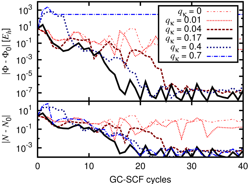
Figure 1: Dependence of GC-SCF convergence on low-frequency cutoff wavevector $q_{\kappa}$. The upper panel shows the convergence of the grand free energy $\Phi$ (towards its final value $\Phi_{0}$) on a logarithmic scale, and the lower panel shows that of the electron number $N$ (towards its final value $N_{0}$). Best convergence is obtained with $q_{\kappa}=0.17a_{0}^{-1}$, the inverse Debye-screening length, which we use as the default value henceforth. Results shown here are for a five-layer (5ML) Cu(111) slab solvated in 1M CANDLE aqueous electrolyte, with potential fixed to 1V SHE ($\mu=-0.208E_{h}$), starting from a converged neutral calculation of the same slab in vacuum.

The self-consistent field (GC-SCF) algorithm summarized in section II.1 depends on several parameters that control its iterative convergence. All these parameters are common to the conventional fixed-charge version (SCF) and the fixed-potential variant (GC-SCF) introduced here, except for the low-frequency cutoff wavevector $q_{\kappa}$ that is necessary to allow the net electron number to change in the fixed-potential case. Figure 1 compares the dependence of GC-SCF convergence on $q_{\kappa}$ for a prototypical calculation of an electrochemical system: a Cu(111) surface treated using a five-layer inversion-symmetric slab surrounded by 1M aqueous non-adsorbing electrolyte treated using the CANDLE solvation model,Sundararaman and Goddard III (2015) at a fixed potential of $\mu=-0.208E_{h}$ (1V SHE). (The remaining GC-SCF parameters are set to their default values which we discuss below.) The best convergence is obtained with $q_{\kappa}=0.17$ which corresponds to the Debye screening length of the electrolyte (21). For small $q_{\kappa}$, including the conventional case of $q_{\kappa}=0$, the number of electrons does not respond sufficiently quickly, stalling at about 0.1 electrons from the converged value, correspondingly with the free energy stalling at about 0.1 $E_{h}$ ($\approx 2.7$ eV) away from the converged value. Larger $q_{\kappa}$ causes the electron number to change too rapidly, hindering convergence and eventually leading to a divergence as seen for the case of $q_{\kappa}=0.7$. An issue remains in the convergence independent of $q_{\kappa}$: after initial convergence, the free energy oscillates at the $10^{-6}~{}E_{h}$ level, while the electron number oscillates at the $10^{-3}$ level.

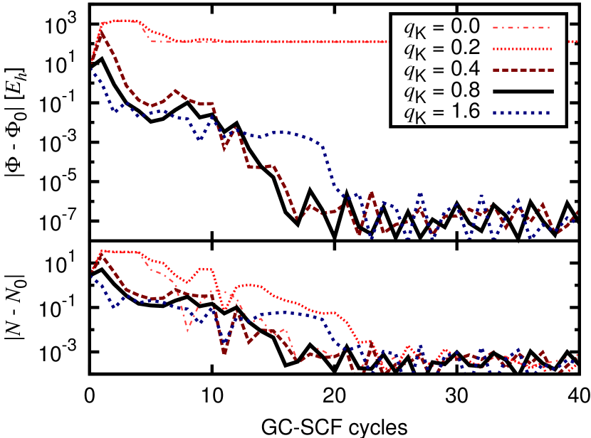
Figure 2: Dependence of GC-SCF convergence on Kerker-mixing wavevector $q_{K}$. Good convergence is observed near the typical recommended value $q_{K}=0.8~{}a_{0}^{-1}$ ($\approx 1.5$ Å${}^{\textrm{-1}}$). Convergence is relatively insensitive to $q_{K}$ near this value, but becomes unstable for small $q_{K}$ approaching the low-frequency cutoff $q_{\kappa}$. System and remaining details are identical to Figure 1.

Keeping $q_{\kappa}$ at this optimum value given by (21), we next examine the dependence of GC-SCF convergence on the remaining algorithm parameters for the same example system. Figure 2 shows the dependence on the Kerker mixing wavevector $q_{K}$, which helps stabilize the GC-SCF algorithm against long-wavelength charge oscillations. Optimal convergence is obtained for the typical recommended valueKresse and Furthmüller (1996) of $0.8~{}a_{0}^{-1}$ ($\approx 1.5$ Å${}^{\textrm{-1}}$). As expected, convergence is relatively insensitive to the exact choice of $q_{K}$, as long as $q_{K}$ does not become so small that convergence is ruined by charge sloshing. Notice that the final convergence beyond the $10^{-6}~{}E_{h}$ and $10^{-3}$ electron level remains an issue that is not resolved for any choice of $q_{K}$.

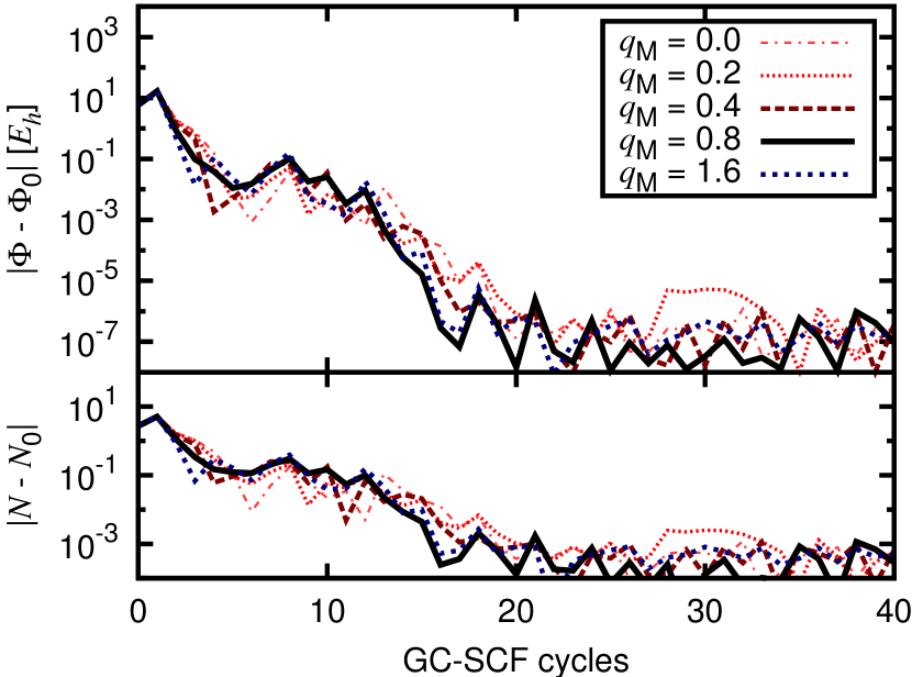
Figure 3: Dependence of GC-SCF convergence on Pulay-metric wavevector $q_{M}$. Convergence is relatively insensitive to $q_{M}$, and we set $q_{M}=q_{K}=0.8~{}a_{0}^{-1}$ henceforth. System and remaining details are identical to Figure 1.

Next, Figure 3 shows the variation of GC-SCF convergence with the wavevector $q_{M}$ controlling the reciprocal-space metric used by the Pulay algorithm. The convergence is entirely insensitive to this choice, and we henceforth set $q_{M}=q_{K}=0.8~{}a_{0}^{-1}$ (the recommended valueKresse and Furthmüller (1996)). Again, the final convergence issue remains unaffected by the choice of $q_{M}$.

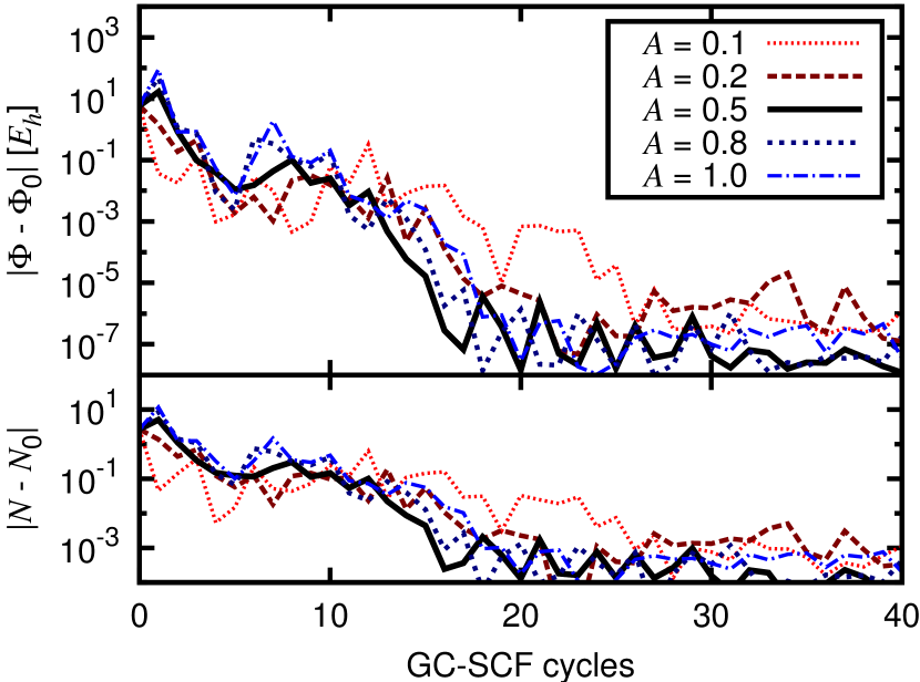
Figure 4: Dependence of GC-SCF convergence on maximum Kerker-mixing fraction $A$. Convergence is relatively insensitive to $A$, except that it slows down for small $A$ We henceforth set $A=0.5$ which nominally exhibits the best convergence. System and remaining details are identical to Figure 1.

Finally, Figure 4 compares the dependence of GC-SCF convergence on the maximum Kerker mixing fraction $A$, which effectively controls what fraction of the new electron density is mixed into the current value. We find nominally best convergence for $A=0.5$, but the performance of other values is not much worse. Smaller values of $A$ lead to greater stability initially, but marginally slower convergence later on, while larger values of $A$ lead to greater oscillations initially, but faster convergence later on. Regardless, as before, good convergence is obtained until the free energy reaches the $10^{-6}~{}E_{h}$ level, but continues to oscillate at that level beyond that point.

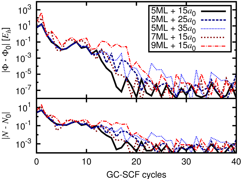
Figure 5: Variation of GC-SCF convergence using the default parameters determined above with system size: both with number of slab layers ranging from 5ML to 9ML with fixed vacuum spacing 15 $a_{0}$, and with vacuum spacing ranging from 15 $a_{0}$ to 35 $a_{0}$ with the 5ML slab. Convergence slows only marginally with increasing system size, with either vacuum spacing or layer count. Each calculations is for solvated Cu(111) charged to 1V SHE in CANDLE electrolyte, starting from the state of the corresponding converged neutral vacuum calculation.

This final convergence issue may not affect practical calculations where relevant energy differences are at the $10^{-}3~{}E_{h}$ level or higher. However, smooth exponential convergence to the final answer is desirable as this makes it easier to determine when the target accuracy has been reached. Unfortunately, no combination of GC-SCF parameters achieves uniformly smooth convergence for the fixed-potential case. On the other hand, with our $q_{\kappa}$ modification, the GC-SCF algorithm at least converges to the $10^{-6}~{}E_{h}$ level independent of system size (Figure 5), with the number of cycles required for convergence remaining mostly unchanged with increasing number of Cu(111) layers, and with increasing thickness of the solvent region.

Note that the standard fixed-charge SCF method converges the energy smoothly and exponentially in most cases, including in our implementation in JDFTx. Our implementation of the GC-SCF method in JDFTx uses exactly the same code, except for the preconditioner and metric modifications (due to $q_{\kappa}$) presented here. Therefore we believe that the final convergence difficulty in GC-SCF is a property of the algorithm itself, rather than an implementation issue.

III.3 Convergence of the GC-AuxH method

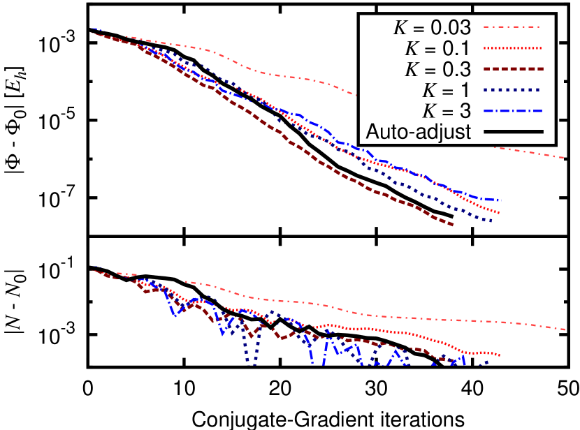
Figure 6: Dependence of the convergence of the GC-AuxH variational-minimize method on $K$, the preconditioning scale factor for subspace rotations generated by the auxiliary Hamiltonian. Near-optimal convergence is obtained when $K$ is automatically adjusted using the heuristic given by (29), which we use by default henceforth. Calculations are for solvated 5ML Cu(111) at 1V SHE, starting from the corresponding neutral vacuum calculation, exactly as in Figures 1-4. Note the smooth exponential convergence (without oscillations in electron number and free energy) here, in contrast to the GC-SCF case.

The grand-canonical auxiliary Hamiltonian (GC-AuxH) approach discussed in section II.2, directly minimizes the total free energy of the system without assuming any models for physical properties of the system (such as dielectric response models that are built into the SCF mixing schemes). This algorithm contains a single parameter $K$, which weights the relative contributions of the Kohn-Sham orbital and subspace Hamiltonian degrees of freedom in the conjugate-gradients search direction for free energy minimization.

Figure 6 shows the dependence of iterative convergence of the GC-AuxH algorithm on this preconditioning parameter $K$ for the same Cu(111) test problem considered above. If the preconditioning factor $K$ is held fixed, the rate of convergence is sensitive to the choice of $K$, with the optimum choice being $K\approx 0.3$ for this system. With the preconditioner auto-adjusted using the heuristic given by (29), we find that indeed the convergence picks up from that of the sub-optimal $K=1$ towards that of the optimal value. More importantly, we observe smooth exponential convergence of both the free energy and the electron number, in contrast to our experiences with the GC-SCF method.

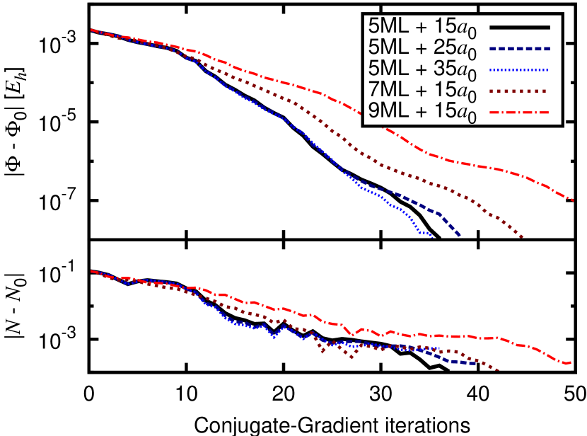
Figure 7: Variation of convergence of the GC-AuxH variational-minimize method with Cu(111) system size (exactly analogous to Figure 5 for the GC-SCF method). Convergence is invariant with vacuum spacing, and slows down only marginally with number of layers.

Figure 7 further shows that this smooth convergence sustains with changing system size. In particular, the convergence is virtually unchanged with the thickness of the solvent regions, but slows down slightly with increasing number of copper layers in the surface slabs.

III.4 Comparison of algorithms

Having analyzed and optimized the convergence of the GC-SCF and GC-AuxH methods, we now compare the performance of these algorithms for a few different cases. In this comparison, we also include the present state of the art: the ‘Loop’ method which uses a secant method to adjust the number of electrons in an outer loop to match the specified electron chemical potential.Goodpaster, Bell, and Head-Gordon (2016) For a fair comparison, we use the fixed-charge SCF method in the inner loops, because it achieves the fastest convergence; this algorithm works equally well with the AuxH method in the inner loop, but is then marginally slower. In each test case, we start all three algorithms from the same starting point: the converged state of the corresponding neutral (fixed-charge) calculation. Different test cases effectively perturb the potential by different amounts, thereby testing the algorithms for a range of proximities between initial and final states. Also, we now compare the wall time between algorithms, because there is no straightforward correspondence between GC-SCF cycles and conjugate-gradient iterations of the GC-AuxH method. The relative wall-time performance of these fairly distinct algorithms will depend to an extent on details of code optimization for each. However, there is no perfect metric for comparing these algorithms and wall time suffices for a rough qualitative comparison.

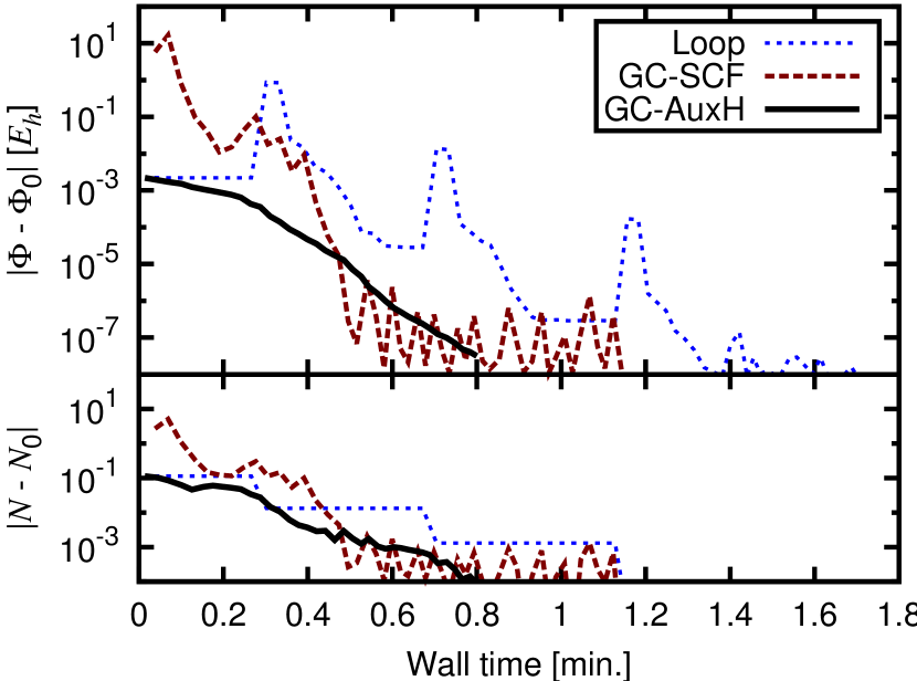
Figure 8: Performance comparison of the new GC-SCF and GC-AuxH methods with the previous state of the art: a ‘Loop’ over fixed-charge calculations (using the secant method to adjust the charge to match the potential). Both new methods reach $10^{-7}~{}E_{h}$ free energy accuracy in half the wall time of the Loop method, but the GC-AuxH method is the clear winner with smooth exponential convergence. Calculations here are for the 5ML Cu(111) slab at 1V SHE, as before. Timings are measured on a single 32-core NERSC Cori node in all cases.

First, Figure 8 compares the performance of the algorithms for the 5-layer Cu(111) slab used in all the tests so far. The spikes in the free energy seen in the Loop method are the points where the electron number changes in the outer loop and a new SCF convergence at fixed charge begins. Both the GC-SCF and GC-AuxH methods are quite competitive, cutting the time to convergence within $10^{-6}~{}E_{h}$ in half compared to the Loop method. Given the smooth convergence beyond $10^{-6}~{}E_{h}$ however, the GC-AuxH method is preferable over GC-SCF for fixed potential calculations. Note that in the fixed-charge case, when SCF converges smoothly, it often outperforms the AuxH method as mentioned above. The advantage of the AuxH and GC-AuxH method is their stability on account of being variational methods: the free energy is guaranteed to decrease at every step. Consequently, the convergence difficulties of the GC-SCF method make the variationally stable GC-AuxH method relatively more attractive.

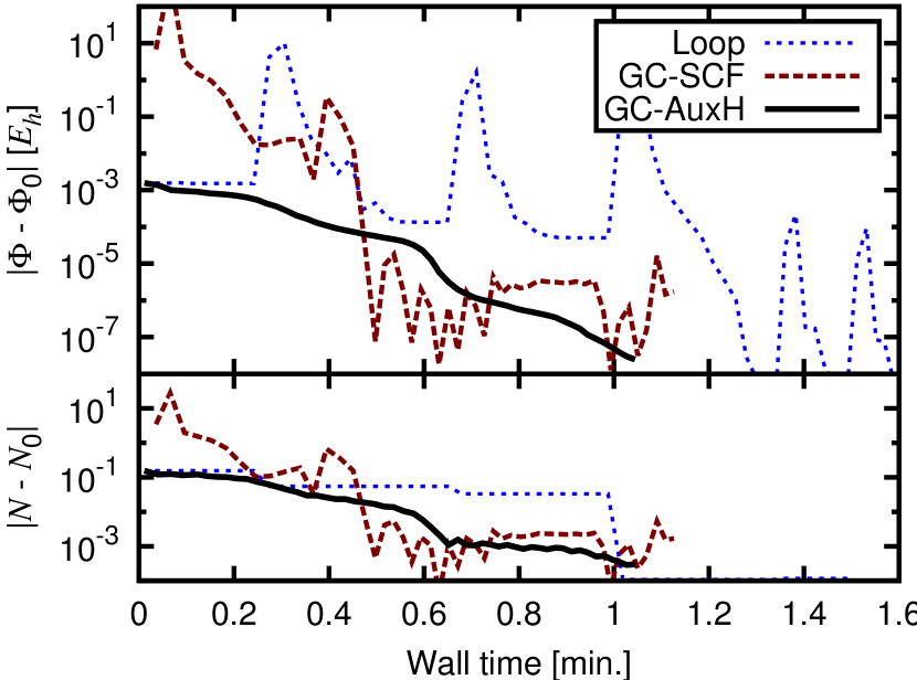
Figure 9: Similar to Figure 8, but for a 5ML Pt(111) slab at 0V SHE ($\mu=-0.171~{}E_{h}$). Platinum is neutral at $\approx 0.8$V SHE, so this corresponds to negatively charging the slab, which activates CANDLE’s asymmetry correction. Additionally, platinum has $d$ bands crossing the Fermi level in contrast to copper which has occupied $d$ bands. This calculation therefore explores a more complicated charge vs. potential landscape, causing deviations from exponential convergence, but the relative performance of the algorithms remains similar.

Next, we compare these algorithms for more complex text cases. Figure 9 compares the convergence for a five-layer Pt(111) slab fixed to a potential of $\mu=-0.171~{}E_{h}$ (0V  SHE). At this potential, the surface of Pt(111) charges negatively, and the CANDLE solvation model brings the cavity closer to the electrons to capture the more effective solvation of negative charges by liquid water. Additionally, the dielectric response of platinum is more complex than copper due to the partially filled $d$ shell. Both of these factors make this system harder to converge than the previous test case, and therefore the convergence of the GC-AuxH method is no longer clearly a single exponential. Despite this, both the direct grand-canonical methods converge faster than the Loop method, with the GC-AuxH method eking out an advantage in final convergence as before.

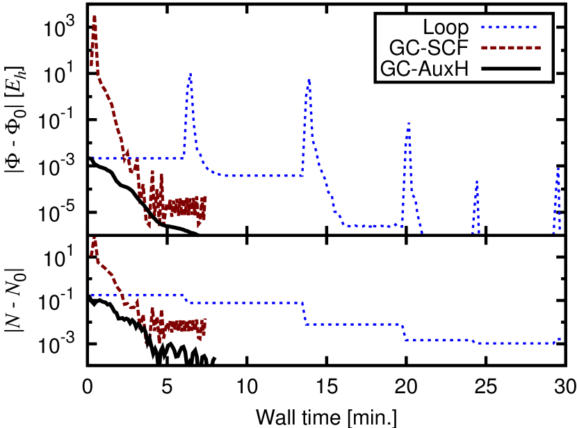
Figure 10: Similar to Figures 8 and 9, but for a 5ML Pt(111) slab decorated with a $\sqrt{3}\times\sqrt{3}$ partial monolayer of adsorbed chloride anions (1/3 coverage) at 0V SHE. The increased complexity slows down the convergence of the GC-SCF method, which also slows down the Loop over fixed-charge SCF calculations, while the GC-AuxH method continues to exhibit rapid near-exponential convergence with no charge oscillations, beating the Loop method by a factor of 4 in time. All subsequent calculations of complex metal surfaces with adsorbates therefore use the GC-AuxH method.

Finally, Figure 10 compares the convergence for chloride anions adsorbed at one-third monolayer coverage, in a $\sqrt{3}\times\sqrt{3}$ supercell of a five-layer Pt(111) slab. Despite the increased complexity, the direct grand-canonical methods exhibit the best convergence, edging out the Loop method by a factor of four in wall time now, again with smoothest convergence for the GC-AuxH method. Due to the systematic convergence advantage of the GC-AuxH method, we use it for all remaining calculations in this work and recommend it as the default general purpose algorithm for converging electrochemical calculations.

In the theory section and all calculations so far, we used Fermi smearing where the electron occupations are given by the Fermi function (6). Practical $k$-point meshes typically require the use of a temperature $T$ substantially higher than room temperature (we used 0.01 $E_{h}$ which is approximately ten times higher), which could result in inaccurate free energies. Such errors can be reduced substantially by changing the functional form of the occupations and the electronic entropy, with the caveat that the smearing width $T$ no longer corresponds to an electron temperature. Common modifications include Gaussian smearing, where the Fermi functions are replaced with error functions, and Cold smearing,Marzari et al. (1999) where the functional form is chosen to cancel the lowest order variation of the free energy with $T$. (See Ref. 45 for details.)

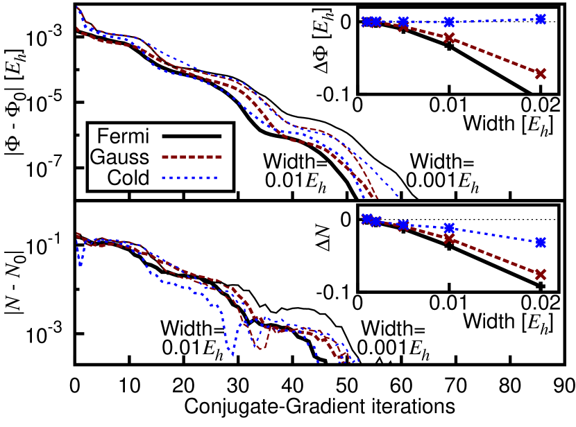
Figure 11: Comparison of the convergence of the GC-AuxH method for the 5ML Pt(111) slab at 0V SHE using different smearing functions. Insets show the variation of converged properties with smearing width. Cold smearingMarzari et al. (1999) substantially reduces the finite-width error in the free energy, and to a lesser extent in the electron number, compared to Gaussian and Fermi smearing. At the same width of 0.01 $E_{h}$, the GC-AuxH method with cold smearing converges marginally slower than Gaussian or Fermi smearing, but still faster than when using any of the smearing methods with the smaller width of 0.001 $E_{h}$.

Figure 11 compares the performance of the preferred GC-AuxH method for various smearing methods. The insets show the variation of the converged free energy and electron number with smearing width $T$. Gaussian smearing reduces the coefficient of the quadratic $T$ dependence compared to Fermi smearing, while Cold smearing cancels the quadratic dependence altogether, by design. The variation of electron number with smearing width is also reduced by Cold smearing, but to a lesser extent. Notice that the use of Cold smearing marginally slows down the iterative convergence of the GC-AuxH method. However, using Cold smearing at a high width of 0.01 $E_{h}$ is still faster than using any smearing method with the lower width 0.001 $E_{h}$ that is close to room temperature (because of the far denser Brillouin zone sampling required for smaller widths). Therefore, it is still advantageous to use Cold smearing at elevated smearing widths, and so we use Cold smearing with a width of 0.01 $E_{h}$ for the final demonstration below.

III.5 Under-potential deposition of Cu on Pt(111)

The application of sufficiently negative (reductive) potentials on an electrode immersed in a solution containing metal ions, reduces those ions and results in bulk electro-deposition of metal on the surface. Additionally, for many pairs of metals, a single monolayer of one metal deposits on a surface of the other at an under potential, that is, at a potential less favorable than for bulk deposition. This phenomenon of under-potential deposition (UPD) has several technological applications since it enables precise synthesis of heterogeneous metal interfaces. It also serves as an archetype for fundamental studies of electrochemical processes (see Ref. 46 for an extensive review), which makes it a perfect example for demonstrating our grand-canonical density-functional theory method.

The basic reason for underpotential deposition is that the heterogeneous binding between the two metals is stronger than the homogeneous binding of the depositing metal to itself. Indeed, metal pairs that exhibit underpotential deposition also display analogous phenomena in vapor adsorption.Paffett et al. (1985). However, the process in solution is far more complicated and highly sensitive to the composition of the solution because of competing adsorbates,White and Abruña (1991) as well as to the structure of the electrode surface.Abruña et al. (1998)

The UPD of copper on Pt(111) in the presence of chloride anions is particularly interesting and the subject of considerable debate in the literature. Voltammetry for this systemBludau et al. (1998) exhibits two well-separated under-potential peaks, as shown in the background of Figure 12. Certain LEED and in situ X-ray scattering studies of this systemMarkovic et al. (1995) find evidence of a $2\times 2$ bilayer of copper and chloride ions co-adsorbed on the surface at potentials between the two peaks, suggesting that one peak corresponds to a formation of a partial layer, and the second peak, to the formation of the full monolayer. In contrast, other studiesSoldo et al. (2002); Bludau et al. (1998); amd K. Wu, Eiswirth, and Ertl (1999) do not find this signature and propose that the additional peak arises from adsorption and desorption of chloride ions alone.

To address this debate, we perform grand-canonical density functional theory calculations of various configurations of copper and chlorine adsorbed on a 5-layer Pt(111) slab in $\sqrt{3}\times\sqrt{3}$ and $2\times 2$ supercells. We determine the most stable configurations at each potential($\mu$) and the potentials at which transitions between configurations occur by comparing their grand free energies. The relevant grand free energy of a configuration $\alpha$ containing $N_{\textrm{Pt}}^{\alpha}$ platinum atoms in the slab with $N_{\textrm{Cu}}^{\alpha}$ copper and $N_{\textrm{Cl}}^{\alpha}$ chlorine atoms adsorbed at the surface within the calculation cell is

$$\tilde{\Phi}^{\alpha}(\mu)=\frac{\Phi^{\alpha}(\mu)-\mu_{\textrm{Pt}}N_{\textrm{Pt}}^{\alpha}-\mu_{\textrm{Cu}}N_{\textrm{Cu}}^{\alpha}-\mu_{\textrm{Cl}}N_{\textrm{Cl}}^{\alpha}}{N_{\textrm{Pt}}^{\textrm{surf}}},$$ (30)

normalized by the number of surface platinum atoms $N_{\textrm{Pt}}^{\textrm{surf}}$ in order to correctly compare energies of calculations in different supercells. ($N_{\textrm{Pt}}^{\textrm{surf}}=2$ for the unit cell, 6 for the $\sqrt{3}\times\sqrt{3}$ supercell and 8 for the $2\times 2$ supercell, accounting for the top and bottom surfaces in the inversion-symmetric setup.) Since no light atoms are present, we safely neglect changes in vibrational contributions to the free energy between adsorbate configurations.

Above, $\Phi^{\alpha}(\mu)$ is the free energy of adsorbate configuration $\alpha$ calculated by fixed-potential DFT, which is grand canonical with respect to the electrons at chemical potential $\mu$ (related to the electrode potential by (14) as discussed at the end of Section I.2). Then, (30) above calculates the free energy $\tilde{\Phi}^{\alpha}(\mu)$ which is additionally grand canonical with respect to all relevant atoms with chemical potentials $\mu_{\textrm{Pt}}$, $\mu_{\textrm{Cu}}$ and $\mu_{\textrm{Cl}}$. Several conventions are possible in defining the electron-grand-canonical free energy $\Phi$, depending on what electron number we subtract: change from neutral value, total electron number, or number of valence electrons in pseudopotential DFT calculations. The atom chemical potentials would then respectively correspond to neutral atoms, bare nuclei or pseudo-nuclei (nuclei + core electrons in pseudopotential). The full grand canonical free energy $\tilde{\Phi}$ does not depend on this choice. In our JDFTx implementation, we choose the last option above (number of valence electrons and correspondingly atom chemical potentials of the pseudo-nuclei).

The bulk of the platinum electrode sets the Pt chemical potential, $\mu_{\textrm{Pt}}=E_{\textrm{Pt(s)}}-\mu N^{e}_{\textrm{Pt(s)}}$, where $E_{\textrm{Pt(s)}}$ is the DFT energy of a bulk fcc Pt calculation with a single atom in the unit cell, and $N^{e}_{\textrm{Pt(s)}}$ is the number of valence electrons in that calculation. The second term here implements the electron counting convention discussed above. Next, copper ions in solution set $\mu_{\textrm{Cu}}$, but directly calculating the free energy of such ions using solvation models is error-prone.Sundararaman and Goddard III (2015) So, instead, we use the DFT calculated energy, $E_{\textrm{Cu(s)}}$, of a bulk fcc Cu calculation (containing $N^{e}_{\textrm{Cu(s)}}$ valence electrons), and relate it to the free energy of the ion via the experimentally-determined standard reduction potential $U_{\textrm{Cu${}^{\textrm{2+}}$$\rightarrow$Cu(s)}}=0.342$ V SHE.Haynes (2012) This yields

$$\mu_{\textrm{Cu}}=\left(E_{\textrm{Cu(s)}}-\mu N^{e}_{\textrm{Cu(s)}}\right)\\ +2\left(\mu-\mu_{\textrm{SHE}}+eU_{\textrm{Cu${}^{\textrm{2+}}$$\rightarrow$Cu(s)}}\right)\\ +k_{B}T\ln[\mathrm{Cu}^{2+}],$$ (31)

where the second term accounts for the change from Cu(s) to $\mathrm{Cu}^{2+}$ ions, and the final term accounts for change in ionic concentration from the standard value of 1 mol/liter to the current value of [Cu²⁺] (in mol/liter). Similarly, chlorine ions in solution set $\mu_{\textrm{Cl}}$, but to minimize DFT errors, we connect to the DFT calculated energy, $E_{\textrm{Cl(at)}}$, of an isolated Chlorine atom (containing $N^{e}_{\textrm{Cl(at)}}$ valence electrons), via the experimentally-determined atomization energy $E_{\textrm{Cl${}_{\textrm{2}}$$\rightarrow$2Cl(at)}}=242.6$ kJ/mol,ccc gas-phase entropy $S_{\textrm{Cl${}_{\textrm{2}}$(g)}}=223.1$ J/mol-K,Haynes (2012) and reduction potential $U_{\textrm{Cl${}_{\textrm{2}}$(g)$\rightarrow$2Cl${}^{-}$}}=1.358$ V SHE.Haynes (2012) Specifically,

$$\mu_{\textrm{Cl}}=\left(E_{\textrm{Cl(at)}}-\mu N^{e}_{\textrm{Cl(at)}}\right)-\frac{1}{2}\left(E_{\textrm{Cl${}_{\textrm{2}}$$\rightarrow$2Cl(at)}}+TS_{\textrm{Cl${}_{\textrm{2}}$(g)}}\right)\\ -\left(\mu-\mu_{\textrm{SHE}}+eU_{\textrm{Cl${}_{\textrm{2}}$(g)$\rightarrow$2Cl${}^{-}$}}\right)\\ +k_{B}T\ln[\mathrm{Cl}^{-}],$$ (32)

where the second term accounts for the change from atomic to gas-phase chlorine, the third term for the change to chloride ions, and the final term for the change in chloride ion concentration to [Cl^-] (in mol/liter).

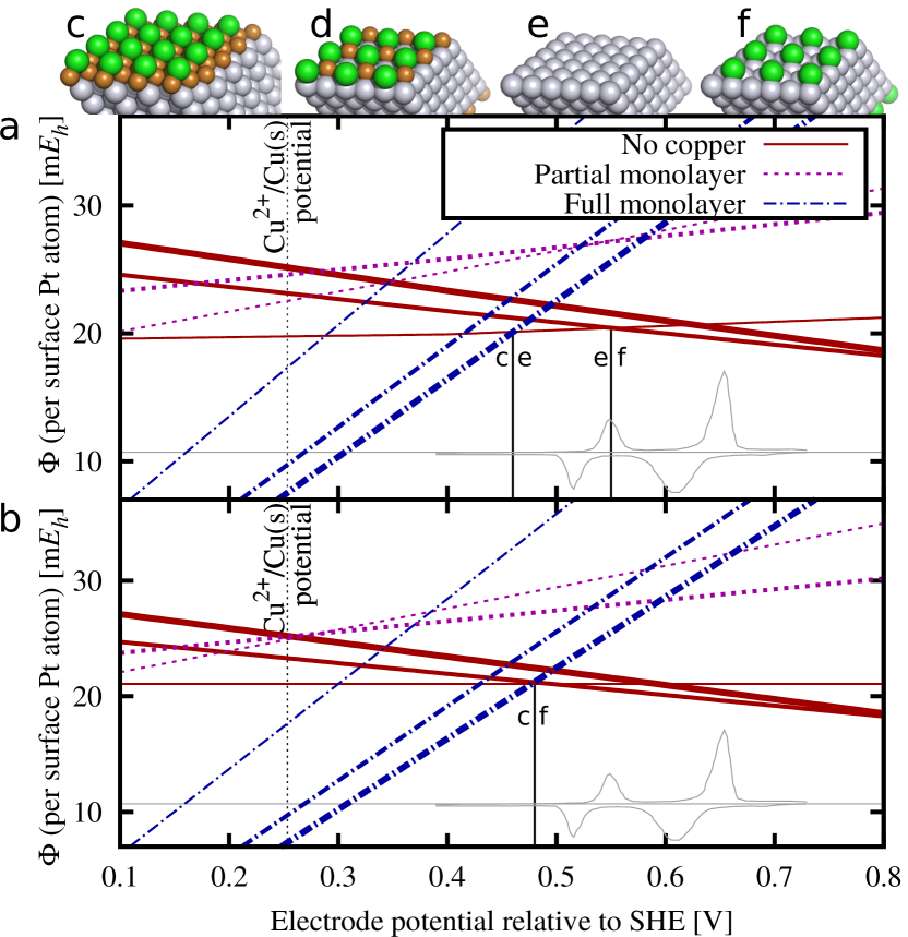
Figure 12: Underpotential deposition of Cu on Pt(111) from an aqueous solution containing 10^-3 mol/liter Cu${}^{\textrm{2+}}$ ions and 10^-4 mol/liter Cl^- ions. Calculated free energies for various adsorbate configurations as a function of electrode potential are shown as calculated by explicit fixed-potential solvated calculations in (a), and from vacuum calculations in (b), with the experimental voltammogramBludau et al. (1998) shown for comparison. Solid red lines indicate no copper, purple dotted lines indicate $2\times 2$ partial copper monolayer and blue dot-dash lines indicate full copper monolayer. Thickness of the lines indicate Cl coverage, ranging from no Cl (thinnest), $2\times 2$ (1/4) coverage (intermediate) to $\sqrt{3}\times\sqrt{3}$ (1/3) coverage (thickest). Prominent configurations are sketched in (c-f). Vacuum calculations in (b) predict only a single voltammetric peak in disagreement with experiment. Explicit potential-dependent solvated calculations in (a) predict two peaks in qualitative agreement with experiment ($\sim 0.1$ V accuracy), with the second peak due to chloride desorption.Soldo et al. (2002); Bludau et al. (1998); amd K. Wu, Eiswirth, and Ertl (1999) The partial Cu monolayer (d) proposed by someMarkovic et al. (1995) is not predicted to be the most stable configuration at any relevant potential.

Figure 12(a) shows the calculated grand free energies as a function of electrode potential for a number of Cu and Cl adsorbate configurations on the surface of Pt(111). At high potentials, the most stable (lowest free energy) configuration is 1/4 Cl coverage (Figure 12(f)), which transitions to a clean Pt surface (Figure 12(e)) at a potential of 0.55 V SHE. Upon further lowering the potential, the stable configuration transitions to a full monolayer of copper with 1/3 Cl coverage (Figure 12(c)) at a potential of 0.46 V SHE. Experimentally, the two voltammogram peaks are at approximately $(0.63\pm 0.04)$ and $(0.51\pm 0.02)$ V SHE, averaging over the forward and reverse direction sweeps. Therefore chlorine desorption and full-copper-monolayer formation are plausible explanationsSoldo et al. (2002); Bludau et al. (1998); amd K. Wu, Eiswirth, and Ertl (1999) of the two peaks, with our first-principles predictions reproducing well the peak spacing (0.09 eV versus 0.12 eV in experiment), and placing the absolute locations of the peaks to within 0.07 eV. Similar accuracy has been achieved in comparison to experiment for onset potentials and product selectivity in CO reduction on Cu(111)Xiao et al. (2016); Xiao, Cheng, and Goddard III (2017) and the oxygen evolution reaction on IrO2(110)Ping, Nielsen, and Goddard III (2017) in concurrent work using exactly the same calculation protocol as here: fixed-potential DFT in JDFTx using the PBE exchange-correlation functional and the CANDLE solvation model. The partial 2x2 monolayer of copper (Figure 12(d)) proposed by othersMarkovic et al. (1995) as the reason for the second peak is not the most stable configuration in our calculations at any potential, lying a significant 0.3 eV above the other phases at relevant potentials.

For comparison, Figure 12(b) shows the analogous results that would be obtained using only conventional vacuum calculations. In the above formalism, this corresponds to assuming $\Phi^{\alpha}(\mu)\approx A^{\alpha}-\mu N_{e}^{\alpha}$, where $A^{\alpha}$ is the Helmholtz energy from a neutral vacuum DFT calculation of configuration $\alpha$ containing $N_{e}^{\alpha}$ valence electrons. This approximation results in a single transition directly from the Cl-covered Pt surface to the one with a copper monolayer, predicting a single voltammogram peak in disagreement with experiment. Accurate predictions for electrochemical systems therefore require treating charged configurations stabilized by the electrolyte at relevant electron potentials, now easily accomplished with the methods and algorithms introduced in this work.

Conclusions

This work introduces algorithms for directly converging DFT calculations in the grand-canonical ensemble of electrons, where the number of electrons adjusts to maintain the system at constant electron chemical potential, while ionic response in a continuum solvation model of electrolyte keeps the system neutral . We show that, with appropriate modifications, grand canonical versions of both the self-consistent field (GC-SCF) method as well as direct free-energy minimization with auxiliary Hamiltonians (GC-AuxH) method are able to rapidly converge the grand free energy of electrons. This substantially improves upon the current state of the art of running an outer loop over conventional fixed-charge DFT calculations. With detailed tests of the convergence of all these algorithms, we show that the GC-AuxH method is the most suitable default choice exhibiting smooth exponential convergence to the minimum.

Grand-canonical DFT directly mimics the experimental condition in electrochemical systems, where electrode potential sets the chemical potential of electrons, and the number of electrons at the electrode surface (including adsorbates in the electrochemical interface) changes continuously in response. Describing this change in charge at the surface plays an important role in accurately modeling several electrochemical phenomena.Schwarz et al. (2015, 2016); Xiao et al. (2016); Goodpaster, Bell, and Head-Gordon (2016) Here, we showcase the new algorithms by analyzing the under-potential deposition (UPD) of copper on platinum in an electrolyte containing chloride ions. We resolve an old debate about the identity of a second under-potential peak, showing that partial copper monolayers are not plausible and that the second peak is due to desorption of chloride ions. We expect the new methods presented here to substantially advance the realistic treatment of electrochemical phenomena in first principles calculations.