Asymptotic behaviour of ground states for mixtures
of ferromagnetic and antiferromagnetic interactions
in a dilute regime

Abstract

We consider randomly distributed mixtures of bonds of ferromagnetic and antiferromagnetic type in a two-dimensional square lattice with probability $1-p$ and $p$, respectively, according to an i.i.d. random variable. We study minimizers of the corresponding nearest-neighbour spin energy on large domains in $\mathbb{Z}^{2}$. We prove that there exists $p_{0}$ such that for $p\leq p_{0}$ such minimizers are characterized by a majority phase; i.e., they take identically the value $1$ or $-1$ except for small disconnected sets. A deterministic analogue is also proved.

1 Introduction

We consider randomly distributed mixtures of bonds of ferromagnetic and antiferromagnetic type in a two-dimensional square lattice with probability $1-p$ and $p$, respectively, according to an i.i.d. random variable. For each realization $\omega$ of that random variable, we consider, for each bounded region $D$, the energy

$$F^{\omega}(u,D)=-\sum_{i,j}c^{\omega}_{ij}u_{i}u_{j},$$

where the sum runs over nearest-neighbours in the square lattice contained in $D$, $u_{i}\in\{-1,+1\}$ is a spin variable, and $c^{\omega}_{ij}\in\{-1,+1\}$ are interaction coefficients corresponding to the realization.

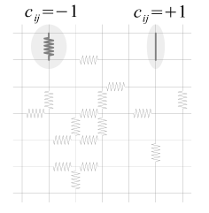
Figure 1: representation of a portion of spin system for some $c_{ij}=c^{\omega}_{ij}$

A portion of such a system is pictured in Fig. 1: ferromagnetic bonds; i.e, when $c^{\omega}_{ij}=1$, are pictured as straight segments, while antiferromagnetic bonds are pictured as wiggly ones (as in the two examples highlighted by the gray regions, respectively).

In this paper we analyze ground states; i.e., absolute minimizers, for such energies. This is a non trivial issue since in general, ground states $\{u_{j}\}$ are frustrated; i.e., the energy cannot be separately minimized on all pairs of nearest neighbors. In other words, minimizing arrays $\{u_{j}\}$ may not satisfy simultaneously $u_{i}=u_{j}$ for all $i,j$ such that $c^{\omega}_{ij}=+1$ and $u_{i}=-u_{j}$ for all $i,j$ such that $c^{\omega}_{ij}=-1$. However, in [14] it is shown that if the antiferromagnetic links are contained in well-separated compact regions, then the ground states are characterized by a “majority phase”; i.e., they mostly take only the value $1$ (or $-1$) except for nodes close to the “antiferromagnetic islands”. In the case of random interactions we show that this is the same in the dilute case; i.e., when the probability $p$ of antiferromagnetic interactions is sufficiently small. More precisely, we show that there exists $p_{0}$ such that if $p$ is not greater than $p_{0}$ then almost surely for all sufficiently large regular bounded domain $D\subset{\mathbb{R}}^{2}$ the minimizers of the energy $F(\cdot,D)$ are characterized by a majority phase.

The proof of our result relies on a scaling argument as follows: we remark that proving the existence of majority phases is equivalent to ruling out the possibility of large interfaces separating zones where a ground state $u$ equals $1$ and $-1$, respectively. Such interfaces may exist only if the percentage of antiferromagnetic bonds on the interface is larger than $1/2$. We then estimate the probability of such an interface with a fixed length and decompose a separating interface into portions of at most that length, to prove a contradiction if $p$ is small enough.

Interestingly, the probabilistic proof outlined above carries on also to a deterministic periodic setting; i.e., for energies

$$F(u,D)=-\sum_{i,j}c_{ij}u_{i}u_{j}$$

such that $c_{ij}\in\{-1,+1\}$ and there exists $N\in\mathbb{N}$ such that $c_{i+k\,j+k}=c_{ij}$ for all $i$ and $j\in\mathbb{Z}^{2}$ and $k\in N{\mathbb{Z}}^{2}$. In this case ground states of $F$ may sometimes be characterized more explicitly and exhibit various types of configurations independently of the percentage of antiferromagnetic bonds: up to boundary effects, there can be a finite number of periodic textures, or configurations characterized by layers of periodic patterns in one direction, or we might have arbitrary configurations of minimizers with no periodicity (see the examples in [9]). We show that there exists $p_{0}$ such that if the percentage $p$ of antiferromagnetic interactions is not greater than $p_{0}$ then the proportion of $N$-periodic systems $\{c_{ij}\}$ such that the minimizers of the energy $F(\cdot,D)$ are characterized by a majority phase for all $D\subset{\mathbb{R}}^{2}$ bounded domain large enough tends to $1$ as $N$ tends to $+\infty$. The probabilistic arguments are substituted by a combinatorial computation, which also allows a description of the size of the separating interfaces in terms of $N$.

This work is part of a general analysis of variational problems in lattice systems (see [7] for an overview), most results dealing with spin systems focus on ferromagnetic Ising systems at zero temperature, both on a static framework (see [18, 2, 8]) and a dynamic framework (see [11, 15, 16, 17]). In that context, random distributions of bonds have been considered in [14, 13] (see also [12]), and their analysis is linked to some recent advances in Percolation Theory (see [4, 19, 20, 22, 24]). A first paper dealing with antiferromagnetic interactions is [1], where non-trivial oscillating ground states are observed and the corresponding surface tensions are computed. A related variational motion of crystalline mean-curvature type has been recently described in [10], highlighting new effect due to surface microstructure. The classification of periodic systems mixing ferromagnetic and antiferromagnetic interactions that can be described by surface energies is the subject of [9]. In [14], as mentioned above, the case of well-separated antiferromagnetic island is studied. We note that in those papers the analysis is performed by a description of a macroscopic surface tension, which provides the energy density of a continuous surface energy obtained as a discrete-to-continuum $\Gamma$-limit [6] obtained by scaling the energy $F$ on lattices with vanishing lattice space. In the present paper we do not address the formulation in terms of the $\Gamma$-limit but only study ground states.

2 Random media

Given a probability space $(\Omega,\mathcal{F},\mathbf{P})$ we consider a Bernoulli bond percolation model in $\mathbb{Z}^{2}$. This means that to each bond $(i,j)$, $i,j\in\mathbb{Z}^{2}$, $|i-j|=1$, in $\mathbb{Z}^{2}$ we associate a random variable $c_{ij}$ and assume that these random variables are i.i.d. and that they take on the value $+1$ with probability $1-p$, and the value $-1$ with probability $p$, where $0<p<1$. The detailed description of the Bernoulli bond percolation model can be found for instance in [23]

We denote by $\mathcal{N}$ the set of nearest neighbors

$$\mathcal{N}=\{\{i,j\}:i,j\in\mathbb{Z}^{2},\|i-j\|=1\}$$

and, for each $\{i,j\}$ in $\mathcal{N}$, $[i,j]$ will be the closed segment with endpoints $i$ and $j$.

Definition 1 (random stationary spin system).

A (ferromagnetic/antiferromagnetic) spin system is a realization of the random function $c(\{i,j\})=c_{ij}(\omega)\in\{\pm 1\}$ defined on $\mathcal{N}$. We will drop the dependence on $\omega$ and simply write $c_{ij}$. The pairs $\{i,j\}$ with $c_{ij}=+1$ are called ferromagnetic bonds, the pairs $\{i,j\}$ with $c_{ij}=-1$ are called antiferromagnetic bonds.

2.1 Estimates on separating paths

We say that a finite sequence $(i_{0},\ldots,i_{k})$ is a path in $\mathbb{Z}^{2}$ if $\{i_{s},i_{s+1}\}\in\mathcal{N}$ for any $s=0,\ldots,k-1$ and the segment $[i_{s},i_{s+1}]$ is different from the segment $[i_{t},i_{t+1}]$ for any $s\neq t$. The path is closed if $i_{0}=i_{k}$. The number $k$ is the length of $\gamma$, denoted by $l(\gamma)$, and we call $\mathcal{P}_{k}$ the set of the paths with length $k$. To each path $\gamma\in\mathcal{P}_{k}$ we associate the corresponding curve $\tilde{\gamma}$ of length $k$ in $\mathbb{R}^{2}$ given by

$$\tilde{\gamma}=\bigcup_{s=0}^{k-1}[i_{s},i_{s+1}]+\Big{(}\frac{1}{2},\frac{1}{2}\Big{)}.$$ (1)

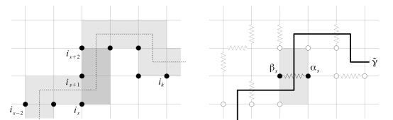
Figure 2: a path $\gamma$ and the corresponding curve $\tilde{\gamma}$

Note that $\tilde{\gamma}$ is a closed curve if and only if $\gamma$ is closed. In Fig. 2 we picture a path (the dotted sites of the left-hand side) and the corresponding curve (on the right-hand side picture).

Given two paths $\gamma=(i_{0},\dots,i_{k})$ and $\delta=(j_{0},\dots,j_{h})$, if $i_{k}=j_{0}$ and the sequence $(i_{0},\dots,i_{k},j_{1},\dots,j_{h})$ is a path, the latter is called the concatenation of $\gamma$ and $\delta$ and it is noted by $\gamma\ast\delta$.

We note that for each $s$ the intersection $(i_{s}+[0,1]^{2})\cap(i_{s+1}+[0,1]^{2})$ is a segment with endpoints $\{\alpha_{s},\beta_{s}\}\in\mathcal{N}$; then, given a spin system $\{c_{ij}\}$, for each path $\gamma=(i_{0},\ldots,i_{k})$ we can define the number of antiferromagnetic bonds of $\gamma$ as

$$\mu(\gamma)=\mu(\gamma,\{c_{ij}\})=\#\{s\in\{0,\dots,k-1\}:c_{\alpha_{s}\beta_{s}}=-1\}.$$ (2)

If $\tilde{\gamma}$ is the curve corresponding to $\gamma$ defined above, then the number $\mu(\gamma)$ counts the antiferromagnetic interactions “intersecting” $\tilde{\gamma}$ (see Fig. 2).

Definition 2 (Separating paths).

A path $\gamma$ of length $k$ is a separating path for a spin system $\{c_{ij}\}$ if $\mu(\gamma)>k/2$.

Remark 3.

The terminology separating path evokes the fact that only closed separating paths may enclose (separate) regions where a minimal $\{u_{i}\}$ is constant. Indeed, if we have $u_{i}=1$ on a finite set $A$ of nodes in $\mathbb{Z}^{2}$ which is connected (i.e., for every pair $i,j$ of points in $A$ there is a path of points in $A$ with $i$ as initial point and $j$ as final point) and $u_{i}=-1$ on all neighbouring nodes, then the boundary of $A$ (i.e., the set of points $i\in A$ with a nearest neighbour not in $A$) determines a path. If such a path is not separating then the function $\tilde{u}$ defined as $\tilde{u}_{i}=-u_{i}$ for $i\in A$ and $\tilde{u}_{i}=u_{i}$ elsewhere has an energy strictly lower than $u$.

Remark 4.

For a path $\gamma$ of length $l(\gamma)=k$ the probability that $\gamma$ be separating can be estimated as follows

$$\mathbf{P}\{\mu(\gamma)>k/2\}\leq p^{k/2}2^{k}$$ (3)

Indeed, the probability that $c_{ij}$ is equal to ${-1}$ at $k/2$ fixed places is equal to $p^{k/2}$. Since $\Big{(}\begin{array}[]{c}k\\ k/2\end{array}\Big{)}$ does not exceed $2^{k}$, the desired estimates follows.

Lemma 5.

There exists $p_{0}>0$ such that for any $\varkappa>0$ and for all $p<p_{0}$ almost surely for sufficiently large $n$ in a cube $Q_{n}=[0,n]^{2}$ there is no a separating path $\gamma$ with $l(\gamma)\geq(\log(n))^{1+\varkappa}$.

Proof.

We use the method that in percolation theory often called ”path counting”  argument. The number of paths of length $k$ starting at the origin is not greater than $3^{k}$. Therefore, in view of (3) the probability that there exists a separating path of length $k$ that starts at the origin is not greater than $p^{k/2}2^{k}3^{k}$. Letting $p_{0}=(1/12)^{2}$ we have

$$p^{k/2}2^{k}3^{k}\leq 2^{-k}\qquad\hbox{for all }p\leq p_{0}.$$

Then, if $p\leq p_{0}$, the probability that there exists a separating path of length $k$ in a cube $Q_{n}$ does not exceed $n^{2}2^{-k}$. For $k\geq\log(n)^{1+\varkappa}$ this yields

$$\mathbf{P}\{\hbox{there exists a separating path }\gamma\subset Q_{n}\hbox{ of length }k\}$$

$$\leq n^{2}2^{-\log(n)^{1+\varkappa}}=n^{2-c_{1}\log(n)^{\varkappa}}$$

with $c_{1}=\log 2$. Finally, summing up in $k$ over the interval $[\log(n)^{1+\varkappa},n^{2}]$ we obtain

$$\mathbf{P}\{\hbox{there exists a separating path }\gamma\subset Q_{n}\hbox{ such that }l(\gamma)\geq\log(n)^{1+\varkappa}\}$$

$$\leq n^{4-c_{1}\log(n)^{\varkappa}}$$

Since for large $n$ the right-hand side here decays faster than any negative power of $n$, the desired statement follows from the Borel-Cantelli lemma. ∎

2.2 Geometry of minimizers in the random case

Let $D$ be a bounded open subset of $\mathbb{R}^{2}$ and $u\colon D\cap\mathbb{Z}^{2}\to\{\pm 1\}$. Then, denoting by $\mathcal{N}(D)$ the set of nearest neighbors in $D$, $F(u,D)$ is defined by

$$F(u,D)=-\sum_{\{i,j\}\in\mathcal{N}(D)}c_{ij}u_{i}u_{j}.$$ (4)

Note that the energy depends on $\omega$ through $c_{ij}$. We will characterize the almost-sure behaviour of ground states for such energies.

We define the interface $S(u)$ as

$$S(u)=S(u;D)=\{\{i,j\}\in\mathcal{N}(D):u_{i}u_{j}=-1\};$$

we associate to each pair $\{i,j\}\in S(u)$ the segment $s_{ij}=\overline{Q}_{i}\cap\overline{Q}_{j}$, where $Q_{i}$ is the coordinate unit open square centered at $i$, and consider the set

$$\Sigma(u)=\Sigma(u;D)=\bigcup_{\{i,j\}\in S(u)}s_{ij}.$$ (5)

If we extend the function $u$ in $\bigcup_{i\in D\cap\mathbb{Z}^{2}}Q_{i}$ by setting $u=u_{i}$ in $Q_{i}$, and define

$$q(D)=\hbox{int}\Big{(}\bigcup_{i\in D\cap\mathbb{Z}^{2}}\overline{Q}_{i}\Big{)},$$ (6)

then the set $\Sigma(u)\cap q(D)$ turns out to be the jump set of $u$ and we can write

$$\Sigma(u)=\partial\overline{\{u=1\}}\cap\partial\overline{\{u=-1\}}.$$

In the following remark we recall some definitions and classical results related to the notion of graph which will be useful to establish properties of the connected components of $\partial\overline{\{u=1\}}$. For references on this topic, see for instance [5].

Remark 6 (Graphs and two-coloring).

We say that a triple $G=(V,E,r)$ is a multigraph when $V$ (vertices) and $E$ (edges) are finite sets and $r$ (endpoints) is a map from $E$ to $V\otimes V$, where $\otimes$ denotes the symmetric product. The order of a vertex $v$ is $\#\{e\in E:r(e)=x\otimes v\hbox{ for some }x\in V\}+\#\{e\in E:r(e)=v\otimes v\},$ so that the loops are counted twice. A walk in the graph $G$ is a sequence of edges $(e_{1},\dots,e_{n})$ such that there exists a sequence of vertices $(v_{0},\dots,v_{n})$ with the property $r(e_{i})=v_{i-1}\otimes v_{i}$ for each $i$; if moreover $v_{n}=v_{0}$, then the walk is called a circuit. The multigraph $G$ is connected if given $v\neq v^{\prime}$ in $V$ there exists a walk connecting them, that is a walk such that $v_{0}=v$ and $v_{n}=v^{\prime}$ in the corresponding sequence of vertices.

We say that $G$ is Eulerian if there is a circuit containing every element of $E$ exactly once (Eulerian circuit). A classical theorem of Euler (see [5, Ch. 3] and [21] for the original formulation) states that $G$ is Eulerian if and only if $G$ is connected and the order of every vertex is even.

A multigraph $G$ is embedded in $\mathbb{R}^{2}$ if $V\subset\mathbb{R}^{2}$ and the edges are simple curves in $\mathbb{R}^{2}$ such that the endpoints belong to $V$ and two edges can only intersects at the endpoints. An embedded graph is Eulerian if and only if the union of the edges $\bigcup_{e\in E}e$ is connected, and its complementary in $\mathbb{R}^{2}$ can be two-colored, that is $\mathbb{R}^{2}\setminus\bigcup_{e\in E}e$ is the union of two disjoint sets $B$ and $W$ such that $\partial B=\partial W=\bigcup_{e\in E}e$.

Remark 7 (Eulerian circuits in $\partial\overline{\{u=1\}}$).

Let $C$ be a connected component of $\partial\overline{\{u=1\}}$. We can see $C$ as a connected embedded graph whose vertices are the points in $(\mathbb{Z}^{2}+(1/2,1/2))\cap C$ and two vertices share an edge if there is a unit segment in $C$ connecting them. By construction, $\mathbb{R}^{2}\setminus C$ can be two-colored, hence $C$ is an Eulerian circuit (see Remark 6). Recalling the definition of path and the definition $(\ref{tildegamma})$, this corresponds to say that there exists a closed path $\eta$ such that $\tilde{\eta}=C$.

We say that a path $\gamma\in\mathcal{P}_{k}$ is in the interface $S(u)$ if the corresponding $\tilde{\gamma}\subset\Sigma(u)$.

Let $G$ be a Lipschitz bounded domain in $\mathbb{R}^{2}$.

Theorem 8.

Let $p<p_{0}$, and let $u_{\varepsilon}$ be a minimizer for $F(\cdot,\frac{1}{\varepsilon}G)$. Then for any $\varkappa>0$ almost surely for all sufficiently small $\varepsilon>0$ either $\overline{\{u_{\varepsilon}=1\}}$ or $\overline{\{u_{\varepsilon}=-1\}}$ is composed of connected components $K_{i}$ such that the length of the boundary of each $K_{i}$ is not greater than $|\log(\varepsilon)|^{1+\varkappa}$.

Proof.

We say that a path $\gamma\in\mathcal{P}_{k}$ is in the interface $S(u)$ if the corresponding $\tilde{\gamma}\subset\Sigma(u)$. The proof of Theorem essentially relies on the following statement.

Proposition 9.

For any $\Lambda>0$ a.s. for sufficiently small $\varepsilon>0$ and for any open bounded subset $D\subset(-\Lambda/\varepsilon,\Lambda/\varepsilon)^{2}$ such that the distance between the connected components of $\partial q(D)$ is greater than $|\log(\varepsilon)|^{1+\varkappa}$ for a minimizer $u$ of $F(\cdot,D)$ there is no path in the interface $S(u)$ of length greater than $|\log(\varepsilon)|^{1+\varkappa}$.

Proof.

Let $\gamma\in\mathcal{P}_{k}$ be a path in the interface $S(u)$ with $k\geq|\log(\varepsilon)|^{1+\varkappa}$. We denote by $C$ the connected component of $\partial\overline{\{u=1\}}$ containing $\tilde{\gamma}$. Remark 7 ensures that $C=\tilde{\eta}$ where $\eta$ is a closed path; hence, up to extending $\gamma$ in $\eta$, we can assume without loss of generality that $\gamma$ is a path of maximal length in the interface $S(u)$.

We start by showing that there exists a closed path $\sigma=\sigma(\gamma)$ such that $\tilde{\gamma}\subset\tilde{\sigma}\subset C$ satisfying the following property:

$$\left.\begin{array}[]{ll}\ r\hbox{ different paths }\eta_{1},\dots,\eta_{r}\hbox{ exist such that }&\tilde{\sigma}\cap\Sigma(u)\vspace{1.5mm}=\bigcup_{t}\tilde{\eta}_{t}\\ &l(\eta_{t})\geq|\log(\varepsilon)|^{1+\varkappa}/2\hbox{ for all }t.\end{array}\right.$$ (7)

If $\gamma$ is closed, then we set $\sigma=\gamma=\eta_{1}$. Otherwise, $\tilde{\gamma}$ connects two points in $\partial q(D)$.

If these endpoints belong to the same connected component of $\partial q(D)$, then we can choose a path $\delta$ such that $\tilde{\delta}$ lies in $\partial q(D)$ and has the same endpoints of $\tilde{\gamma}$ and, recalling the notion of concatenation of paths, we can define $\sigma$ as $\gamma\ast\delta$, and again $\gamma=\eta_{1}$.

It remains to construct $\sigma$ when the endpoints of $\tilde{\gamma}$ belong to different connected components of $\partial q(D)$. We consider the set $V$ of the connected components of $\partial q(D)$ and the set $E$ of the connected components of $\tilde{\eta}\cap\Sigma(u)$ (note that $\tilde{\gamma}\in E$). By the existence of the path $\eta$, each element of $E$ is a curve connecting two (possibly equal) elements of $V$, then $(V,E)$ is a multigraph. Since $\tilde{\eta}$ is a closed curve containing $\tilde{\gamma}$, it realizes in the graph an Eulerian circuit containing $\tilde{\gamma}$. Therefore, there exists a minimal Eulerian circuit $(\tilde{\gamma}=\tilde{\eta}_{1},\tilde{\eta}_{2},\dots,\tilde{\eta}_{r})$ and, by minimality, the order of each vertex touched by this circuit is $2$ (see Remark 6). Denoting by $\Delta_{t}$ the vertex shared by $\tilde{\eta}_{t}$ and $\tilde{\eta}_{t+1}$ for $t<r$, and by $\Delta_{r}$ the vertex shared by $\tilde{\eta}_{r}$ and $\tilde{\eta}_{1}$, for each $t$ we can find a path $\delta_{t}$ such that $\tilde{\delta}_{t}\subset\Delta_{t}$ and such that the path $\sigma=\delta_{1}\ast\eta_{1}\ast\dots\ast\delta_{r}\ast\eta_{r}$ is closed and satisfies the property (7).

Since $\sigma$ is a closed path, then $\tilde{\sigma}$ is a closed properly self-intersecting curve so that all the vertices of the corresponding embedded graph have even order. Remark 6 ensures that the embedded graph corresponding to $\tilde{\sigma}$ is Eulerian, hence its complementary $\mathbb{R}^{2}\setminus\tilde{\sigma}$ can be two-colored, that is it is the union of two disjoint sets $B$ and $W$ such that $\partial B=\partial W=\tilde{\sigma}$. Setting $\tilde{u}$ as the extension to $\cup_{i\in D\cap\mathbb{Z}^{2}}Q_{i}$ of the function

$$\tilde{u}_{i}=\left\{\begin{array}[]{ll}u_{i}&\hbox{ in }B\cap D\cap\mathbb{Z}^{2}\\ -u_{i}&\hbox{ in }W\cap D\cap\mathbb{Z}^{2}\end{array}\right.$$

it follows that $F(u,D)-F(\tilde{u},D)=2\sum_{t=1}^{n}(l(\eta_{t})-2\mu(\eta_{t}))$, where $\mu(\eta_{t})$ stands for the number of antiferromagnetic interactions in $\eta_{t}$ as defined in (2). Since $u$ minimizes $F(\cdot,D)$, we can conclude that, for at least one index $t$, $\mu(\sigma_{t})\geq l(\sigma_{t})/2$; that is, $\sigma_{t}$ is a separating path of length greater than $|\log(\varepsilon)|^{1+\varkappa}$, contradicting Lemma 5 and concluding the proof. ∎

We turn to the proof of Theorem 8. Letting $G_{\varepsilon}=q(\frac{1}{\varepsilon}G),$ we consider the connected components of the interface $\Sigma(u_{\varepsilon})$. Since each of them corresponds to a path, they are either closed curves, denoted by $C_{\varepsilon}^{i}$ for $i=1,\dots,n$, or curves with the endpoints in $\partial G_{\varepsilon}$, denoted by $D_{\varepsilon}^{j}$ for $j=1,\dots,m$. Since for $\varepsilon$ small enough the distance between two connected components of $\partial G_{\varepsilon}$ is greater than $|\log(\varepsilon)|^{1+\varkappa}$, Proposition 9 ensures that in both cases the length of such curves is less than $|\log(\varepsilon)|^{1+\varkappa}$.

The distance between the endpoints of a component $D_{\varepsilon}^{j}$ is less than $|\log(\varepsilon)|^{1+\varkappa}$, and, since $G$ is Lipschitz, for $\varepsilon$ small enough we can find a path in $\partial G_{\varepsilon}$ with the same endpoints and length less than $\tilde{C}|\log(\varepsilon)|^{1+\varkappa}$. This gives a closed path $S_{\varepsilon}^{j}$ with length less than $\tilde{C}|\log(\varepsilon)|^{1+\varkappa}$ containing $D_{\varepsilon}^{j}$.

The set $\mathbb{R}^{2}\setminus\left(\bigcup_{i}C_{\varepsilon}^{i}\cup\bigcup_{j}D_{\varepsilon}^{j}\right)$ has exactly one unbounded connected component, which we call $P_{\varepsilon}$. The function $u_{\varepsilon}$ is constant in $P_{\varepsilon}\cap G_{\varepsilon}$. Assuming that this constant value is $1$, then $\partial\overline{\{u_{\varepsilon}=-1\}}$ is contained in $\left(\bigcup_{i}C_{\varepsilon}^{i}\cup\bigcup_{j}D_{\varepsilon}^{j}\right)$ and the boundary of every connected component $K_{\varepsilon}^{i}$ of $\overline{\{u_{\varepsilon}=-1\}}$ has length less than $C|\log(\varepsilon)|^{1+\varkappa}$. ∎

3 Periodic media

We now turn our attention to a deterministic analog of the problem discussed above, where random coefficients are substituted by periodic coefficients and the probability of having antiferromagnetic interactions is replaced by their percentage.

3.1 Estimates on the number of antiferromagnetic interactions along a path

In order to prove a deterministic analogue of Theorem 8, we need to give an estimate of the length of separating paths corresponding to the result stated in Lemma 5. We start with the definition of a periodic spin system in the deterministic case given on the lines of Definition 1.

Definition 10 (periodic spin system).

With fixed $N\in\mathbb{N}$, a deterministic (ferromagnetic/antiferromagnetic) spin system is a function $c(\{i,j\})=c_{ij}\in\{\pm 1\}$ defined on $\mathcal{N}$. The pairs $\{i,j\}$ with $c_{ij}=+1$ are called ferromagnetic bonds, the pairs $\{i,j\}$ with $c_{ij}=-1$ are called antiferromagnetic bonds. We say that a spin system is $N$-periodic if

$$c(\{i,j\})=c(\{i+(N,0),j+(N,0)\})=c(\{i+(0,N),j+(0,N)\}).$$

In the sequel of this section, when there is no ambiguity we use the same terminology and notation concerning the random case given in Section 2.

Definition 11 (spin systems with given antiferro proportion).

For $p\in(0,1)$ we consider the set $\mathcal{C}_{p}(N)$ of $N$-periodic spin systems $\{c_{ij}\}$ such that the number of antiferromagnetic interactions in $[0,N]^{2}$ is $\lfloor 2pN^{2}\rfloor$, and for any $\lambda\in(0,1)$ we define

$$\mathcal{B}^{\lambda}_{p}(N)=\left\{\{c_{ij}\}\in\mathcal{C}_{p}(N):\exists\ \gamma\in\mathcal{P}_{k}(N)\hbox{ separating path for $\{c_{ij}\}$ with $k\geq\lambda N$}\right\}$$ (8)

where $\mathcal{P}_{k}(N)$ is the set of paths $\gamma=(i_{0},\dots,i_{k})\in\mathcal{P}_{k}$ such that $i_{s}\in[0,N]^{2}$ for each $s.$

Proposition 12.

There exists $p_{0}>0$ such that for every $p<p_{0}$ and $\lambda>0$:

$$\lim_{N\to+\infty}\frac{\#\mathcal{B}^{\lambda}_{p}(N)}{\#\mathcal{C}_{p}(N)}=0.$$

Proof.

We fix a path $\gamma\in\mathcal{P}_{k}(N)$ with $\lambda N\leq k\leq 4p_{N}N^{2}$, where $p_{N}=\frac{\lfloor 2pN^{2}\rfloor}{2N^{2}}$. Then, the number of spin systems $\{c_{ij}\}$ in $\mathcal{C}_{p}(N)$ for which $\gamma$ is a separating path depends only on $k$ and it is given by

$$f_{p}(k,N)=\sum_{j=k/2}^{\min\{k,2p_{N}N^{2}\}}\begin{pmatrix}k\\ j\end{pmatrix}\begin{pmatrix}2N^{2}-k\\ 2p_{N}N^{2}-j\end{pmatrix}.$$

Since

$$\#\mathcal{B}^{\lambda}_{p}(N) \leq \sum_{k=\lfloor\lambda N\rfloor}^{4p_{N}N^{2}}\#\{\mathcal{P}_{k}(N)\}f_{p}(k,N)\ \leq\ \sum_{k=\lfloor\lambda N\rfloor}^{4p_{N}N^{2}}3^{k}N^{2}f_{p}(k,N)$$

$$\#\mathcal{C}_{p}(N) = \begin{pmatrix}2N^{2}\\ 2p_{N}N^{2}\end{pmatrix}$$

we get the estimate

$$\frac{\#\mathcal{B}^{\lambda}_{p}(N)}{\#\mathcal{C}_{p}(N)}\leq\sum_{m=m(\lambda)}^{m(N)}\left(\sum_{k=2^{m}N}^{2^{m+1}N}3^{k}N^{2}f_{p}(k,N)\begin{pmatrix}2N^{2}\\ 2p_{N}N^{2}\end{pmatrix}^{-1}\right)$$

where $m(\lambda)=\lfloor\log_{2}(\lambda)\rfloor-1$ and $m(N)=\lfloor\log_{2}(4p_{N}N)\rfloor-1$. Noting that

$$\begin{pmatrix}2p_{N}N^{2}\\ j\end{pmatrix}\begin{pmatrix}2(1-p_{N})N^{2}\\ k-j\end{pmatrix}\leq\begin{pmatrix}2p_{N}N^{2}\\ k/2\end{pmatrix}\begin{pmatrix}2(1-p_{N})N^{2}\\ k/2\end{pmatrix}$$

for each $j=k/2,\ldots,\min\{k,2p_{N}N^{2}\}$, we get

$$\left.\begin{array}[]{ll}\displaystyle f_{p}(k,N)\begin{pmatrix}2N^{2}\\ 2p_{N}N^{2}\end{pmatrix}^{-1}&=\displaystyle\sum_{j=k/2}^{\min\{k,2p_{N}N^{2}\}}\begin{pmatrix}k\\ j\end{pmatrix}\begin{pmatrix}2N^{2}-k\\ 2p_{N}N^{2}-j\end{pmatrix}\begin{pmatrix}2N^{2}\\ 2p_{N}N^{2}\end{pmatrix}^{-1}\\ &\displaystyle=\sum_{j=k/2}^{\min\{k,2p_{N}N^{2}\}}\begin{pmatrix}2p_{N}N^{2}\\ j\end{pmatrix}\begin{pmatrix}2(1-p_{N})N^{2}\\ k-j\end{pmatrix}\begin{pmatrix}2N^{2}\\ k\end{pmatrix}^{-1}\\ &\displaystyle\leq\Bigl{(}\min\{k,2p_{N}N^{2}\}-\frac{k}{2}\Bigr{)}g_{p}(k,N)\end{array}\right.$$ (9)

where

$$g_{p}(k,N)=\begin{pmatrix}2p_{N}N^{2}\\ k/2\end{pmatrix}\begin{pmatrix}2(1-p_{N})N^{2}\\ k/2\end{pmatrix}\begin{pmatrix}2N^{2}\\ k\end{pmatrix}^{-1}.$$

Now, we prove an estimate for $g_{p}(k,N)$.

Lemma 13.

For any $k,N\in\mathbb{N}$ such that $k\leq 4pN^{2}$ and for any $p\in(0,1/2)$ we have

$$g_{p}(k,N)\leq C(p)N^{8}(\theta(p))^{k}$$

with $\theta(p)=2e\sqrt{p(1-p)}$.

Proof of Lemma 13.

Recalling that $n^{n}e^{1-n}\leq n!\leq n^{n+1}e^{1-n}$ for any $n$ in $\mathbb{N}$, we get

$$\begin{pmatrix}2N^{2}\\ k\end{pmatrix}^{-1}=\frac{k!(2N^{2}-k)!}{(2N^{2})!}\leq ek(2N^{2}-k)\left(\frac{k}{2N^{2}-k}\right)^{k}\left(\frac{2N^{2}-k}{2N^{2}}\right)^{2N^{2}}$$

and for $k\neq 4p_{N}N^{2}$

$$\begin{pmatrix}2p_{N}N^{2}\\ k/2\end{pmatrix} = \frac{(2p_{N}N^{2})!}{(k/2)!(2p_{N}N^{2}-k/2)!}$$

$$\leq \frac{2p_{N}N^{2}}{e}\left(2p_{N}N^{2}-\frac{k}{2}\right)^{k/2}\left(\frac{k}{2}\right)^{-k/2}\left(\frac{2p_{N}N^{2}}{2p_{N}N^{2}-k/2}\right)^{2p_{N}N^{2}}.$$

Hence, the following estimate holds

$$g_{p}(k,N) \leq \frac{4p_{N}(1-p_{N})}{e}N^{4}(2N^{2}-k)k\left(2\frac{(2p_{N}N^{2}-\frac{k}{2})^{1/2}(2(1-p_{N})N^{2}-\frac{k}{2})^{1/2}}{2(1-p_{N})N^{2}}\right)^{k}$$

$$\left(\frac{2N^{2}-k}{2N^{2}}\right)^{2N^{2}}\left(\frac{2p_{N}N^{2}}{2p_{N}N^{2}-k/2}\right)^{2p_{N}N^{2}}\left(\frac{2(1-p_{N})N^{2}}{2(1-p_{N})N^{2}-k/2}\right)^{2(1-p_{N})N^{2}}.$$

Recalling the inequalities

$$\left(\frac{x-a}{x}\right)^{a}\ e^{-a}\leq\left(\frac{x-a}{x}\right)^{x}\leq\left(\frac{x-a}{x}\right)^{a}$$

for $a,x$ such that $0<a<x$, we get for any $k\neq 4p_{N}N^{2}$

$$\displaystyle\left(\frac{2N^{2}-k}{2N^{2}}\right)^{2N^{2}} \leq\hskip 5.69054pt\left(\frac{2N^{2}-k}{2N^{2}}\right)^{k}$$

$$\displaystyle\left(\frac{2p_{N}N^{2}}{2p_{N}N^{2}-k/2}\right)^{2p_{N}N^{2}} \leq\hskip 5.69054pt\left(\frac{2p_{N}N^{2}}{2p_{N}N^{2}-k/2}\right)^{k/2}e^{k/2}$$

$$\displaystyle\left(\frac{2(1-p_{N})N^{2}}{2(1-p_{N})N^{2}-k/2}\right)^{2(1-p_{N})N^{2}} \leq\hskip 5.69054pt\left(\frac{2(1-p_{N})N^{2}}{2(1-p_{N})N^{2}-k/2}\right)^{k/2}e^{k/2}.$$

Since $p_{N}(1-p_{N})\leq p(1-p)$ for $p\in(0,1/2)$, the previous estimates give

$$g_{p}(k,N) \leq \frac{4p(1-p)}{e}N^{4}(2N^{2}-k)k\left(2e\sqrt{p_{N}(1-p_{N})}\right)^{k}$$

$$\leq \frac{32p^{2}(1-p)}{e}N^{8}\left(2e\sqrt{p_{N}(1-p_{N})}\right)^{k}$$

$$\leq \frac{32p^{2}(1-p)}{e}N^{8}\left(2e\sqrt{p(1-p)}\right)^{k}$$

concluding the proof for $k\neq 4p_{N}N^{2}$. Note that $\theta(p)=2e\sqrt{p(1-p)}\to 0$ for $p\to 0$.

It remains to check the case $k=4p_{N}N^{2}$. Noting that for $p<1/2$

$$g_{p}(4p_{N}N^{2},N) = \frac{(4p_{N}N^{2})!(2(1-p_{N})N^{2})!}{(2p_{N}N^{2})!(2N^{2})!}$$

$$\leq 8p_{N}(1-p_{N})N^{4}(1-p_{N})^{2N^{2}}\left(\frac{2p_{N}}{\sqrt{p_{N}(1-p_{N})}}\right)^{4p_{N}N^{2}}$$

$$\leq 8p(1-p)N^{4}\left(2e\sqrt{p(1-p)}\right)^{4p_{N}N^{2}}.$$

the thesis of Lemma 13 follows. ∎

Now, Lemma 13 allows to conclude the proof of the proposition. Indeed, applying the estimate on $g_{p}(k,N)$, we get from inequality (9)

$$\sum_{k=2^{m}N}^{2^{m+1}N}3^{k}N^{2}f_{p}(k,N)\begin{pmatrix}2N^{2}\\ 2p_{N}N^{2}\end{pmatrix}^{-1} \leq pC(p)N^{12}\sum_{k=2^{m}N}^{2^{m+1}N}(3\theta(p))^{k}$$

$$= pC(p)N^{12}\sum_{t=2^{m}}^{2^{m+1}}((3\theta(p))^{N})^{t}$$

$$= pC(p)N^{12}((3\theta(p))^{N})^{2^{m}}\frac{1-(3\theta(p))^{(2^{m}+1)N}}{1-(3\theta(p))^{N}}$$

$$\leq C(p)N^{12}(3\theta(p))^{2^{m}N}$$

for $p<1/2$ and for $N$ large enough (independent on $m$).

By summing over $m$, we get

$$\left.\begin{array}[]{ll}\displaystyle\frac{\#\mathcal{B}^{\lambda}_{p}(N)}{\#\mathcal{C}_{p}(N)}&\displaystyle\leq C(p)N^{12}\sum_{m=m(\lambda)}^{m(N)}(3\theta(p))^{2^{m}N}\\ &\displaystyle\leq C(p)N^{12}(3\theta(p)^{N})^{2^{m(\lambda)}-1}\sum_{m=m(\lambda)}^{m(N)}(3\theta(p)^{N})^{2^{m}-2^{m(\lambda)}+1}\\ &\displaystyle\leq C(p)N^{12}(3\theta(p))^{(2^{m(\lambda)}-1)N}\sum_{t=1}^{+\infty}((3\theta(p))^{N})^{t}\\ &\displaystyle\leq C(p)N^{12}\frac{(3\theta(p))^{2^{m(\lambda)}N}}{1-(3\theta(p))^{N}}\\ &\displaystyle\leq 2C(p)N^{12}((3\theta(p))^{2^{m(\lambda)}})^{N}\end{array}\right.$$ (10)

which goes to $0$ as $N\to+\infty$ if $3\theta(p)=6e\sqrt{p(1-p)}<1$. ∎

Remark 14 (Translations).

Denoting by $\tilde{\mathcal{B}}_{p}^{\lambda}(N)$ the set of $N$-periodic spin systems $\{c_{ij}\}$ such that there exists a separating path for $\{c_{ij}\}$ in $z+[0,N]^{2}$ for some $z\in\mathbb{Z}^{2}$, then the estimate (10) implies

$$\lim_{N\to+\infty}\frac{\#\tilde{\mathcal{B}}_{p}^{\lambda}(N)}{\#{\mathcal{C}_{p}}(N)}=0.$$

Now, we state the deterministic analogue of Lemma 5.

Proposition 15.

If the $N$-periodic spin system $\{c_{ij}\}$ belongs to $\mathcal{C}_{p}\setminus\tilde{\mathcal{B}}_{p}^{1/2}(N)$, then there is no separating path in $\mathbb{Z}^{2}$ of length greater than $N/2$.

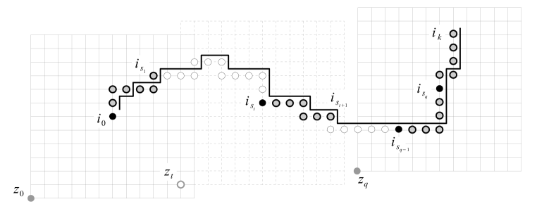
Figure 3: decomposition of $\gamma$

Proof.

Let $\gamma=(i_{0},\ldots,i_{k})$ be a path in $\mathcal{P}_{k}$ with $k\geq N/2$. We decompose $\gamma$ as a concatenation of paths $\gamma_{1}\ast\dots\ast\gamma_{q-1}\ast\gamma_{q}$ with $l(\gamma_{t})\geq N/2$ and each $\gamma_{t}$ contained in a coordinate square $z+[0,N]^{2}$ for some $z\in\mathbb{Z}^{2}$ (see Fig. 3).

If $N$ is even, setting $q=\lfloor\frac{2k}{N}\rfloor$ and $s_{t}=tN/2$ for $t=0,\dots,q$, we define

$$\gamma_{t}=(i_{s_{t-1}},\dots,i_{s_{t}})\hbox{ \ \ for }t=1,\dots,q-1\hbox{ \ \ and \ \ }\gamma_{q}=(i_{s_{q-1}},\ldots,i_{k}).$$ (11)

In this way, setting

$$z_{t}=i_{s_{t-1}}-\left(\frac{N}{2},\frac{N}{2}\right)\hbox{ \ \ for }t=1,\dots,q-1$$

$$z_{q}=i_{s_{q}}-\left(\frac{N}{2},\frac{N}{2}\right),$$

it follows that for any $t=1,\dots q$ $\gamma_{t}$ is a path of length $l(\gamma_{t})$ greater than $N/2$ contained in $z_{t}+[0,N]^{2}$. Since $\{c_{ij}\}\not\in\tilde{\mathcal{B}}_{p}^{1/2}(N)$, the number of antiferromagnetic interactions $\mu(\gamma_{t})$ is less than $l(\gamma_{t})/2$ for any $t$. Hence $\mu(\gamma)\leq k/2$.

If $N$ is odd, we pose $q=\lfloor\frac{2k}{N+1}\rfloor$ and $s_{t}=t(N+1)/2$ for $t=0,\dots,q$; defining the adjacent paths $\gamma_{t}$ as in (11), by setting

$$z_{t}=i_{s_{t-1}}-\left(\frac{N-1}{2},\frac{N-1}{2}\right)\hbox{ \ \ for }t=1,\dots,q-1$$

$$z_{q}=i_{s_{q}-1}-\left(\frac{N-1}{2},\frac{N-1}{2}\right).$$

the result follows as in the previous case. ∎

3.2 Geometry of minimizers

We conclude by stating the results concerning the geometry of the ground states, corresponding to Proposition 9 and Theorem 8 respectively. The main result states that for spin systems not in ${\mathcal{B}}^{1/2}_{p}$ the minimizers of $F$ on large sets are characterized by a majority phase. Remark 14 then assures that this is a generic situation for $N$ large.

Theorem 16.

Let $N\in{\mathbb{N}}$, and let $\{c_{ij}\}$ be a $N$-periodic distribution of ferro/antiferromagnetic interactions such that $\{c_{ij}\}\not\in\tilde{\mathcal{B}}^{1/2}_{p}$. Let $G$ be a Lipschitz bounded open set and let $u_{\varepsilon}$ be a minimizer for $F(\cdot,{1\over\varepsilon}G)$. Then there exists a constant $C$ depending only on $G$ such that either $\overline{\{u_{\varepsilon}=1\}}$ or $\overline{\{u_{\varepsilon}=-1\}}$ is composed of connected components $K_{\varepsilon}^{i}$ such that the length of the boundary of each $K_{\varepsilon}^{i}$ is not greater than $CN$.

As for Theorem 8, the proof relies on the estimate of the length of paths in the interface, which in this case reads as follows.

Proposition 17.

Let $N\in{\mathbb{N}}$, and let $\{c_{ij}\}$ be a $N$-periodic distribution of ferro/antiferromagnetic interactions such that $\{c_{ij}\}\not\in\tilde{\mathcal{B}}^{1/2}_{p}$. Let $D$ be an open bounded subset of $\mathbb{R}^{2}$ such that the distance between the connected components of $\partial q(D)$ is greater than $N/2$. Let $u$ be a minimizer for $F(\cdot,D)$. Then there is no path in the interface $S(u)$ of length greater than $N/2$.

The steps of the proofs are exactly the same as in the random case, by substituting the applications of Lemma 5 with the corresponding applications of Proposition 15 (thus the logarithmic estimates become linear with $N$).

References

- [1] R. Alicandro, A. Braides and M. Cicalese. Phase and anti-phase boundaries in binary discrete systems: a variational viewpoint. Netw. Heterog. Media 1 (2006), 85–107
- [2] R. Alicandro and M.S. Gelli. Local and non local continuum limits of Ising type energies for spin systems. SIAM J. Math. Anal. 48 (2016), 895–931.
- [3] T. Bodineau, D. Ioffe, Y. Velenik, Rigorous probabilistic analysis of equilibrium crystal shapes, J. Math. Phys. 41 (2000) 1033-1098.
- [4] D. Boivin, First passage percolation: the stationary case. Probab. Th. Rel. Fields 86 (1990), 491-499.
- [5] A. Bondy and U.S.R. Murty. Graph Theory. Springer, London, 2008.
- [6] A. Braides. -convergence for Beginners. Oxford University Press, Oxford, 2002.
- [7] A. Braides. Discrete-to-continuum variational methods for lattice systems. Proceedings of the International Congress of Mathematicians August 13–21, 2014, Seoul, Korea (S. Jang, Y. Kim, D. Lee, and I. Yie, eds.) Kyung Moon Sa, Seoul, 2014, Vol. IV, pp. 997–1015
- [8] A. Braides, V. Chiadò Piat, and M. Solci. Discrete double-porosity models for spin systems. Math. Mech. Complex Syst. 4 (2016), 79–102.
- [9] A. Braides and M. Cicalese. Interfaces, modulated phases and textures in lattice systems. Arch. Ration. Mech. Anal., 223 (2017), 977–1017.
- [10] A. Braides, M. Cicalese, and N. K. Yip. Crystalline Motion of Interfaces Between Patterns. J. Stat. Phys. 165 (2016), 274–319.
- [11] A. Braides, MS. Gelli, M. Novaga. Motion and pinning of discrete interfaces. Arch. Ration. Mech. Anal. 195 (2010), 469–498.
- [12] A. Braides, A. Piatnitski. Overall properties of a discrete membrane with randomly distributed defects. Arch. Ration. Mech. Anal., 189 (2008), 301–323.
- [13] A. Braides, A. Piatnitski. Variational problems with percolation: dilute spin systems at zero temperature. J. Stat. Phys. 149 (2012), 846–864.
- [14] A. Braides, A. Piatnitski. Homogenization of surface and length energies for spin systems. J. Funct. Anal. 264 (2013), 1296–1328.
- [15] A. Braides, G. Scilla. Motion of discrete interfaces in periodic media. Interfaces Free Bound. 15 (2013), 451–476.
- [16] A. Braides, G. Scilla. Nucleation and backward motion of discrete interfaces. C. R. Math. Acad. Sci. Paris 351 (2013), 803–806.
- [17] A. Braides and M. Solci. Motion of discrete interfaces through mushy layers. J. Nonlinear Sci. 26 (2016), 1031–1053
- [18] L.A. Caffarelli and R. de la Llave. Interfaces of ground states in Ising models with periodic coefficients. J. Stat. Phys. 118 (2005), 687–719.
- [19] R. Cerf, A. Pisztora, On the Wulff crystal in the Ising model, Ann. Probab. 28 (2000) 947-1017.
- [20] R. Cerf , M. Théret. Law of large numbers for the maximal flow through a domain of in first passage percolation. Trans. Amer. Math. Soc. 363 (2011), 3665-3702.
- [21] L. Euler. Solutio problematis ad geometriam situs pertinentis. Commentarii Academiae Scientiarum Petropolitanae 8 (1741), 128–140.
- [22] O. Garet and R. Marchand, Large deviations for the chemical distance in supercritical Bernoulli percolation. Annals of Probability, 35 (2007), 833–866.
- [23] G.R. Grimmett. Percolation, Springer, 1999.
- [24] M. Wouts. Surface tension in the dilute Ising model. The Wulff construction. Comm. Math. Phys. 289 (2009) 157–204.