Uncertainty in the visibility mask of a survey and its effects on the clustering of biased tracers

Abstract

The forecasted accuracy of upcoming surveys of large-scale structure cannot be achieved without a proper quantification of the error induced by foreground removal (or other systematics like 0-point photometry offset). Because these errors are highly correlated on the sky, their influence is expected to be especially important at very large scales, at and beyond the first Baryonic Acoustic Oscillation (BAO). In this work we quantify how the uncertainty in the visibility mask of a survey, that gives the survey depth in a specific sky area, influences the measured power spectrum of a sample of tracers of the density field and its covariance matrix. We start from a very large set of 10,000 catalogs of dark matter (DM) halos in periodic cosmological boxes, produced with the PINOCCHIO approximate method. To make an analytic approach feasible, we assume luminosity-independent halo bias and an idealized geometry for the visibility mask, that is constant in square tiles of physical length $l$; this should be interpreted as the projection, at the observation redshift, of the angular correlation scale of the foreground residuals. We find that the power spectrum of these biased tracers can be expressed as the sum of a cosmological term, a mask term and a term involving their convolution. The mask and convolution terms scale like $P\propto l^{2}\sigma_{A}^{2}$, where $\sigma_{A}^{2}$ is the variance of the uncertainty on the visibility mask. With $l=30-100$ Mpc$/h$ and $\sigma_{A}=5-20$%, the mask term can be significant at $k\sim 0.01-0.1\ h/$Mpc, and the convolution term can amount to $\sim 1-10$% of the total. The influence of mask uncertainty on power spectrum covariance is more complicated: the coupling of the convolution term with the other two gives rise to several mixed terms, that we quantify by difference using the mock catalogs. These are found to be of the same order of the mask covariance, and to introduce non-diagonal terms at large scales. As a consequence, the power spectrum covariance matrix cannot be expressed as the sum of a cosmological and of a mask term. More realistic settings (realistic foregrounds, luminosity-dependent bias) make the analytical approach not feasible, and the problem requires on the one hand usage of extended sets of mock catalogs, on the other hand detailed knowledge of the correlations among errors in the visibility masks. Our results lie down the theoretical bases to quantify the impact that uncertainties in the mask calibration have on the derivation of cosmological constraints from large spectroscopic surveys.

1 Introduction

Observations of the Cosmic Microwave Background (CMB), e.g. [1, 2], in combination with expansion and LSS probes, have allowed cosmology to enter an age of high precision: presently, CMB observations alone are able to fix the values of cosmological parameters with per-cent accuracy. The $\Lambda$CDM model has passed this tough observational test, and is now considered as the standard model for cosmology, though it is based on the two unknown ingredients of DM and dark energy. The latter manifests itself as a cosmological constant; possible deviations of its equation of state from the simplest $w=-1$ one would give a crucial hint to its nature.

This calls for accurate low-redshift constraints, based on measurements of the large-scale structures (LSS) as traced by observable objects like galaxies. Upcoming surveys, like [DES, 3], Dark Energy Spectroscopic Instrument [DESI, 4, 5]), Extended Baryon Oscillation Spectroscopic Survey (eBOSS), Large Synoptic Survey Telescope [LSST, 6], Euclid [7], Wide-Field Infrared Survey Telescope [WFIRST, 8] and the Square Kilometer Array (SKA), will measure galaxy clustering with sub-percent accuracy. In particular, the BAO feature [9, 10] in the clustering signal provides a standard ruler that will be used to make precision measurements of the geometry of the Universe in the redshift range from $\sim 0$ to $\sim 2$. The large volumes observable at the highest redshifts will allow to probe very large, $\sim$Gpc scales with very low statistical error. This is needed to detect small effects as for example primordial non-Gaussianity or other effects due to General Relativity (GR) or deviations from it [e.g. 11].

With very high statistics, the error budget will be dominated by systematics. On the largest scales, at or beyond the BAO scale, it will become of fundamental importance to keep under control the effect of foregrounds, due both to the zodiacal light and to the Milky Way (galactic extinction and stellar contamination above all). These will act by modulating the survey depth on the sky. A similar modulation will be due to instrumental or survey features, like 0-point offset of photometric calibration [see for instance the calibration of BOSS photometry 12, 13]; in the following, for simplicity we will refer to foreground removal as the process that we are addressing, but our approach is equally valid for these systematics. Careful characterization of foregrounds will make it possible to subtract them. However, the residuals from this subtraction will, in most cases, be highly correlated on the sky, thus mimicking large-scale structure. So, the error on foreground subtraction must be properly propagated to correctly assess the error on parameter estimation.

A great effort has been devoted to understanding the effect of Galactic foreground and foreground removal for the 21-cm line emission in the reionization epoch [e.g. 14, 15], 21-cm intensity mapping survey at low redshift [e.g. 16]. For the LSS an example of foreground analysis is given by the BOSS survey: they analyzed the potential systematic effects on the galaxy observed density [17] finding that the major contributions come from stellar density and Galactic extinction.

In this work we focus on the issue of how the uncertainty in the removal of foregrounds (or other similar systematics, as said above) propagates to the measurement of clustering at the two-point level and to its covariance. The number of galaxies in an observed sample is given, on average, by the integral of the galaxy luminosity function from a luminosity threshold, determined by the survey flux limit, to infinity. In realistic cases, the flux limit is modulated on the sky by foregrounds, and these are typically correlated on large angular scales. A visibility mask will quantify this effect in order to remove it, but this removal will be done with some uncertainty. This will result in a modulation of the luminosity threshold, that will propagate to the number density of observed objects, creating fake large-scale structure.

To address this issue, we have used the approximate method PINOCCHIO [18] to run 10,000 simulations of a box of $1.5\ h^{-1}$ Gpc. We will consider DM halo “mock” catalogs at redshift $z=1$, where it is possible to have observational access to large volumes and the lower level of non linearities allows approximate methods to be more accurate. We use DM halos in place of galaxies as biased tracers of the density field, and their mass in place of galaxy luminosity. This simplification of the procedure is acceptable in this context, as long as clustering on very large scales is considered and halo mass is simply used to implement the effect of a varying “luminosity” threshold. As a note, a one-to-one correspondence between luminosity and mass is equivalent to a simplified halo occupation distribution (HOD) model, as we will comment in section 3.

To derive analytic predictions of the clustering of these mock catalogs, we build a toy model based on the following assumptions. (i) A mass-independent bias scheme is implemented. DM halos and galaxies share the property of having a mass- or luminosity-dependent bias, but this greatly complicates the analytic approach. We implement mass-independent bias by shuffling halo masses among the objects, as explained in section 3. A coincise analysis of the mass-dependent bias case will be outlined in Appendix B. (ii) We consider an idealized geometry for the mask. In a plane-parallel approximation, the plane of the sky is identified with the $x-y$ plane. This is tiled with squares of physical length $l$, and for each tile the residual of foreground subtraction is quantified by drawing a random number from a Gaussian distribution. No correlation among tiles is considered, so the length $l$ is to be interpreted as the projection (in a flat sky approximation), at the observation redshift, of the angular correlation length of the residual foreground.

Using measurements of the power spectrum on the 10,000 mock catalogs (with and without imposing a mask), and comparing them with analytic predictions, we will show that it is possible to fully quantify the impact of the visibility mask on the power spectrum of biased tracers. This can be written as the sum of a pure cosmological term, a pure mask term, and a term involving their convolution. The same computation for the covariance matrix of the power spectrum is much more complicated, because the convolution term gives rise to a long list of mixed terms that are not easy to compute analytically, even in this idealized setting. This leads to the conclusion that the covariance matrix of the power spectrum cannot be simply written as the sum of a cosmology term and a mask term.

The paper is organized as follows. Section 2 is dedicated to the theoretical description of our idealized mask model and its effect on the measurement of $P(k)$. We will analyze all the extra terms in the power spectrum and its covariance due to the presence of this foreground, including its coupling with the cosmological signal. In section 3 we will describe the cosmological mock samples used to test our mask model and a description of the technique used to compute the mask power spectrum and produce masked catalogs. Section 4 will present the results obtained by applying the mask to the mock catalogs, under the assumption of a galaxy bias independent of luminosity. Section 5 will give the main conclusions of the paper. Appendix A reports a more detailed list of all the mixed terms of the power spectrum covariance matrix, while in appendix B we will briefly discuss the case of luminosity-dependent bias, highlighting a possible path for an analytic approach.

2 Power spectrum of biased tracers in the presence of foregrounds

In this section we derive some simple analytical expressions describing the corrections to the power spectrum (and its covariance) of a galaxy sample defined by a given, nominal luminosity threshold $L_{0}$ when some foregrounds induce local variations $\delta L$ to the effective threshold that depend on the position on the sky.

2.1 Luminosity function and galaxy number density

Let us consider a flux-limited sample of galaxies with luminosity function $\bar{\Phi}(L)$, and let $\Phi(\mathbf{x},\,L)dL$ be the galaxy number density at the position $\mathbf{x}$ with luminosity between $L$ and $L+dL$ so that $\bar{\Phi}(L)\equiv\langle\Phi(\mathbf{x},\,L)\rangle$, with $\langle\dots\rangle$ (and the bar) denoting averages over a very large volume. In general, $\Phi(\mathbf{x},\,L)$ cannot be factorized into the product of a luminosity-dependent ($\bar{\Phi}(L)$) and a position-dependent function; if this were the case, the amplitude of clustering would be independent of luminosity. This means that $\Phi(\mathbf{x},\,L)$ encodes the information of luminosity-dependent bias.

If our determination of a galaxy luminosity is not affected by foregrounds, the galaxy number density of a sample of galaxy characterised by the lower luminosity threshold $L_{0}$ will be given by

$$n(\mathbf{x};L_{0})=\int_{L_{0}}^{\infty}dL\,\Phi(\mathbf{x},L)\,,$$ (2.1)

while its mean value will be

$$\bar{n}(L_{0})=\int_{L_{0}}^{\infty}dL\,\bar{\Phi}(L)\,,$$ (2.2)

We can characterize spatial fluctuations in the number density of galaxies of luminosity $L$ by means of the galaxy overdensity $\delta_{\Phi}(\mathbf{x},\,L)$ defined by the relation

$$\Phi(\mathbf{x},\,\,L)=\bar{\Phi}(L)\,[1+\delta_{\Phi}(\mathbf{x},\,L)]\,.$$ (2.3)

For a sample of galaxies with luminosity threshold $L_{0}$ we define instead the overdensity $\delta(\mathbf{x};\,L_{0})$ by means of the relation

$$n(\mathbf{x};\,L_{0})=\bar{n}(L_{0})\,[1+\delta(\mathbf{x};\,L_{0})]\,.$$ (2.4)

It follows that the two overdensities $\delta_{\Phi}(\mathbf{x},\,L)$ and $\delta(\mathbf{x};\,L_{0})$ are related by

$$\bar{n}(L_{0})\,\delta(\mathbf{x};\,L_{0})=\int_{L_{0}}^{\infty}dL\,\bar{\Phi}(L)\,\delta_{\Phi}(\mathbf{x},\,L)\,.$$ (2.5)

In an observed sample, our measurement of the galaxy luminosity $L$ will be influenced by foregrounds. The two most obvious cases are galaxy extinction, that will decrease the observed flux, and zodiacal light, that will increase the sky noise; contamination by field stars or survey features (e.g., seeing conditions from the ground or solar aspect ratio from space), or survey features like modulations of 0-point of photometric calibration are other examples. For a fixed observed flux limit, the true limiting magnitude, and then the true density, will be modulated by these foregrounds, or by any residual of a foreground removal procedure. We expect, with some generality, such residuals to be highly correlated on the sky and we model here, in a very simple way, how this correlation affects the measurement of the galaxy power spectrum and its covariance.

We are interested in studying how a modulation of the intrinsic flux limit propagates to the observed galaxy density and its correlation functions. To this aim, we assume that the effect of residual foregrounds consists in changing locally the luminosity threshold $L_{0}$ by a quantity $\delta L({\boldsymbol{\theta}})$, where ${\boldsymbol{\theta}}$ is a vector that defines the position on the sky. We further assume that such perturbations to $L_{0}$ are small, i.e. $\delta L/L_{0}\ll 1$, and that, as residuals, they have vanishing spatial mean, that is $\langle\delta L({\boldsymbol{\theta}})\rangle=0$, The observed galaxy number density of a sample with nominal threshold $L_{0}$ will then be written as

$$n_{\rm obs}(\mathbf{x};\,L_{0}) =\int_{L_{0}+\delta L({\boldsymbol{\theta}})}^{\infty}dL\,\Phi(\mathbf{x},\,L)\,,$$

$$=n(\mathbf{x};\,L_{0})+\delta n(\mathbf{x};\,L_{0})\,,$$ (2.6)

where the second contribution on the r.h.s., defined as

$$\delta n(\mathbf{x};\,L_{0})=\int^{L_{0}}_{L_{0}+\delta L({\boldsymbol{\theta}})}dL\,\Phi(\mathbf{x},\,L)\,,$$ (2.7)

represents the correction due to the mask foreground residuals. We notice that:

$$\delta n(\mathbf{x};\,L_{0}) =\int^{L_{0}}_{L_{0}+\delta L({\boldsymbol{\theta}})}dL\,\bar{\Phi}(L)\,[1+\delta_{\Phi}(\mathbf{x},\,L)]$$

$$=\int^{L_{0}}_{L_{0}+\delta L({\boldsymbol{\theta}})}dL\,\bar{\Phi}(L)$$

$$+\int^{L_{0}}_{L_{0}+\delta L({\boldsymbol{\theta}})}dL\,\bar{\Phi}(L)\,\delta_{\Phi}(\mathbf{x},\,L)\,.$$ (2.8)

In the last equation, the first contribution on the r.h.s., describes the effect of the fluctuations in luminosity $\delta L({\boldsymbol{\theta}})$ on the mean density and has therefore only an angular dependence. The second contribution, instead, accounts for the effect of the fluctuations in the threshold on the density perturbation and it is therefore expected to be subdominant (although not necessarily negligible).

It is important to stress that, even if $\langle\delta L({\boldsymbol{\theta}})\rangle=0$, we cannot expect that the ensemble average of the correction vanishes, i.e. $\langle\delta n(\mathbf{x};\,L_{0})\rangle=0$, because of the nonlinear dependence on $\delta L({\boldsymbol{\theta}})$. In particular, the mean of the second contribution of equation (2.1) vanishes due to the fact that density perturbations at high redshift are expected to be uncorrelated to any foreground residual, and that $\langle\delta_{\Phi}\rangle=0$ by definition. The first term can be Taylor-expanded:

$$\int^{L_{0}}_{L_{0}+\delta L({\boldsymbol{\theta}})}dL\,\bar{\Phi}(L)\simeq\bar{\Phi}(L_{0})\,\delta L+\frac{1}{2}\frac{d\bar{\Phi}}{dL}(L_{0})(\delta L)^{2}+\dots$$ (2.9)

It is clear that $\langle\delta n(\mathbf{x};\,L_{0})\rangle$ will be non-zero at the second-order in $\delta L({\boldsymbol{\theta}})$. For these reasons, in the definition of the observed galaxy overdensity $\delta_{\rm obs}(\mathbf{x};\,L_{0})$ given by the usual expression

$$n_{\rm obs}(\mathbf{x};\,L_{0})\equiv\bar{n}_{\rm obs}(L_{0})\,\Bigl{[}1+\delta_{\rm obs}(\mathbf{x};\,L_{0})\Bigr{]}\,,$$ (2.10)

the mean value $\bar{n}_{\rm obs}(L_{0})$ does not equal to the true mean density $\bar{n}(L_{0})$.

2.2 The case of luminosity-independent bias

A possible analytical description of galaxy perturbations in the presence of residual foregrounds consists in Taylor-expanding the observed number density $n_{\rm obs}(L_{0})$ in the threshold perturbations $\delta L({\boldsymbol{\theta}})$. We will present some basic results of such exercise in Appendix B. Instead, in what follows we will make the assumption that the quantity $\Phi(\mathbf{x},\,L)$ can be factorized as the product of a luminosity-dependent and a position-dependent function. In terms of equation (2.3):

$$\Phi(\mathbf{x},\,L)\simeq\bar{\Phi}(L)\,[1+\delta_{\Phi}(\mathbf{x})]\,.$$ (2.11)

This factorisation is clearly unphysical, as it amounts to neglecting any dependence of bias on luminosity, but it allows a great simplification of the calculations.

For instance, we have

$$n(\mathbf{x};\,L_{0})=\bar{n}(L_{0})\,[1+\delta(\mathbf{x})]\,,$$ (2.12)

with $\delta(\mathbf{x})=\delta_{\Phi}(\mathbf{x})$. In particular, the corrections due to foregrounds become

$$\delta n(\mathbf{x};\,L_{0})= \int^{L_{0}}_{L_{0}+\delta L({\boldsymbol{\theta}})}dL\,\bar{\Phi}(L)$$

$$+\int^{L_{0}}_{L_{0}+\delta L({\boldsymbol{\theta}})}dL\,\bar{\Phi}(L)\,\delta(\mathbf{x})$$

$$= [1+\delta(\mathbf{x})]\,\int^{L_{0}}_{L_{0}+\delta L({\boldsymbol{\theta}})}dL\,\bar{\Phi}(L)\,.$$ (2.13)

Introducing now the notation

$$\delta n_{\rm mask}({\boldsymbol{\theta}};\,L_{0})=\int^{L_{0}}_{L_{0}+\delta L({\boldsymbol{\theta}})}dL\,\bar{\Phi}(L)$$ (2.14)

for the perturbations in the number density exclusively due to foregrounds (and therefore only dependent on the angle ${\boldsymbol{\theta}}$) we can write the observed galaxy number density, dropping the explicit dependence on $L_{0}$, as

$$n_{\rm obs}(\mathbf{x}) =[1+\delta(\mathbf{x})]\left[\bar{n}+\delta n_{\rm mask}({\boldsymbol{\theta}})\right]\,.$$ (2.15)

The observed density contrast $\delta_{\rm obs}(\mathbf{x})$, accounting for both cosmological perturbations and foregrounds effect is defined as

$$n_{\rm obs}(\mathbf{x})\equiv\bar{n}_{\rm obs}\,[1+\delta_{\rm obs}(\mathbf{x})]\,.$$ (2.16)

Noting that $\bar{n}_{\rm obs}=\bar{n}+\langle\delta n_{\rm mask}({\boldsymbol{\theta}})\rangle$ we have then

$$\bar{n}_{\rm obs}\,[1+\delta_{\rm obs}(\mathbf{x})]=\bar{n}_{\rm obs}\,[1+\delta(\mathbf{x})]\,[1+\delta_{\rm mask}({\boldsymbol{\theta}})]\,,$$ (2.17)

where we introduced the density contrast

$$\delta_{\rm mask}({\boldsymbol{\theta}})\equiv\frac{\delta n_{\rm mask}({\boldsymbol{\theta}})-\langle\delta n_{\rm mask}({\boldsymbol{\theta}})\rangle}{\bar{n}_{\rm obs}}\,.$$ (2.18)

It is important to stress that $\delta_{\rm mask}$ can be seen both as a function of the sky coordinate ${\boldsymbol{\theta}}$ and as a function of space coordinate $\mathbf{x}$, subject to the constraint of being constant along the lines of sight. Finally we can express the observed galaxy density contrast $\delta_{\rm obs}(\mathbf{x})$ in terms of the actual density contrast $\delta(\mathbf{x})$ and the mask-induced relative density corrections $\delta_{\rm mask}(\mathbf{x})$ (expressed as a function of $\mathbf{x}$) as

$$\delta_{\rm obs}(\mathbf{x})=\delta(\mathbf{x})-\delta_{\rm mask}(\mathbf{x})-\delta_{\rm mask}(\mathbf{x})\,\delta(\mathbf{x})\,.$$ (2.19)

Adopting the following convention for the Fourier Transform

$$\delta(\textbf{k})=\frac{1}{(2\pi)^{3}}\int d^{3}\textbf{x}\ e^{i\textbf{k}\cdot\textbf{x}}\delta(\textbf{x})\ ,$$ (2.20)

the perturbed density contrast, eq. (2.19), in Fourier space will read:

$$\delta_{\rm obs}(\textbf{k})= \delta(\textbf{k})-\delta_{\rm mask}\,(\textbf{k})-\int d^{3}\textbf{q}\,\delta(\textbf{q})\,\delta_{\rm mask}(\textbf{k}-\textbf{q})$$

$$= \delta(\textbf{k})-\delta_{\rm mask}(\textbf{k})-\delta_{\rm conv}(\textbf{k})$$ (2.21)

Here we introduced $\delta_{\rm conv}\equiv\delta\,\otimes\,\delta_{\rm mask}$ as the convolution of $\delta(\mathbf{x})$ and $\delta_{\rm mask}(\mathbf{x})$.

It is important to stress that, in our simplified model we can write the observed density contrast $\delta_{obs}$, eq. (2.19), as a function of the independent quantities $\delta$ and $\delta_{mask}$.

2.3 Power Spectrum

The real-space two-point correlation function for the observed overdensity $\delta_{\rm obs}(\mathbf{k})$ can be simply expanded as

$$\langle\delta_{\rm obs}(\mathbf{k}_{1})\,\delta_{\rm obs}(\mathbf{k}_{2})\rangle \!\!\!\!\!\!=\!\!\!\!\!\! \langle\delta(\mathbf{k}_{1})\,\delta(\mathbf{k}_{2})\rangle+\langle\delta_{\rm mask}(\mathbf{k}_{1})\delta_{\rm mask}(\mathbf{k}_{2})\rangle+$$ (2.22)

$$\langle\delta_{\rm conv}(\mathbf{k}_{1})\,\delta_{\rm conv}(\mathbf{k}_{2})\rangle\,,$$

since $\langle\delta\,\delta_{\rm mask}\rangle=\langle\delta\,\delta_{\rm conv}\rangle=\langle\delta_{\rm mask}\,\delta_{\rm conv}\rangle=0$ (they involve averages of either $\delta$ or $\delta_{\rm mask}$). The total, observed power spectrum $P_{\rm obs}(\mathbf{k})$ will therefore be given by:

$$P_{\rm obs}(\mathbf{k})\,=\,P_{\rm cosmo}(k)\,+\,P_{\rm mask}(\mathbf{k})\,+\,P_{\rm conv}(\mathbf{k})\,,$$ (2.23)

where $P_{\rm conv}$ is the convolution of the cosmological and mask power spectra:

$$P_{\rm conv}(\textbf{k})=\int d^{3}\textbf{q}\,P_{\rm mask}(\textbf{q})\,P_{\rm cosmo}(|\textbf{k}-\textbf{q}|)\ .$$ (2.24)

This term is of great importance because it couples the cosmological signal with the noise coming from the mask. Moreover, the integral generates scale mixing, thus transferring power among different scales. The procedure presented above is analogous to that of computing the effect of the variance of the window function of a survey on the cosmological power spectrum [19].

Introducing a simple estimator for the power spectrum such as

$$\hat{P}(k_{i})=\frac{1}{N_{k_{i}}}\sum_{\textbf{q}\in k_{i}}\delta_{\textbf{q}}\delta_{-\textbf{q}}$$ (2.25)

where $\textbf{q}\in k_{i}$ denotes a sum over all modes for which $k=|\mathbf{k}|$ is in the $i$-th bin of size twice the fundamental frequency, $k_{f}=2\pi/L$, of the box, we can define the power spectrum covariance matrix as

$$C_{ij}\equiv{\rm cov}[\hat{P}(k_{i}),\,\hat{P}(k_{j})]=\langle\delta\hat{P}(k_{i})\delta\hat{P}(k_{j})\rangle$$ (2.26)

where $\delta\hat{P}(k_{i})=\hat{P}(k_{i})-\langle\hat{P}(k_{i})\rangle$ is the deviation of the $\hat{P}(k)$, measured in a given realization, from its ensemble average. It is easy to see that the covariance of the observed power spectrum $P_{\rm obs}$, eq. (2.23), can then be written as

$$C_{ij}^{\rm obs} \equiv {\rm cov}(\hat{P}_{\rm obs}(k_{i}),\,\hat{P}_{\rm obs}(k_{j}))$$ (2.27)

$$= {\rm cov}[\hat{P}_{\rm cosmo}(k_{i}),\,\hat{P}_{\rm cosmo}(k_{j})]+{\rm cov}[\hat{P}_{\rm mask}(k_{i}),\,\hat{P}_{\rm mask}(k_{j})]+C_{ij}^{mixed}$$

$$= C_{ij}^{cosm}+C_{ij}^{mask}+C_{ij}^{mixed}\,,$$

i.e., as a sum of the covariance of the cosmological power spectrum, the covariance of the mask power spectrum $P_{\rm mask}(\mathbf{k})$ plus a mixed term accounting for several contributions that can be written as a function of higher order correlation functions of the density field and of the mask:

$$C_{ij}^{mixed} = \langle\hat{P}_{\rm conv}(k_{i})\hat{P}_{\rm conv}(k_{j})\rangle-\langle\hat{P}_{\rm conv}(k_{i})\rangle\langle\hat{P}_{\rm conv}(k_{j})\rangle+$$ (2.28)

$$\langle\hat{P}_{\rm cosmo}(k_{i})\hat{P}_{\rm conv}(k_{j})\rangle-\langle\hat{P}_{\rm cosmo}(k_{i})\rangle\langle\hat{P}_{\rm conv}(k_{j})\rangle+$$

$$\langle\hat{P}_{\rm mask}(k_{i})\hat{P}_{\rm conv}(k_{j})\rangle-\langle\hat{P}_{\rm mask}(k_{i})\rangle\langle\hat{P}_{\rm conv}(k_{j})\rangle+$$

$$\langle\hat{P}_{\rm cosmo}(k_{i})\hat{G}(k_{j})\rangle+\langle\hat{P}_{\rm mask}(k_{i})\hat{G}(k_{j})\rangle+$$

$$\langle\hat{P}_{\rm conv}(k_{i})\hat{G}(k_{j})\rangle+\langle\hat{G}(k_{i})\hat{G}(k_{j})\rangle$$

where $\hat{G}=2\delta_{\mathbf{q}}\delta_{\rm mask,{\mathbf{q}}}-\delta_{\mathbf{q}}\delta_{\rm conv,\mathbf{q}}+\delta_{\rm mask,\mathbf{q}}\delta_{\rm conv,\mathbf{q}}$, with $\mathbf{q}\in k_{i}$. Appendix A presents a more extended version of this covariance term.

There will be a scale at which perturbations $\delta$ and $\delta_{mask}$ are of the same order of magnitude, in which case there is no obvious reason why mixing terms should be small. A full analytical computation of the additional covariance contribution in $C_{ij}^{mixed}$ is discouraging even in the context of our simple model. Instead, to quantify the various terms we will resort to a numerical assessment taking advantage of the large number of DM halo catalogs produced for this project, to which we will add the effect of a mask as explained in the next section.

3 Simulated Catalogs

3.1 Cosmological Catalogs

As mentioned in the Introduction, our choice is to use DM halos in place of galaxies as biased tracers. Moreover, we will use the mass $M$ of the DM halo in place of the galaxy luminosity $L$. In particular, the nominal mass threshold, i.e. the minimal mass defining the halo sample (in absence of foregrounds) will be denoted as $M_{0}$, corresponding to the $L_{0}$ of the previous section. This is equivalent to applying a minimal HOD model [20] with one galaxy per halo and a linear relation between halo mass and luminosity. This is known to be unrealistic, but we considered this approximation proper for the idealised case presented in this paper.

The simulated catalogs we used for all the measurements are DM halo catalogs obtained with the approximate method PINOCCHIO [21, 22, see [23] for a review of approximate methods]. This method is based on (i) generating a linear density field on a grid, as usually done for the initial conditions of an N-body simulation; (ii) estimating the time at which each grid point (or particle) collapses, using a combination of ellipsoidal collapse model and excursion set theory; (iii) grouping together collapsed particles into DM halos with an algorithm that mimics their hierarchical assembly. Displacements of particles (and DM halos) from their initial positions are computed using Lagrangian Perturbation Theory [e.g. 24]. We use the latest version of the code, V4.1, presented in [18], where displacements were computed with LPT up to the third order, resulting in a sizable improvement of the predicted power spectrum: the wavenumber at which the prediction of $P(k)$ drops by 10 per cent, with respect to an N-body simulation run on the same initial conditions, increases from $k=0.1\ h^{-1}\,{\rm Mpc}$ to $\sim 0.3-0.5\ h^{-1}\,{\rm Mpc}$ at redshift 0 or 1. This lack of accuracy is not relevant for the present analysis, that is mostly focused on large scales.

We generated 10,000 realizations of a cubic $1500\ h^{-1}\,{\rm Mpc}$ box, sampled with $1000^{3}$ particles. This is, to out knowledge, the largest set of catalogs of DM halo catalogs ever presented. The cosmological parameters are $\Omega_{m}=0.285$, $\Omega_{\Lambda}=0.715$, $\Omega_{b}=0.044$, $h=0.695$ and $\sigma_{8}=0.285$. We used outputs at $z=1$, where, as mentioned in the introduction, it is possible to have observational access to large scales and PINOCCHIO is more accurate. The particle mass is $M_{\rm p}=2.67\times 10^{11}\ h^{-1}M_{\odot}$.

We will consider a halo sample defined by a mass threshold $M_{0}=50\times M_{\rm p}$. With this choice we have approximately $500,000$ halos in each catalog, corresponding to a number density of $1.5\times 10^{-4}\ h^{3}\,{\rm Mpc}^{-3}$.

3.2 Implementation of the mask toy model

One side of the simulation box will be serving as the field-of-view in a distant-observer approximation. For simplicity we model patches in the sky characterised by a constant, uniform foreground residual as square tiles covering the box side mentioned above. An “effective” threshold for halo detection will then be defined, as a correction for the nominal one $M_{0}$, for the whole volume (along the line-of-sight) behind a given tile. Fig. 1 provides a pictorial representation of our toy model.

Figure 1: Every simulation box containing the halo catalogs is assumed to represent a cosmological volume in the distant-observer approximation. Patches of equal foreground error residual are modelled as square tiles covering the field-of-view, corresponding to one side of the box.

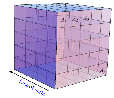
For each halo catalog, we produce a different foreground mask consisting of a correction to the mass threshold $M_{0}$ for each tile across the field-of-view. We will describe the relative variation of threshold as the two-dimensional quantity

$$A({\boldsymbol{\theta}})\equiv\frac{\delta M({\boldsymbol{\theta}})}{M_{0}}\,.$$ (3.1)

Since $A({\boldsymbol{\theta}})$ represents the effect of a residual foreground, we will assume $\langle A({\boldsymbol{\theta}})\rangle=0$, the bracket representing ensemble averages.

We divide the sky plane into square tiles of length $l$, within which $A$ is kept constant, so we can write:

$$A({\boldsymbol{\theta}})=\sum_{i=1}^{N_{t}}A_{i}\Theta_{i}({\boldsymbol{\theta}})$$ (3.2)

where the function $\Theta_{i}({\boldsymbol{\theta}})=1$ if the angular position ${\boldsymbol{\theta}}$ falls inside the $i$-th tile and zero otherwise, and $N_{t}$ is the total number of tiles. The coefficients $A_{i}$ are assigned as independent random numbers, drawn from a Gaussian distribution with standard deviation $\sigma_{A}$, so $A$-values in nearby tiles are uncorrelated. The length $l$ therefore represents the physical correlation length induced by the foreground residual; it will correspond to the projection, at the observation redshift, of an angular correlation scale.

The production of masked halo samples proceeds as follows. First, the DM halo masses provided by PINOCCHIO are modified so as to be continuous. Indeed, the discreteness due to the particle mass can be of the same order of the correction to the mass threshold $\delta M$, leading to spurious effects in the number density that would affect the covariance matrix. This procedure is applied to all halos with more than $30$ particles (we altogether ignore smaller groups); this is smaller than the $50$ particles mass cut mentioned above, because the mask modulation will decrease the mass cut in $\sim$half of the sky tiles. Calling $\alpha$ the logarithmic slope of the DM halo mass function around $M_{0}$ (and computing $\alpha$ from the avaraged mass function of the 10,000 mocks), the halo mass $M$ of a halo made of $N$ particles ($M_{\rm old}=NM_{\rm p}$) is modified as follows:

$$M_{\rm new}=M_{\rm old}\left\{1+r\,\left[\left(\frac{N+1}{N}\right)^{\alpha}-1\right]\right\}^{1/\alpha}$$ (3.3)

where $r$ is a random number between zero and one. Second, in order to remove the mass dependence of halo bias, that invalidates equation (2.11), in each mock catalog halo masses are randomly shuffled among all the halos, thus preserving the halo mass function. In this way, imposing a mass cut is equivalent to a sparse sampling, and halos with different mass cuts will have a similar clustering amplitude. Finally, the catalog is selected by applying the position-dependent mass cut $M_{0}+\delta M({\boldsymbol{\theta}})=M_{0}\,[1+A({\boldsymbol{\theta}})]$.

3.3 Analytical predictions

In terms of the adimensional field $A({\boldsymbol{\theta}})$, and adopting now the halo mass as proxy for the galaxy luminosity, we can rewrite eq. (2.18)

$$\delta_{\rm mask}(\mathbf{x}) = \frac{1}{\bar{n}_{obs}}\,\int^{M_{0}}_{M_{0}\,[1+A({\boldsymbol{\theta}})]}dM\,\bar{\Phi}(M)-\frac{\langle\delta n_{mask}\rangle}{\bar{n}_{obs}}$$ (3.4)

$$= -\frac{M_{0}\,\bar{\Phi}(M_{0})}{\bar{n}}\,A({\boldsymbol{\theta}})+{\mathcal{O}}(A^{2})-\frac{\langle\delta n_{mask}\rangle}{\bar{n}_{obs}}\,,$$

showing that the field $A({\boldsymbol{\theta}})$ represents, modulo a $-$ sign, the overdensity due to the mask, $\delta_{\rm mask}$, up to a multiplicative constant.

From the definiton of $A({\boldsymbol{\theta}})$, eq. (3.2), it is simple to derive explicitly its Fourier transform

$$A_{\mathbf{k}}=\frac{L_{\rm box}l^{2}}{(2\pi)^{3}}\sum_{i}A_{i}e^{ik_{x}x_{i}}e^{ik_{y}y_{i}}j_{0}\left(\frac{k_{x}l}{2}\right)j_{0}\left(\frac{k_{y}l}{2}\right)\delta^{K}_{k_{z},0}$$ (3.5)

where $j_{0}(x)$ is the zeroth-order Bessel function and $\delta^{K}$, the Kronecker symbol. The power spectrum of $A({\boldsymbol{\theta}})$ is given by

$$P_{A}(k_{x},k_{y},k_{z})=\frac{L_{\rm box}l^{2}}{(2\pi)^{3}}k_{f}\sigma_{A}^{2}j_{0}^{2}\left(\frac{k_{x}l}{2}\right)j_{0}^{2}\left(\frac{k_{y}l}{2}\right)\delta_{D}(k_{z})$$ (3.6)

where we took the continuum limit by replacing $\delta^{K}(\textbf{k})/k_{f}^{3}\rightarrow\delta_{D}(\textbf{k})$ for $V\rightarrow\infty$. This term scales as $P_{A}\propto l^{2}\sigma_{A}^{2}$, so that at $k<2\pi/l$ it will grow not only, as expected, with the variance of the residuals but also with the correlation length $l$. Finally, it is equally simple to write down the convolution of the power spectrum $P_{A}(\mathbf{k})$ with a power spectrum $P(k)$ as

$$P_{\rm conv,A}(\mathbf{k}) = \int d^{3}q\,P_{A}(\mathbf{q})\,P_{\rm cosmo}(|\mathbf{k}-\mathbf{q}|)$$ (3.7)

$$= \frac{\sigma_{A}^{2}l^{2}L_{\rm box}k_{f}}{(2\pi)^{2}}\int_{k_{f}}^{k_{max}}dq_{x}\ dq_{y}\ j_{0}^{2}\left(\frac{q_{x}l}{2}\right)j_{0}^{2}\left(\frac{q_{y}l}{2}\right)$$

$$\times P_{\rm cosmo}\left(\sqrt{(k_{x}-q_{x})^{2}+(k_{y}-q_{y})^{2}+k_{z}^{2}}\right)\,.$$

This term, as the previous one, scales as $\propto l^{2}\sigma_{A}^{2}$. The integral in equation (3.7) can be computed numerically, once $P_{\rm cosmo}(k)$ is given. The theoretical prediction for the mask power spectrum makes it possible to analytically compute the convolution term of eq. (2.24), at least at linear order in $A({\boldsymbol{\theta}})$.

$P_{A}(k)$ and $P_{\rm conv,A}(k)$ represent, up to a multiplicative factor, analytical predictions, respectively, for $P_{\rm mask}(k)$ and $P_{\rm conv}(k)$, since, as we will see, corrections due to higher order terms in $A({\boldsymbol{\theta}})$ are small. Of particular interest is the relation between the variance of the mask-induced overdensity, $\sigma_{\rm mask}^{2}\equiv\langle\delta_{\rm mask}^{2}\rangle$, and the variance of the relative error on the mass threshold, $\sigma_{A}^{2}$. To first order in $A$ we have

$$\sigma_{\rm mask}^{2}\simeq\frac{M_{0}^{2}\bar{\Phi}^{2}(M_{0})}{\bar{n}^{2}(M_{0})}\sigma_{A}^{2}\,,$$ (3.8)

where $\bar{\Phi}(M_{0})$ represents now the halo mass function and $\bar{n}(M_{0})$ the number density of objects above the threshold.

3.4 Power spectrum estimators

The power spectrum of the halo catalogs was measured using the estimator of [25], that provides a sophisticated procedure to minimize the impact of aliasing coming from the estimate of density of a set of particles on a $600^{3}$ grid points. All the $k$-bins are multiples of the fundamental frequency of the box, $k_{f}=2\pi/L=0.041\ h^{-1}\,{\rm Mpc}$, while the Nyquist frequency is $k_{Nyq}=N_{g}k_{f}/2=1.256\ h^{-1}\,{\rm Mpc}$, where $N_{g}=600$ is the grid size. The shot noise contribution has always been subtracted. Given that the cosmological density field is isotropic in our case, we present here results for the monopole of the power spectrum; clearly the mask will induce non-zero multipoles, that will contaminate the redshift space distorsion signal; we do not address this point in this paper.

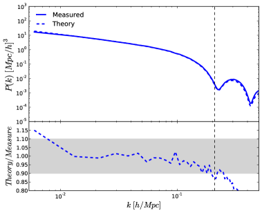
The density field for the estimation of the mask power spectrum, $P_{\rm mask}(k)$, was obtained directly from the two-dimensional field $A({\boldsymbol{\theta}})$ as follows: $\delta_{\rm mask}$ is assumed to be equal to the constant value $A_{i}$ along the whole i-th tile (fig. 1), and the so-defined density field is Fourier-transformed without involving a density estimate on a set of points. As a consequence, the estimation of $P_{\rm mask}(k)$ is not affected by shot noise. As a consistency test, we show in figure (2) the monopole of the mask power spectrum, computed analytically from eq. (3.6) and numerically from 10,000 realisations of the mask $A({\boldsymbol{\theta}})$. The two results are remarkably consistent at large scales, while at small scales the numerical determination shows some overestimate with respect to the analytic one; this is likely due to sampling effects, but such small differences in the range where the term drops are not a concern for what follows.

We expect the mask to affect large scales because of its own geometry: since points behind a given tile are subject to the same effective threshold $L_{0}+\delta L$, they will present some level of induced correlation, even when their separation along the line-of-sight is very large.

Figure 2: Comparison between measured (continuous line) and analytic (dashed line) monopole of the mask power spectrum $P_{\rm mask}(k)$. The black dashed vertical line corresponds to $k=2\pi/l$. The lower panel gives the residuals.

4 Results

The variance of $\delta_{\rm mask}$, $\sigma^{2}_{\rm mask}\equiv\langle\delta_{\rm mask}^{2}\rangle$, gives the magnitude of the effect of the mask on the observed density, and we are interested in the scale range where it is comparable to the variance of the density perturbations $\delta$ (of the same order of the tile length and of the BAO scale). In fact, the limit $\sigma^{2}_{\rm mask}\ll 1$ corresponds to a very good knowledge of the foregrounds, and therefore to a negligible effect of possible residuals, while the opposite limit of large $\sigma^{2}_{\rm mask}$ should describe a situation of poor knowledge of foregrounds that we are expected to avoid.

We will consider the two values $\sigma_{A}=0.05$ and $0.2$ (or errors of $\sim 0.05$ and $\sim 0.20$ magnitudes), corresponding respectively to $\sigma_{mask}=0.07$ and $0.28$. The first value may be a good order of magnitude for a residual foreground (this point will be addressed later), while the second value is very pessimistic and is used to emphasize the effects of foreground removal. We will also assume two different values for the size of the tiles, $l=30$ and $100\ h^{-1}\,{\rm Mpc}$. At $z=1$ and for the cosmological parameters given above, these comoving scales subtend angles of 0.74 and 2.5 degrees. We also tested the case $\sigma_{A}=0.01$; the effect of the mask (for this toy case) is entirely negligible for both the power spectrum and its covariance, so we will not show this case.

4.1 Power Spectrum

Figure 3: Averaged power spectra of mock catalogs. Top panels: tile size = 30 $\times$ 30 Mpc${}^{2}/h^{2}$. Bottom panels: tile size = 100 $\times$ 100 Mpc${}^{2}/h^{2}$. Left panels: $\sigma_{A}=5$%, right panels: $\sigma_{A}=20$%. In all panels the solid lines denote respectively the monopole of total power spectrum (black), cosmological power spectrum (blue), mask power spectrum (red) and convolution term (magenta). These are all measured from catalogs, the last being determined by difference. The dashed red and magenta lines are the theoretical predictions for the mask power spectrum (eq. (3.6)) and the convolution term (eq. (3.7)). The vertical thin lines mark $k=2\pi/l$. The lower plots show the ratio of the various components with respect to the total power spectrum; in this case we only show the measurements from the mocks.

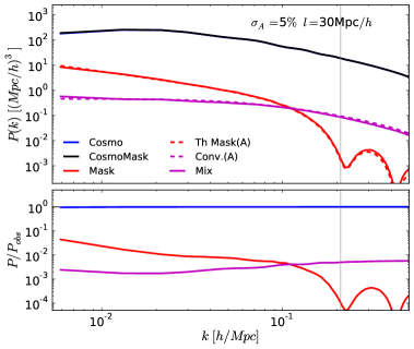
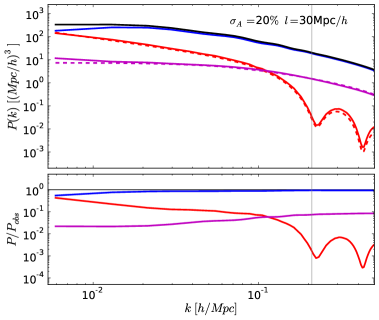
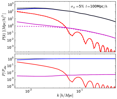
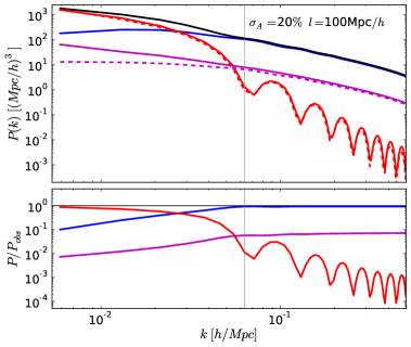
Figure 3 shows the power spectra for all the four considered cases, with $l=30$ and $100\ h^{-1}{\rm Mpc}$ (top and bottom panels) and $\sigma_{A}=0.05$ and $0.2$ (left and right panels). Each panel in the figure is composed by two plots. The upper one shows the monopole of the power spectrum. The coloured lines give the contributions to the power spectrum of eq. (2.23) (denoted by a black line): the blue line is the cosmological power spectrum, $P_{\rm cosmo}(k)$, the red line represents the pure mask contribution, $P_{\rm mask}(k)$, while the magenta line is the convolution term $P_{\rm conv}$ (eq. (2.24)). Solid lines are obtained by measuring the 10,000 mocks as explained in Section 3.4; the convolution term is computed by difference:

$$P_{\rm conv}=P_{\rm obs}-P_{\rm cosmo}-P_{\rm mask}\ .$$ (4.1)

The red and magenta dashed lines represent the theoretical prediction for the power spectrum of the mask, eq. (3.6), and for the cross-term, $P_{\rm conv}$. The latter is obtained from $P_{A}(k)$ with the multiplicative factor from eq. (3.4). In the lower plot of each panel we report the ratio between the components and the observed power spectrum, to highlight the relative size of each contribution. In this case we only report the quantities measured from mocks. Vertical lines in all plots mark $k=2\pi/l$, where the Fourier transform of the mask starts to oscillate. This is equal to $\sim 0.2\ h/$Mpc for $l=30\ h^{-1}$ Mpc, and to $\sim 0.06\ h/$Mpc for $l=100\ h^{-1}$ Mpc.

As anticipated in Figure 2, the contribution of the mask power spectrum (the red line in the plots) is important at large scales, $k<2\pi/l$. Its relevance depends on $l\sigma_{A}$: for $l=30\ h^{-1}$ Mpc it is found to level at about 1 per cent for $\sigma_{A}=5$% and in excess of 10 per cent for $\sigma_{A}=20$%, while for $l=100\ h^{-1}$ Mpc its importance gets increasingly large at large scales even for $\sigma_{A}=5$%, while it dominates at $k<0.03\ h/$Mpc for the higher variance case. At $k>2\pi/l$ the mask is typically negligible, even though the first peaks still get above the 1 per cent level in the high variance case. It is useful to recall that these oscillations are simply the result of our toy model, and therefore they do not necessarily have a real physical meaning.

The contribution of the cross-term does not fall down at small scales, but remains at a fraction of the cosmological power spectrum. At small scales, this fraction is always below the 1 per cent level for $\sigma_{A}=5$%, but is found to be $\sim 10$ per cent in the higher variance case; notably, this fraction scales with $\sigma_{A}$ but not with $l$. The relatively larger contribution of $P_{\rm conv}$ with respect to $P_{\rm mask}$ for $k>2\pi/l$ is the result of the transfer of large-scale power operated by the convolution and does not show the rather artificial oscillations of the latter. At large scales the convolution term is always overtaken by $P_{\rm mask}$, so it never becomes dominant, its relative weight ranging from tenths of per cent to few per cent. Here we notice a small discrepancy between the theoretical prediction for $P_{\rm conv}$ and the measured one at large scales that could be due to the small difference between the theoretical prediction for the mask power spectrum and the measured one at large scales (fig. 2).

The agreement of analytic and measured contributions allows us to be confident in the control of the total power spectrum. In the analysis of the power spectrum covariance we will only use the quantities measured from the 10,000 mock catalogs.

As a concluding remark, the mask power spectrum $P_{\rm mask}(k)$ can easily be important at large scales even when foreground removal is controlled to within a few per cent. The reason lies in the scaling with $(l\sigma_{A})^{2}$: a highly correlated foreground will anyway give a significant contribution to large scales. Conversely, the convolution term gives a roughly constant relative contribution to the power spectrum, that is typically negligible if the uncertainty in the foreground removal is controlled at the few per cent level, but can become important in more pessimistic cases. Because the mask creates power on large scales, within this toy model one could conclude that the BAO scale should be safe at the per cent level if good control, to the few per cent level, is achieved on foreground removal. We will get back to this point in the Conclusions.

4.2 Covariance

Figure 4: Averaged diagonal components of the covariance matrix of mock catalogs. Top panels: tile size = 30 $\times$ 30 $h^{-1}\,{\rm Mpc}$. Bottom panels: tile size = 100 $\times$ 100 $h^{-1}\,{\rm Mpc}$. Left panels: $\sigma_{A}=5$%, right panels: $\sigma_{A}=20$%. In all panels the solid lines denote respectively the variance of the total power spectrum (black), cosmological power spectrum (blue), mask power spectrum (red) and all mixed terms (magenta). These are determined by difference, dotted lines denote negative values. The vertical thin lines mark $k=2\pi/l$. The lower plots show the ratio of the various components with respect to the total power spectrum. In all figures, the vertical ticks denote the wavenumbers used to show the off-diagonal terms in Figure 5.

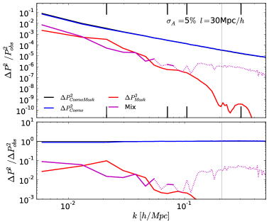
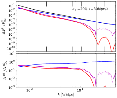
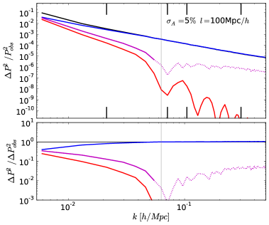
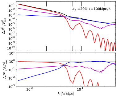
Figure 4 shows the variance of the measured power spectra (all the different components), divided by the measured power spectrum squared, $\Delta P^{2}/P_{\rm obs}^{2}$. For a purely cosmological Gaussian field it would correspond simply to the inverse of the number of available $k$-modes $1/N_{\mathbf{k}}$; in fact, we checked that our cosmological term is very similar to the Gaussian prediction. Here, the magenta curve represents the mixed mask-cosmology contribution; we recall that $C_{ij}^{\rm mixed}$ is not simply the covariance of the convolution $P_{\rm conv}$, but includes a variety of different combinations of cosmological and error residuals perturbations, in addition to shot-noise. The mixed term is obtained as the difference:

$$\Delta P_{\rm mixed}^{2}=\Delta P_{\rm obs}^{2}-\Delta P_{\rm cosmo}^{2}-\Delta P_{\rm mask}^{2}\,,$$ (4.2)

since all components on the r.h.s. can be measured independently. The dotted parts of these curves denote the place where the mixed term gets negative and then oscillates around zero. In this region the subtraction of shot noise induces an uncertainty that is larger than the signal seeked for (the measurement of the mask power spectrum is not affected by shot noise, so we can detect a much lower signal). The lower plots show the contribution of each component with respect to the total one, measured on masked mock catalogs.

Like the power spectrum case, $k=2\pi/l$ marks the scale above which the pure mask term is important. Comparing the contribution of different components to the total power spectrum variance we notice that the pure mask component $\Delta P_{\rm mask}^{2}$ and the mixed one $\Delta P_{\rm mixed}^{2}$ present a similar scale-dependence and comparable amplitudes, at least in the large-scale range where the mixed terms can be measured. Starting from the configuration with $\sigma_{A}=0.05$ and $l=30\ h^{-1}\,{\rm Mpc}$, the pure mask and mixed terms contribute to the total variance by a few per cent. Mixed terms are so small in the first BAO region that they can hardly be measured even with this statistics. So the contribution of mask terms is modest and limited to large scales. Things become pretty different when $\sigma_{A}$ and $l$ are increased. The high variance case gives contributions of mask and mixed terms well in excess of 10 per cent at the BAO scale, that become dominant at the largest scales sampled by the boxes. In the large tile size case the mixed terms get to the 10 per cent level even with the modest mask variance of 5%, while in the high variance, large tile size case the covariance is completely dominated by the mask term on large scales, while the mixed term remains above the 10 per cent level but still larger than the cosmic variance. This is the only case where the mixed terms give a measurable contribution at scales smaller ($k$ higher) than $2\pi/l$; like the convolution term in the power spectrum, they give a relevant and non-oscillating small-scale contribution.

This analysis only shows the diagonal of the covariance matrix. Off-diagonal terms of the covariance matrix are of great importance, because they get mixed with the diagonal term during the matrix inversion necessary to determine the precision matrix that enters the likelyhood function. We now consider how uncertainties in foreground subtraction affect the covariance between different wavenumbers by studying the cross-correlation coefficients defined as:

$$r_{ij}=\frac{C_{ij}}{\sqrt{C_{ii}^{obs}C_{jj}^{obs}}}\,.$$ (4.3)

where $C_{ij}$ is defined by eq. (2.26). These are shows in figure 5 for some relevant values of $k_{j}$ ($0.02$, $0.07$, $0.1$ and $0.31\ h/$Mpc), as a function of $k_{i}$. These $k$-values span the range from very large to non-linear scales, and are marked in Figure 4 as vertical ticks.

Figure 5: Correlation coefficient: Top panels: tile size = 30 $\times$ 30 $h^{-1}\,{\rm Mpc}$. Bottom panels: tile size = 100 $\times$ 100 $h^{-1}\,{\rm Mpc}$. The color code is the same of the previous figures.

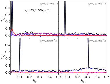
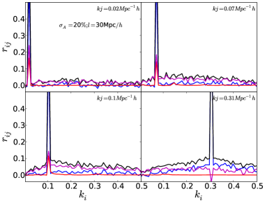
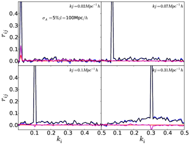
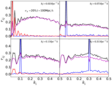
The figure shows how contributions to the normalized covariance due to mask and mixed terms are negligible in the first configuration with $\sigma_{A}=5$% and $l=30h^{-1}\,{\rm Mpc}$. Off-diagonal terms are small in all cases, the cosmological one being appreciable at the highest $k_{j}$. However, in the smallest $k_{j}$ bin the mixed terms give a roughly constant contribution of few per cent. Increasing the scale $l$, we do not notice a larger impact of mask or mixed terms as we did for the diagonal; it seems that off-diagonal terms become significant at $k\ll 2\pi/l$, a regime that is not yet reached at $k=0.02\ h/$Mpc in this case. But when $\sigma_{A}=0.2$, off-diagonal terms become very significant, amounting to 5 per cent for $l=30h^{-1}\,{\rm Mpc}$ and are in excess of 20 per cent for $l=100h^{-1}\,{\rm Mpc}$, independently of scale. In this latter (rather extreme) case the structure of the power spectrum covariance matrix is strongly modified; clearly, an inversion of this matrix without proper account of off-diagonal terms would lead to large errors in parameter determination.

5 Conclusions

We have addressed the problem of how the uncertainty in the removal of foregrounds, in an observational survey of biased tracers like galaxies, propagates to the measurement of the cosmological power spectrum and its covariance matrix. For this first investigation we have decided to use a simplified setting, so as to be able to formulate analytic solutions for the two-point statistics. We have used DM halos as biased tracers, and their mass as a proxy of galaxy luminosity, as in a simplified HOD where each halo is populated by a single galaxy. To this aim, we have produced a very large set of 10,000 realizations of $1.5\ h^{-1}$ Gpc boxes, and extracted DM halos from these volumes at redshift $z=1$ using the PINOCCHIO approximate method. This is, to our knowledge, the largest set of cosmological catalogs of DM halos. We have neglected luminosity- (mass-)dependent bias by randomly shuffling masses among DM halos in each catalog, so as to preserve their mass function. As for the foreground, we have constructed a simple toy model where, in a plane-parallel approximation, the $x-y$ plane of the box is tiled in squares of side $l$, that are characterised by a Gaussian residual foreground of variance $\sigma_{A}^{2}$ that propagates to the density through a modulation of the mass limit $M_{0}$; residuals in different tiles are uncorrelated, so $l$ should be interpreted as the projection, at the observation redshift, of an angular correlation scale of the foreground. The chosen values of 30 and 100 $h^{-1}\,{\rm Mpc}$ are subtended, at $z=1$, by angles of 0.74 and 2.5 degrees respectively.

The main conclusions of our analysis can be summarized as follows:

(1) The residuals of foreground subtraction (“mask”) enter the power spectrum of masked catalogs as two terms, the power spectrum of the mask and its convolution with the cosmological power spectrum. This is similar to what happens when a survey geometry is applied to a cosmological volume.

(2) The mask term is significant at $k<2\pi/l$, while the convolution term is usually smaller in this scale range, but can still be significant at smaller scales due to its scale mixing. Mask and convolution terms scale as $l^{2}\sigma_{A}^{2}$, implying that large correlation lengths of the mask residuals may have a significant effect on large scales even when the foreground removal is controlled to within a few per cent.

(3) Analytic estimations of mask and mixed power spectrum terms give results consistent with those measured from mocks, giving confidence on the level of control of the various terms.

(4) The power spectrum covariance matrix contains not only the cosmological and mask contributions, but also several, additional terms due the coupling of the convolution term with both mask and cosmology. The sum of all these terms can only be determined by difference of measurements of masked mocks, cosmological mocks and pure mask.

(5) Mask and mixed terms are found to have similar effect on the power spectrum covariance matrix. A 5% accuracy on foreground removal guarantees a modest impact of these terms, with the exception of $k\ll 2\pi/l$ modes, where they can significantly contribute to the diagonal. In this case mixed terms give a roughly constant contribution to non-diagonal elements of the covariance matrix. The higher variance case of $\sigma_{A}=20$% shows a dramatic impact on the structure of the covariance matrix.

(6) As a consequence of the relevance of mixed terms, a simple modeling of the covariance matrix as the sum of a pure cosmological term and a cosmology-independent term due to the mask appears to be an oversimplification, as the mixed terms couple cosmology and mask.

As long as BAO is the main target of an observational project, the results presented in this paper point to the conclusion that a $\sim 5$% error in foreground removal should guarantee a modest impact of the mask on parameter estimation. Indeed, due to the $l^{2}\sigma_{A}^{2}$ scaling, signals with smaller correlation scales will have little impact, while a large correlation length $l$ will mostly impact on larger scales (we limited our analysis to correlation lengths that are subtended, at $z=1$, by relatively small angles because of the constraints on the box size). These errors can be compared to estimated errors in foreground removal or photometric calibration. Clearly, the case $\sigma_{A}=20$% is pessimistic, and has been shown only to illustrate the effect of the mask. Photometric calibration can be controlled to the millimag level [12], so its induced errors will likely be negligible. Conversely, Galaxy extinction is know to the few per cent level [26, 27, 28] and zodiacal light can have a similar uncertainty far from the ecliptic [29]. $\sigma_{A}=5$% can then be considered a realistic order of magnitude for the largest contribution to the visibility mask uncertainty. However, this conclusion is based on a very idealized setting, so it should be taken only as an indication, before tests with much more realistic mocks and masks are performed. On the one hand, this toy model is mixing modes on the whole box length; in a realistic survey a redshift bin would span a smaller comoving distance on the line of sight, and this would reduce the impact of mixed terms. On the other hand, a more complex mask like galactic extinction, having power on a range of scales, may easily have a stronger impact than our toy model; luminosity-dependent bias would also add to the covariance in a way that needs to be addressed.

To reduce the impact of a foreground to a desired level, one can of course work to improve the modeling of the foreground and of its correlated residuals. But another way to reduce this impact is to work on the estimator of the two- point statistics, with the aim of minimizing the impact of the residuals. This has been done, in preparation to the DESI survey [4, 5]) by [30] for the two-point correlation function, and by [31] for the power spectrum. In the first paper the authors modify the estimator of the correlation function to remove the angular mode contaminated by the incompleteness due to fiber assignment; in the second paper they investigate different methods to define the survey mean density, in particulare taking into accunt the fiber assignment coverage.

Two conclusions from the tests we have presented are robust. Firstly, the impact of foreground removal is of dramatic importance to properly sample the large scales beyond the BAO. This is expected: foregrounds, especially the zodiacal light, are correlated on large angular scales, that are projected to very large scales where the clustering signal is weak. But the scaling with $l\sigma_{A}$ shows that mode coupling gives a large weight to large-scale correlations, making the control of residual errors of great importance. It is convenient to recall that measurement of non-Gaussianity with error on the ${f_{NL}}$ smaller than unity, or effects of scale-dependent growth related to modified gravity, should be revealed at scales beyond the power spectrum peak; therefore the effect of foreground residuals are crucial for these measurements. Secondly, a poor control of foregrounds can lead to great changes in the covariance matrix. In particular, a significant presence of non-diagonal terms has deep consequences in the the ability to invert the covariance matrix and produce correct estimations of cosmological parameters and their errorbar. Control of foregrounds to the few per cent level is confirmed to be of paramount importance for large-scale structure.

Appendix A Covariance Mix Terms

Eq. (2.28) shows all the terms that come from the coupling of the cosmological signal with the mask. The mixed terms

$$C_{ij}^{obs}\supset \langle\hat{P}_{\rm cosmo}(k_{i})\hat{G}(k_{j})\rangle+\langle\hat{P}_{\rm mask}(k_{i})\hat{G}(k_{j})\rangle+$$ (A.1)

$$\langle\hat{P}_{\rm conv}(k_{i})\hat{G}(k_{j})\rangle+\langle\hat{G}(k_{i})\hat{G}(k_{j})\rangle$$

are written in implicit form. We recall that

$$\hat{G}=\delta_{\mathbf{q}}\delta_{\rm mask,{\mathbf{q}}}-\delta_{\mathbf{q}}\delta_{\rm conv,\mathbf{q}}+\delta_{\rm mask,\mathbf{q}}\delta_{\rm conv,\mathbf{q}}\ ,$$ (A.2)

where $\delta$, $\delta_{\rm mask}$ and $\delta_{\rm conv}$ are given in section (2). Inserting eq. (A.2) into eq. (A.1) we end up with four mix terms that we call $C_{\rm mix}^{i}$, with $i=1...4$. Let’s start with the first contribution that come from the first line of eq. (A.1):

$$C_{\rm mix}^{1} = \frac{1}{N_{k_{i}}N_{k_{j}}}\sum_{\mathbf{q}\in k_{i}}\sum_{\mathbf{p}\in k_{j}}\langle\delta_{\mathbf{p}}\delta_{-\mathbf{p}}\delta_{\rm mask,\mathbf{q}}\delta_{\rm conv,-\mathbf{q}}-\delta_{\mathbf{p}}\delta_{-\mathbf{p}}\delta_{\mathbf{q}}\delta_{\rm conv,-\mathbf{q}}-$$ (A.3)

$$\delta_{\mathbf{p}}\delta_{-\mathbf{p}}\delta_{\mathbf{q}}\delta_{\rm mask,-\mathbf{q}}\rangle=$$

$$\frac{1}{N_{k_{i}}N_{k_{j}}}\sum_{\mathbf{q}\in k_{i}}\sum_{\mathbf{p}\in k_{j}}\int d^{3}s\ \langle\delta_{\mathbf{p}}\delta_{-\mathbf{p}}\delta_{-\mathbf{q}}\rangle\langle\delta_{\rm mask,\mathbf{q}}\delta_{\rm mask,-\mathbf{q}}\rangle+\rm{cc}\ =0\ ,$$

for all $\mathbf{q}$ different from zero, with cc for complex conjugate. For the same reason $C^{2}_{\rm mix}=0=C^{3}_{\rm mix}$. The only non zero contribution is:

$$C_{\rm mix}^{4} = \frac{1}{N_{k_{i}}N_{k_{j}}}\sum_{\mathbf{q}\in k_{i}}\sum_{\mathbf{q}\in k_{j}}[\langle\delta_{\rm mask,\mathbf{q}}\delta_{\rm mask,\mathbf{p}}\delta_{\rm conv,-\mathbf{q}}\delta_{\rm conv,-\mathbf{p}}-$$ (A.4)

$$\delta_{\rm mask,\mathbf{q}}\delta_{\mathbf{p}}\delta_{\rm conv,-\mathbf{q}}\delta_{\rm conv,-\mathbf{p}}-\delta_{\rm mask,\mathbf{q}}\delta_{\mathbf{p}}\delta_{\rm conv,-\mathbf{q}}\delta_{\rm mask,-\mathbf{p}}-$$

$$\delta_{\mathbf{q}}\delta_{\rm mask,\mathbf{p}}\delta_{\rm conv,-\mathbf{q}}\delta_{\rm conv,-\mathbf{p}}+\delta_{\mathbf{q}}\delta_{\mathbf{p}}\delta_{\rm conv,-\mathbf{q}}\delta_{\rm conv,-\mathbf{p}}+$$

$$\delta_{\mathbf{q}}\delta_{\mathbf{p}}\delta_{\rm mask,-\mathbf{p}}\delta_{\rm conv,\mathbf{q}}-\delta_{-\mathbf{q}}\delta_{\rm mask,\mathbf{q}}\delta_{\rm mask,\mathbf{p}}\delta_{\rm conv,-\mathbf{p}}+$$

$$\delta_{\mathbf{q}}\delta_{\rm mask,-\mathbf{q}}\delta_{\mathbf{p}}\delta_{\rm conv,-\mathbf{p}}+\delta_{\mathbf{q}}\delta_{\rm mask,-\mathbf{q}}\delta_{\mathbf{p}}\delta_{\rm mask,-\mathbf{p}}\rangle]=$$

$$\frac{1}{N_{k_{i}}N_{k_{j}}}\sum_{\mathbf{q}\in k_{i}}\sum_{\mathbf{p}\in k_{j}}\Bigl{\{}\int d^{3}s_{1}d^{3}s_{2}\ \langle\delta_{-\mathbf{q}}\delta_{-\mathbf{p}}\rangle\langle\delta_{\rm mask,\mathbf{q}}\delta_{\rm mask,\mathbf{p}}\delta_{\rm mask,-\mathbf{q}+\mathbf{s}_{1}}\delta_{\rm mask,-\mathbf{p}+\mathbf{s}_{2}}\rangle+$$

$$\qquad\qquad\qquad\quad\int d^{3}s_{1}d^{3}s_{2}\ \langle\delta_{\mathbf{q}}\delta_{\mathbf{p}}\delta_{-\mathbf{q}}\delta_{-\mathbf{p}}\rangle\langle\delta_{\rm mask,-\mathbf{q}+\mathbf{s}_{1}}\delta_{\rm mask,-\mathbf{p}+\mathbf{s}_{2}}\rangle+$$

$$\qquad\qquad\qquad\quad\langle\delta_{\mathbf{q}}\delta_{\mathbf{p}}\rangle\langle\delta_{\rm mask,-\mathbf{q}}\delta_{\rm mask,-\mathbf{p}}\rangle\Bigr{\}}$$

As we can see from the previous relations, the mixed terms are convolutions of high order correlators of both cosmological and mask fields.

It is possible to further expand the expressions, considering that all the 4-point correlators can be written in the form:

$$\langle\delta_{1}\delta_{2}\delta_{3}\delta_{4}\rangle=\langle\delta_{1}\delta_{2}\delta_{3}\delta_{4}\rangle_{\rm connected}+\langle\delta_{1}\delta_{2}\rangle\langle\delta_{3}\delta_{4}\rangle+\rm{perm}.\ .$$ (A.5)

We expect that the cosmological connected part are equal to zero, but we can not assume that the same is valid for the mask connected part.

Appendix B Realistic galaxy bias

In section (2) we made the simplifying assumption that the quantity $\Phi(\mathbf{x};L)$ can be factorized into luminosity-dependent and position-dependent functions (equation 2.11) This condition simplifies the calculations, but it is clearly an approximation sincees it implies luminosity-independent bias. In this section we show how to include a more realistic bias description. We will then compare the predictions for the observed power spectra with the “simplified” condition. As in the main text, we will use halo mass as a proxy for luminosity.

Let us consider the number density of halos with mass greater than the nominal threshold $M_{0}$ to be given by

$$n(\mathbf{x},M_{0})=\int_{M_{0}}^{\infty}dM\ \Phi(\mathbf{x};M)\ ,$$ (B.1)

then the observed number density, after the mask perturbation is

$$n^{obs}(\mathbf{x};M_{0})=\int_{M_{0}\,[1+A({\boldsymbol{\theta}})]}^{\infty}dM\ \Phi(\mathbf{x};M)\,.$$ (B.2)

For small perturbations to the mass threshold, i.e. $\sigma_{A}\lesssim 1$, we can Taylor-expand $n^{obs}$ with respect to $A({\boldsymbol{\theta}})$ to get

$$n^{obs}(\textbf{x};M_{0}) = n(\textbf{x},M_{0})+\frac{\partial n^{obs}}{\partial A}\Bigr{|}_{A=0}A$$ (B.3)

$$+\frac{1}{2}\frac{\partial^{2}n^{obs}}{\partial A^{2}}\Bigr{|}_{A=0}A^{2}+\mathcal{O}(A^{3})\ .$$

that we can formally express as

$$n^{obs}(\mathbf{x},M_{0}) = n(\mathbf{x},M_{0})+n^{(1)}(\mathbf{x},M_{0})A({\boldsymbol{\theta}})$$ (B.4)

$$+n^{(2)}(\mathbf{x},M_{0})A^{2}({\boldsymbol{\theta}})+\mathcal{O}(A^{3})\ ,$$

where

$$n^{(1)}(\mathbf{x},M_{0}) \equiv \frac{\partial n}{\partial(\ln M_{0})}$$ (B.5)

$$n^{(2)}(\mathbf{x},M_{0}) \equiv \frac{1}{2}\frac{\partial^{2}n}{\partial(\ln M_{0})^{2}}\ .$$ (B.6)

We can now expand in $A$ the halo density contrast, defined as

$$\delta_{h}^{obs}(\mathbf{x},M_{0})\equiv\frac{n^{obs}(\mathbf{x},M_{0})}{\bar{n}^{obs}(\mathbf{x},M_{0})}-1\ ,$$ (B.7)

and obtain

$$\delta_{h}^{obs} = \delta_{h}(1-\frac{1}{2}C_{2}\sigma_{A}^{2})+C_{1}A+(C_{1}\delta_{h}+\tilde{\epsilon})A$$ (B.8)

$$+\frac{1}{2}C_{2}(A^{2}-\sigma_{A}^{2})+\frac{1}{2}(C_{2}\delta_{h}+2C_{1}\tilde{\epsilon}+\tilde{\eta})A^{2}$$

$$+\mathcal{O}(A^{3})\ .$$

where $\delta_{h}$ is the cosmological halo density contrast and where we defined

$$C_{1}(M_{0}) \equiv \frac{\partial\ln\bar{n}}{\partial\ln M_{0}}$$ (B.9)

$$C_{2}(M_{0}) \equiv \frac{M_{0}^{2}}{\bar{n}}\frac{\partial^{2}\bar{n}}{\partial M_{0}^{2}}$$ (B.10)

$$\tilde{\epsilon} \equiv M_{0}\frac{\partial\delta_{h}}{\partial M_{0}}$$ (B.11)

$$\tilde{\eta} \equiv M_{0}^{2}\frac{\partial^{2}\delta_{h}}{\partial M_{0}^{2}}\ .$$ (B.12)

It is easy to see that if eq. (2.11) holds, then $\tilde{\eta}=\tilde{\epsilon}=0$ and the density contrast reduces to the form of eq. (2.19). From equation B.8, one can show that the two-point correlation function in Fourier space is given by

$$\langle\delta_{\mathbf{k}_{1}}^{obs}\delta_{\mathbf{k}_{2}}^{obs}\rangle = \delta_{D}(\mathbf{k}_{12})P_{\delta\delta}(k_{1})(1-C_{2}\sigma^{2}_{A})+\langle A_{\mathbf{k}_{1}}A_{\textbf{k}_{2}}\rangle$$ (B.13)

$$+\int d^{3}q[P_{\delta\delta}(q)+2C_{1}P_{\delta\tilde{\epsilon}}(q)+C^{2}_{1}P_{\tilde{\epsilon}\tilde{\epsilon}}(q)]$$

$$\times\langle A_{\mathbf{k}_{1}-\mathbf{q}}A_{\mathbf{k}_{1}+\mathbf{q}}\rangle$$

$$+\frac{1}{2}[C_{2}P_{\delta\delta}(k_{1})+2C_{1}P_{\delta\tilde{\epsilon}}(k_{1})+C_{1}^{3}P_{\tilde{\epsilon}\tilde{\eta}}(k_{1})]$$

$$\times\int d^{3}q\langle A_{\mathbf{q}}A_{\mathbf{k}_{12}-\mathbf{q}}\rangle$$

$$+(\mathbf{k}_{1}\leftrightarrow\mathbf{k}_{1})+\mathcal{O}(A^{3})\ .$$

Since we are interested in a comparison with eq. (2.23), using eq. (2.21) with $\delta^{obs}$ from eq. (B.8) we obtain the monopole of the observed power spectrum to be given by

$$P_{0}^{obs} = P_{\delta\delta}(1-C_{2}\sigma_{A}^{2})+P_{AA,0}(k)$$ (B.14)

$$+\int d^{3}q[P_{\delta\delta}(q)+2C_{1}P_{\delta\tilde{\epsilon}}(q)+C^{2}_{1}P_{\tilde{\epsilon}\tilde{\epsilon}}(q)]P_{AA,0}(|\mathbf{q}-\mathbf{k}|)$$

$$+[C_{2}P_{\delta\delta}(k_{1})+2C_{1}P_{\delta\tilde{\epsilon}}(k_{1})+C_{1}^{3}P_{\tilde{\epsilon}\tilde{\eta}}(k_{1})]\sigma_{A}^{2}$$

$$+\mathcal{O}(A^{3})\ ,$$

where

$$P_{AA,0}(k)=\frac{k_{f}^{3}}{V_{p}(k)}\int_{k}d^{3}\textbf{q}\langle|A_{\textbf{q}}|^{2}\rangle$$ (B.15)

is the monopole of the mask power spectrum. The main difference with (2.23), is given by the presence of the power spectra $P_{\delta\tilde{\epsilon}}$, $P_{\delta\tilde{\eta}}$ and $P_{\tilde{\eta}\tilde{\eta}}$, all dependent on derivatives of the density contrast $\delta_{h}$. Considering a local bias expansion as $\delta_{h}=\sum_{n}b_{n}(M)\delta_{m}^{n}$ these additional terms could be expressed in terms of derivatives of the halo bias functions $b_{n}(M)$.

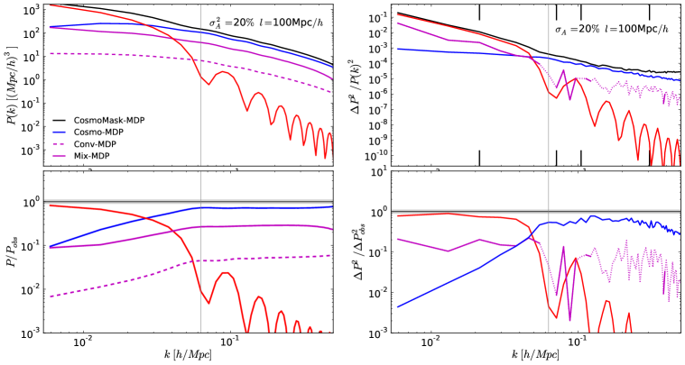
A modulation of the mass threshold implies a different halo selection, and then a different bias. Because the relation between bias and threshold halo mass is not linear, we expect that the bias of halos subject to a mask $A({\boldsymbol{\theta}})$ will be different from the bias of unmasked halos, even when $\langle A({\boldsymbol{\theta}})\rangle=0$. As a consequence, we expect the masked and unmasked catalogs not to match at small scales, as they do in Figure 3.

We will not go into the computation details of the full covariance matrix, because we can directly use mocks to see the effect of introducing the halo bias (fig. (6)). In this figure we show all the power spectrum and variance components; “MDP”(Mass Dependent Bias) marks the terms obtained by using the original DM halo masses, without removing the mass dependency of bias. As expected, at small scales we observe a difference of few percent between the cosmological and the masked power spectrum, due to the mass bias. The same effect is observable in the power spectrum variance at the same scales. Of course this makes the estimation of the convolution term of the power spectrum, and the of mixed terms in the covariance matrix, more complicated. In the figure we show again as magenta lines these terms computed by difference as in the main text, but the large difference between the measurement of the convolution term in the power spectrum and its theoretical prediction shows that there is a problem.

Figure 6: Averaged power spectra and variance components without mass bias removal. Color code is the same of figures (3, 4).

References

- [1] Planck Collaboration, P. A. R. Ade, N. Aghanim, M. Arnaud, M. Ashdown, J. Aumont et al., Planck 2015 results. XIII. Cosmological parameters, ArXiv e-prints (Feb., 2015) , [1502.01589].
- [2] E. Komatsu, K. M. Smith, J. Dunkley, C. L. Bennett, B. Gold, G. Hinshaw et al., Seven-year Wilkinson Microwave Anisotropy Probe (WMAP) Observations: Cosmological Interpretation, ApJS 192 (Feb., 2011) 18, [1001.4538].
- [3] Dark Energy Survey Collaboration, T. Abbott, F. B. Abdalla, J. Aleksić, S. Allam, A. Amara et al., The Dark Energy Survey: more than dark energy - an overview, MNRAS 460 (Aug., 2016) 1270–1299, [1601.00329].
- [4] D. Schlegel, F. Abdalla, T. Abraham, C. Ahn, C. Allende Prieto, J. Annis et al., The BigBOSS Experiment, ArXiv e-prints (June, 2011) , [1106.1706].
- [5] M. Levi, C. Bebek, T. Beers, R. Blum, R. Cahn, D. Eisenstein et al., The DESI Experiment, a whitepaper for Snowmass 2013, ArXiv e-prints (Aug., 2013) , [1308.0847].
- [6] LSST Science Collaboration, P. A. Abell, J. Allison, S. F. Anderson, J. R. Andrew, J. R. P. Angel et al., LSST Science Book, Version 2.0, ArXiv e-prints (Dec., 2009) , [0912.0201].
- [7] R. Laureijs, J. Amiaux, S. Arduini, J. . Auguères, J. Brinchmann, R. Cole et al., Euclid Definition Study Report, ArXiv e-prints (Oct., 2011) , [1110.3193].
- [8] J. Green, P. Schechter, C. Baltay, R. Bean, D. Bennett, R. Brown et al., Wide-Field InfraRed Survey Telescope (WFIRST) Final Report, ArXiv e-prints (Aug., 2012) , [1208.4012].
- [9] D. J. Eisenstein, I. Zehavi, D. W. Hogg, R. Scoccimarro, M. R. Blanton, R. C. Nichol et al., Detection of the Baryon Acoustic Peak in the Large-Scale Correlation Function of SDSS Luminous Red Galaxies, ApJ 633 (Nov., 2005) 560–574, [astro-ph/0501171].
- [10] K. S. Dawson, D. J. Schlegel, C. P. Ahn, S. F. Anderson, É. Aubourg, S. Bailey et al., The Baryon Oscillation Spectroscopic Survey of SDSS-III, AJ 145 (Jan., 2013) 10, [1208.0022].
- [11] L. Amendola, S. Appleby, A. Avgoustidis, D. Bacon, T. Baker, M. Baldi et al., Cosmology and Fundamental Physics with the Euclid Satellite, ArXiv e-prints (June, 2016) , [1606.00180].
- [12] N. Padmanabhan, D. J. Schlegel, D. P. Finkbeiner, J. C. Barentine, M. R. Blanton, H. J. Brewington et al., An Improved Photometric Calibration of the Sloan Digital Sky Survey Imaging Data, ApJ 674 (Feb., 2008) 1217–1233, [astro-ph/0703454].
- [13] A. J. Ross, S. Ho, A. J. Cuesta, R. Tojeiro, W. J. Percival, D. Wake et al., Ameliorating systematic uncertainties in the angular clustering of galaxies: a study using the SDSS-III, MNRAS 417 (Oct., 2011) 1350–1373, [1105.2320].
- [14] M. G. Santos, A. Cooray and L. Knox, Multifrequency Analysis of 21 Centimeter Fluctuations from the Era of Reionization, ApJ 625 (June, 2005) 575–587, [astro-ph/0408515].
- [15] V. Jelić, S. Zaroubi, P. Labropoulos, R. M. Thomas, G. Bernardi, M. A. Brentjens et al., Foreground simulations for the LOFAR-epoch of reionization experiment, MNRAS 389 (Sept., 2008) 1319–1335, [0804.1130].
- [16] L. Wolz, F. B. Abdalla, C. Blake, J. R. Shaw, E. Chapman and S. Rawlings, The effect of foreground subtraction on cosmological measurements from intensity mapping, MNRAS 441 (July, 2014) 3271–3283, [1310.8144].
- [17] A. J. Ross, W. J. Percival, A. G. Sánchez, L. Samushia, S. Ho, E. Kazin et al., The clustering of galaxies in the SDSS-III Baryon Oscillation Spectroscopic Survey: analysis of potential systematics, MNRAS 424 (July, 2012) 564–590, [1203.6499].
- [18] E. Munari, P. Monaco, E. Sefusatti, E. Castorina, F. G. Mohammad, S. Anselmi et al., Improving fast generation of halo catalogs with higher-order Lagrangian perturbation theory, ArXiv e-prints (May, 2016) , [1605.04788].
- [19] M. Takada and W. Hu, Power spectrum super-sample covariance, Phys. Rev. D 87 (June, 2013) 123504, [1302.6994].
- [20] A. Cooray and R. Sheth, Halo models of large scale structure, Phys. Rep. 372 (Dec., 2002) 1–129, [astro-ph/0206508].
- [21] P. Monaco, T. Theuns and G. Taffoni, The pinocchio algorithm: pinpointing orbit-crossing collapsed hierarchical objects in a linear density field, MNRAS 331 (Apr., 2002) 587–608, [astro-ph/0109323].
- [22] P. Monaco, E. Sefusatti, S. Borgani, M. Crocce, P. Fosalba, R. K. Sheth et al., An accurate tool for the fast generation of dark matter halo catalogues, MNRAS 433 (Aug., 2013) 2389–2402, [1305.1505].
- [23] P. Monaco, Approximated methods for the generation of dark matter halo catalogs in the age of precision cosmology, ArXiv e-prints (May, 2016) , [1605.07752].
- [24] P. Catelan, Lagrangian dynamics in non-flat universes and non-linear gravitational evolution, MNRAS 276 (Sept., 1995) 115–124, [astro-ph/9406016].
- [25] E. Sefusatti, M. Crocce, R. Scoccimarro and H. M. P. Couchman, Accurate Estimators of Correlation Functions in Fourier Space, MNRAS (May, 2016) , [1512.07295].
- [26] D. J. Schlegel, D. P. Finkbeiner and M. Davis, Maps of Dust Infrared Emission for Use in Estimation of Reddening and Cosmic Microwave Background Radiation Foregrounds, ApJ 500 (June, 1998) 525–553, [astro-ph/9710327].
- [27] J. E. G. Peek and G. J. Graves, A Correction to the Standard Galactic Reddening Map: Passive Galaxies as Standard Crayons, ApJ 719 (Aug., 2010) 415–424, [1006.3310].
- [28] M. Berry, Ž. Ivezić, B. Sesar, M. Jurić, E. F. Schlafly, J. Bellovary et al., The Milky Way Tomography with Sloan Digital Sky Survey. IV. Dissecting Dust, ApJ 757 (Oct., 2012) 166, [1111.4985].
- [29] Planck Collaboration, P. A. R. Ade, N. Aghanim, C. Armitage-Caplan, M. Arnaud, M. Ashdown et al., Planck 2013 results. XIV. Zodiacal emission, A&A 571 (Nov., 2014) A14, [1303.5074].
- [30] A. Burden, N. Padmanabhan, R. N. Cahn, M. J. White and L. Samushia, Mitigating the Impact of the DESI Fiber Assignment on Galaxy Clustering, ArXiv e-prints (Nov., 2016) , [1611.04635].
- [31] L. Pinol, R. N. Cahn, N. Hand, U. Seljak and M. White, Imprint of DESI fiber assignment on the anisotropic power spectrum of emission line galaxies, ArXiv e-prints (Nov., 2016) , [1611.05007].