On double-resolution imaging and discrete tomography
Abstract.
Super-resolution imaging aims at improving the resolution of an image by enhancing it with other images or data that might have been acquired using different imaging techniques or modalities. In this paper we consider the task of doubling, in each dimension, the resolution of grayscale images of binary objects by fusion with double-resolution tomographic data that have been acquired from two viewing angles. We show that this task is polynomial-time solvable if the gray levels have been reliably determined. The problem becomes -hard if the gray levels of some pixels come with an error of or larger. The -hardness persists for any larger resolution enhancement factor. This means that noise does not only affect the quality of a reconstructed image but, less expectedly, also the algorithmic tractability of the inverse problem itself.
1. Introduction
Different imaging techniques in tomography have different characteristics that strongly depend on the specific data acquisition setup and the imaged tissue/material. Hence it is a major issue (and at the heart of current research, see, e.g., [10, 14, 27, 34, 36, 39, 43]) to improve the resolution of an image by combining different imaging techniques. In general it is, however, not clear, how this can actually be performed efficiently. The present paper addresses this multimodal approach from a basic algorithmic point of view in two different ways using a discrete model of binary image reconstruction. First, we show that, indeed, the resolution of binary objects can be efficiently improved if the data are reliable. We derive a polynomial-time algorithm for double-resolution that works correctly for exact data (and can be extended to a heuristic for the more general case). On the other hand, we show that noisy data in the low-resolution image do not simply reduce the quality of the reconstruction but add additional complexity. Hence, intuitively speaking, and in a sense that will be made mathematically precise later, it might not be possible to compensate for the faultiness of low-resolution imaging efficiently by incorporating other additional higher-resolution information (even if the latter is noise-free).
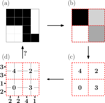
More specifically, the results of the present paper are motivated by the task of enhancing the resolution of reconstructed tomographic images obtained from binary objects representing, for instance, crystalline structures, nanoparticles or two-phase samples [1, 3, 7, 46, 49]. The reconstructed tomographic image might contain several gray levels, which, depending on the accuracy of the reconstruction, result from the fact that low-resolution pixels may cover different numbers of black high-resolution pixels. For turning the grayscale image into a high-resolution binary image we utilize the gray levels and two additional high-resolution projections, which may have been acquired by different imaging techniques or modalities (e.g., via scanning transmission electron microscopy [46]). More precisely, we study the task of reconstructing binary -images from row and column sums and additional constraints, so-called block constraints, on the number of black pixels to be contained in the -blocks resulting from a subdivision of each pixel in the low-resolution image. We remark that we do not require that the X-ray data are taken from orthogonal directions. In our context it suffices that the X-ray data have been taken with high-resolution according to the discretization of the low-resolution image.
Figure 1 illustrates the process. The example given in this figure also shows that the block-constraints can help to narrow down the solution space. In fact, the solution shown in this figure is uniquely determined by the input (the row and column sums and block constraints). The row and column sums alone do not determine the solution uniquely and, of course, neither do the block constraints.
Apart from super-resolution imaging [29, 33, 35, 37, 42, 47], and its particular applications [8, 20, 40, 48] in discrete tomography [1, 17, 22, 25, 26, 28, 30, 32, 45], the problems discussed in this paper are also relevant in other contexts.
From a combinatorial point of view, they can be viewed as reconstructing binary matrices from given row and column sums and some additional constraints. Unexpected complexity jumps based on the results of the present paper are discussed in [6] and, to some extent, at the end of this section. Background information on such problems involving different kinds of additional constraints can be found in [11, Sect. 4].
Other applications belong to the realm of dynamic discrete tomography [5, 6, 7, 49]. For instance, in plasma particle tracking, some particles are reconstructed at time Between and the next time step the particles may have moved to other positions. The task is to reconstruct their new positions, again from few projections. One way of incorporating additional prior knowledge about the movement leads to block constraints of the kind discussed in this paper; see [5].
As the task of reconstructing a binary matrix from its row and column sums can be formulated as the task of finding a -matching in a bipartite graph, we remark that our theorems can also be seen as results on finding -matchings that are subject to specific additional constraints. Related (but intrinsically quite different) results on matchings subject to so-called budget constraints can be found, e.g., in [21].
For super-resolution imaging the two main contributions of this paper are as follows. On the one hand, we show that reliable bimodal tomographic data can be utilized efficiently, i.e., the resolution, in each dimension, can be doubled in polynomial time if the gray levels of the low-resolution image have been determined precisely (Thm. 1). On the other hand, the task becomes already intractable (unless ) if the gray levels of some pixels come with some small error of (Thm. 3 and Cor. 2). This proves that noise does not only affect the quality of the reconstructed image but also the algorithmic tractability of the inverse problem itself. Hence the possibility of compensating noisy imaging by including bimodal information may in practice be jeopardized by its algorithmic complexity. While this is not the focus of the present paper let us point out that, even in the presence of (a reasonably restricted degree of) noise, the approach leading to Thm. 1 can, in principle, be extended to a fast heuristic for doubling the resolution of such images in each dimension. At present, however, we do not know how such an approach would compare with other heuristics on real-world data.
From the perspective of discrete tomography, the contributions of this paper can be interpreted as follows. It is well known that the problem of reconstructing binary images from X-ray data taken from two directions can be solved in polynomial time [16, 41]. Typically, this information does not determine the image uniquely (see, e.g., [23] and the papers quoted there). Hence, one would like to take and utilize additional measurements. If, however, we add additional constraints that enforce that the solutions satisfy the X-ray data taken from a third direction, then the problem becomes -hard, and it remains -hard if X-ray data from even more directions are given [18] (see also [15] for results on a polyatomic version).
As it turns out, the case of block constraints behaves somewhat differently. Thm. 3 and Cor. 2 show that the problem of reconstructing a binary image from X-ray data taken from two directions is again -hard if we add several (but not all) block constraints (which need to be satisfied with equality). However, and possibly less expectedly, if we include all block constraints, then the problem becomes polynomial-time solvable (Thm. 1). If, on the other hand, from all block constraints some of the data come with noise at most then the problem becomes again -hard (Thm. 3 and Cor. 2). And yet again, if from all block constraints all of the data are sufficiently noisy, then the problem is in (as this is again the problem of reconstructing binary images from X-ray data taken from two directions). An overview of these complexity jumps is given in Fig. 2.

2. Notation and Main Results
Let and denote the set of integers, natural numbers, and non-negative integers, respectively. For set and With 11 we denote the all-ones vector of the corresponding dimension. The cardinality of a finite set is denoted by
In this paper we use Cartesian coordinates (rather than matrix notation) to represent pixels in an image. In particular, the two numbers and in a pair denote the - and -coordinate of a point, respectively. In the following we consider grids The set and is called column and row respectively. Let, in the following, Any set is a vertical strip (of width ). A horizontal strip (of width ) is a set of the form
Sets of the form with and are called boxes. For let Defining for any and the set of (lower-left) corner points we call any box with a block. The blocks form a partition of i.e.,
Let us remark that, as defined, all our images consist of lattice points. However, the figures will be given in terms of pixels. Accordingly, the block will be depicted as see Fig. 3. The individual pixels are i.e., are identified with the lattice point at their lower left corner. Of course, the fact that a point is or is not present in a solution is indicated by a black or a white pixel, respectively.

For with we define the task of (noisy) super-resolution
nSR
| Instance: | |||||||
| (row sum measurements) | |||||||
| (column sum measurem.) | |||||||
| (corner points of reliable | |||||||
| gray value measurem.) | |||||||
| (gray value measurem.) | |||||||
| Task: | Find with | ||||||
| (row sums) | |||||||
| (column sums) | |||||||
| (block constraints) | |||||||
| (noisy block constraints) | |||||||
| or decide that no such solution exists. | |||||||
The numbers and are the row and column sum measurements of the high-resolution binary image, corresponds to the gray value of the low-resolution -pixel at of the low-resolution grayscale image, and is the set of low-resolution pixel locations for which we assume that the gray values have been determined reliably, i.e., without error. The number is an error bound for the remaining blocks. (While it may seem unusual to denote a non-negative integer by we chose this notation to indicate the specific role of of quantifying an error.) The task is to find a binary high-resolution image satisfying the row and column sums such that the number of black pixels in each block is the gray value for the corresponding -pixel low-resolution image. Clearly, a necessary (and easily verified) condition for feasibility is that
In the following we will assume without loss of generality that this is always the case.
Our special focus is on double-resolution imaging, i.e., on the case For we define nDRnSR In the reliable situation, i.e., for we simply speak of double-resolution and set DRnSR (Then, of course, the set can be omitted from the input.)
In the present paper, we show that the resolution of any reliable grayscale image can in fact be doubled in each dimension in polynomial-time if X-ray data are provided from two viewing angles at double-resolution. In other words, we show
Theorem 1.
Figures 4 and 5 illustrate the performance of the algorithm for DR applied to two phantoms. The results have been obtained within a fraction of a second on a standard PC.
In Fig. 4, the original phantom is a binary image of a crystalline sample taken from [2]. It is assumed that the low-resolution grayscale image shown in Fig. 4(a) has been obtained by some imaging method and that double-resolution X-ray information in the two standard directions is also available. Application of the algorithm (see Algorithm 1) yields the binary image shown in Fig. 4(c).
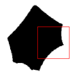


In Fig. 5, the original phantom is a binary image, for which the low-resolution grayscale image shown in Fig. 5(a) is available. From this image and the row and column sums (counting the black pixels) of the original phantom the algorithm returns the binary image shown in Fig. 5(b).


The results shown in Figs. 4 and 5 satisfy, of course, the row and column sums and block constraints. However, in both cases the solutions are still not unique. This can also be detected in polynomial time.
Theorem 2.
For every instance of DR it can be decided in polynomial time whether the instance admits a unique solution.
While the additional X-ray information (at double-resolution) does in general reduce the ambiguity, typically it will still not lead to uniqueness. Of course, a standard way of dealing with non-uniqueness in practice is regularization [8, 9, 24, 38]. To illustrate the possibility of adapting a regularization scheme to our context, we show in Fig. 5(c) a binary solution minimizing the total variation (TV). In fact, the solution is obtained from Fig. 5(a) by applying so-called local switches, each of which is strictly decreasing the value of the total variation functional
where
and denotes the Euclidean norm. See, e.g., [12] for some background information. Of course, we obtain the same results for other -norms (including the -norm), because our images are binary.
We now turn to the task where small “occasional” uncertainties in the gray levels are allowed. First observe that a constant number of uncertainties does not increase the complexity. However, if we allow a (as we will see, comparably small but) non-constant number of uncertainties the problem becomes hard.
Theorem 3.
nDR is -hard for any
(For background material on complexity theory, see, e.g., [19].)
Further, the -hardness extends to the task of checking uniqueness.
Corollary 1.
The problem of deciding whether a given solution of an instance of nDR with has a non-unique solution is -complete.
As it turns out, the problem nDR with remains -hard for larger block sizes.
Corollary 2.
nSR is -hard for any and
In other words, noise does not only affect the reconstruction quality. It also affects the algorithmic tractability of the inverse problem.
3. Reliable Data
In this section we discuss the task DR, i.e., and We remark that, in the following, our emphasis is on providing brief and concise arguments for polynomial-time solvability rather than to focus on computationally or practically most efficient algorithms. Recall, however, our comments on the computational performance of our algorithms and the effect of the additional information for the example images depicted in Figs. 4 and 5.
The main result of this section is Thm. 1. In its proof we show that DR decomposes into five problems that can be solved independently. The five problems are restricted single-graylevel versions of DR where each block is required to contain the same number of ones. In fact, we allow for restricted problem instances (and in particular row and column sums) to be defined only on subsets
| (3.1) |
of the grid given by means of some Let
and
denote the projection of onto the first and second coordinate, respectively.
Then, we define for
DR
| Instance: | ||||||||
| (a set of corner points) | ||||||||
| (row sum measurem.) | ||||||||
| (column sum measurem.) | ||||||||
| Task: | Find with | |||||||
| (row sums) | ||||||||
| (column sums) | ||||||||
| (block constraints) | ||||||||
| or decide that no such solution exists. | ||||||||
Of course, the tasks DR are trivial. In fact, the only potential solution satisfying the block constraints is given by and it is checked easily and in polynomial time whether this satisfies the row and column sums.
The next lemma and corollary deal with , Their statements and proofs use the notation and for the number of blocks in the same vertical strip as but below or in the same horizontal strip as but left of respectively. More precisely, let
for
Lemma 1.
-
(i)
An instance of DR is feasible if, and only if, for every we have
-
(ii)
The solution of a feasible instance of DR is unique if, and only if, for every we have
-
(iii)
DR
Proof.
Clearly, for the feasibility of a given instance of DR the conditions
are necessary.
Now, suppose that the conditions are satisfied. For every and we set
| (3.2) | ||||
Figure 6 gives an illustration.

By this definition we have satisfied all block constraints. A simple counting argument shows that the row and columns sums are also as required. In fact, for and we have
This concludes the proof of (i).
To show (ii), we consider a solution to Suppose that and for some Then, there exist with By the block constraints we have Applying a switch to and i.e., setting and otherwise, yields thus another solution. As the same argument holds also for the column sums we have shown that the condition in (ii) is necessary. The condition is, on the other hand, also sufficient since the 0-values of the row and column sums leave only a single position in each block for which can take on a non-zero value (in fact, the value needs to be 1 to satisfy the block constraints).
Corollary 3.
-
(i)
An instance of DR is feasible if, and only if, for every we have
-
(ii)
The solution of a feasible instance of DR is unique if, and only if, for every we have
-
(iii)
DR
Proof.
The results follow directly from the results for in Lem. 1 as the former are obtained from the latter by inversion and vice versa, i.e., by replacing by and by and, in the solutions, all ’s by ’s and ’s by ’s. ∎
Next we prove polynomial-time solvability of To this end we need two lemmas. The first can be viewed as dealing with a certain “two-color version” of discrete tomography. The second deals with specific switches or interchanges (in the sense of [41]).
Lemma 2.
The problem, given and decide whether there exist non-negative integers such that
and, if so, determine a solution, can be solved in polynomial time.
Proof.
We show that the problem can be formulated as a linear program involving a totally unimodular coefficient matrix (for background material, see [44]).
We assemble the variables for into a -dimensional vector and rephrase the constraints in matrix form and where contains the ’s, contains the ’s, and denotes the -identity matrix. The problem is then to determine an integer solution of where
The submatrix
is totally unimodular as it is the node-edge incidence matrix of a bipartite graph (one of the two parts of the partition is the set of the last rows of ). But then is also totally unimodular as it results from appending a subset of rows of to the totally unimodular matrix In other words, is an integral polyhedron, i.e., it coincides with the convex hull of its integral vectors. Hence, a vertex of this polyhedron can be found in polynomial time by linear programming. ∎
Next we study the structure of solutions in terms of the patterns of the blocks. This will allow us to focus on special classes of solutions, which we will later call reduced solutions. The problem of finding reduced solutions to a given instance of DR will decompose into the five independent subtasks of solving instances of The concept of reduced solutions will also play a role in our proof of Lem. 4 showing that
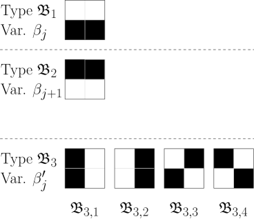
Blocks in solutions are filled with zeros and ones. There are 16 such combinations. By grouping the combinations that have the same row sums, we distinguish the nine block types shown in Fig. 7. Some of the types consist of several subtypes/combinations: type and consist of the two subtypes and respectively, while consists of the subtypes . For any given solution, we will later count the number of occurrences of the different block types in each horizontal and vertical strip. The corresponding variables for the horizontal strip are indicated in Fig. 7. For instance, counts the number of occurrences of block type while counts the number of occurrences of block type
We introduce now the concept of local switches. It is based on the following observation. If, for instance, a horizontal strip contains a block of type and another one of type we may replace them by a block of type and a block of type respectively, without changing the row and column constraints. Such a change will be called a horizontal local switch of class In a similar way we define horizontal local switches of class according to Table 1. Horizontal local switches of class affect only single blocks (blocks of type are turned into blocks of type ).
The (similar) switches in the vertical strips, called vertical local switches, are listed in Table 2.
| Class | Turns | Into | Illustration | ||
|---|---|---|---|---|---|
![[Uncaptioned image]](/html/1701.04399/assets/x15.png)
|
|||||
![[Uncaptioned image]](/html/1701.04399/assets/x16.png)
|
|||||
![[Uncaptioned image]](/html/1701.04399/assets/x17.png)
|
|||||
![[Uncaptioned image]](/html/1701.04399/assets/x18.png)
|
|||||
![[Uncaptioned image]](/html/1701.04399/assets/x19.png)
|
|||||
![[Uncaptioned image]](/html/1701.04399/assets/x20.png)
|
|||||
![[Uncaptioned image]](/html/1701.04399/assets/x21.png)
|
| Class | Turns | Into | Illustration | |
|---|---|---|---|---|
![[Uncaptioned image]](/html/1701.04399/assets/x22.png)
|
||||
![[Uncaptioned image]](/html/1701.04399/assets/x23.png)
|
||||
![[Uncaptioned image]](/html/1701.04399/assets/x24.png)
|
||||
![[Uncaptioned image]](/html/1701.04399/assets/x25.png)
|
||||
![[Uncaptioned image]](/html/1701.04399/assets/x26.png)
|
||||
![[Uncaptioned image]](/html/1701.04399/assets/x27.png)
|
||||
![[Uncaptioned image]](/html/1701.04399/assets/x28.png)
|
A switch is called local if it is a horizontal or vertical local switch of some class A solution is called reduced if no local switch of any class can be applied. Note that local switches are directed in the sense that they turn the types of blocks listed in the second column of Tables 1 and 2 into the types given in the respective third column of the tables. Oppositely directed switches, called reversed local switches, will be used later when we discuss questions of uniqueness.
Lemma 3.
-
(i)
Application of a local switch to a solution of a given instance of DR yields again a solution of the same instance.
-
(ii)
An instance of DR has a solution if, and only if, there is a reduced solution.
Proof.
To prove (i) just observe that the local switches do neither change the row and column sums nor the number of ones contained in each block.
Let us now turn to (ii). Suppose the given instance has a solution The local switches of class increase the number of blocks of type i.e.,
The process of applying local switches of class thus needs to terminate since the number of blocks in each problem instance is finite. Further, note that local switches of class applied in horizontal strips increase the number of blocks of type The vertical switches of that class do not decrease the number of such blocks, but increase the number of blocks which are of type or Hence, after finitely many switches, a given solution is converted into a reduced one. ∎
Lemma 4.
Proof.
Our general strategy is as follows. First we show that a given instance is feasible if, and only if, there exists a specific reduced solution that contains only three block types. Then we give a polynomial-time algorithm that finds such a solution or determines infeasibility.
By rearranging the rows and columns, if necessary, we may assume that
Now, first suppose that the given instance has a solution. Then, by Lem. 3 there exists a reduced one. In the following, we consider such a reduced solution.
The potential block types, and corresponding variables and counting the number of occurrences of the respective block types in the horizontal strip of a reduced solution, are shown in Fig. 7(b). Block types counted by the same variable have equal row sums.
Consider now for fixed the blocks in Counting the block types, any solution needs to satisfy
which implies
| (3.3) |
As the solution is reduced no horizontal local switch of class can be applied, hence it is impossible that both and This, together with and (3.3), implies
(Note that by there is no block of type As no horizontal local switch of class can be applied, there is neither a block of type .)
The same argument applies to the other horizontal strips, and a similar argument holds for the vertical strips (which, in particular, rules out blocks of type ). Hence, we conclude that, due to reduction, amounts to the task of assigning one of the three block types shown in Fig. 8 to each of the blocks such that, in particular, the number of type and type blocks in each horizontal and vertical strip, respectively, equals some prescribed cardinality.

Now, we introduce -variables that are one if, and only if, is of type respectively. Then we ask for -solutions that satisfy
Eliminating we see that the -solutions of this system are in one-to-one correspondence with the solution of
| (3.4) |
As we assume that our instance is feasible (hence containing two ones in each block), we have and for every and Hence, if a solution to (3.4) is expanded, replacing the by the respective block types, then, indeed
for every and Any -solution to (3.4) provides thus a solution to the given instance. Since -solutions to (3.4) can be found in polynomial time (see Lem. 2), we have hence determined a solution to our instance in polynomial time. Note that this solution is reduced as it does not contain blocks of type and
Let us now turn to the task of solving DR. Suppose, we are given a feasible instance of DR that does not contain any block constraints of the form and whose row and column sums satisfy
| (3.5) |
We call such an instance a proper instance.
In the following, we consider for fixed the horizontal strip . We set
Let us now consider a solution of the proper instance. A count of the block types of the solution in that strip (the variables for the block types are indicated in Fig. 7), yields
| (3.6) | |||||||||||||||||
| (3.7) | |||||||||||||||||
| (3.8) | |||||||||||||||||
From the system we obtain
| (3.9) | |||||||||||||
| (3.10) |
We will show that for reduced solutions, the variable values of are uniquely determined and can, actually, be computed from the data (i.e., from and ). This will then allow us to split the task into instances of
We begin with a simple observation.
Lemma 5.
Any reduced solution to a proper instance of DR satisfies
Proof.
Given a proper instance, we distinguish three cases.
-
•
Case 1: Every reduced solution satisfies
-
•
Case 2: There is a reduced solution satisfying and in any such solution we have
-
•
Case 3: There is a reduced solution satisfying
Lemma 6.
Given a proper instance of DR. Then,
| Case 1 | |||||||||
| Case 2 | |||||||||
| Case 3 |
and in all cases the variable values of are uniquely determined by the data.
Proof.
By Lem. 3, a proper instance has a reduced solution. Hence, one of the disjoint Cases occurs. Once we have established the implications “” the reverse implications follow, because the stated intervals for the are disjoint (thereby uniquely specifying the case).
Hence it suffices to prove the implications “.” Let us begin with Case 1. As we cannot apply any further horizontal local switch of class we must have hence and Eq. (3.10) implies As we thus have Further, (3.7) yields Hence, all values of the variables are uniquely determined.
We are now prepared to give a proof of Thm. 1.
Proof of Thm. 1.
We show that the task of finding a solution to a given problem instance can be decomposed into five independent subtasks of solving instances of The subtasks are then polynomial time solvable by Lem. 1, Cor. 3 and 4 (and trivially for and ). The key step in our proof is to deduce from the data the row and column sums for the particular subtasks. This deduction is possible for reduced solutions.
We start with some preprocessing if necessary. First, if the problem instance contains block constraints of the form we need to have In this case, we fix the values of these variables, reduce the row and column sums accordingly, and consider only the remaining blocks. For notational convenience, we assume from now on that our instance does not contain such block constraints.
Second, by possibly rearranging the rows and columns, we assume that (3.5) holds.
Suppose, the problem instance is feasible, hence proper. (We return to the infeasible case later.) The instance has a solution and, hence by Lem. 3, a reduced one. Thus, considering a horizontal strip with one of the Cases 1, 2 or 3 needs to occur. Which of the cases occurs is, by Lem. 6, determined by the data, simply by testing whether we have
| or | (3.11) | ||||||||||||
| or | |||||||||||||
In all three cases we know the unique values of the and Therefore we know for each the row sums
with
for according to (3.1). In particular, we have
| (3.12) |
Similarly, we obtain the individual vertical constraints. We can therefore decompose the reconstruction problem into the three independent subproblems which, by Lem. 1, Cor. 3, and Lem. 4, are solvable in polynomial time.
It remains to consider the case that the given instance of DR is infeasible. In this case, the decomposition into the subproblems needs to yield either an infeasible subproblem or the returned “solution” needs to violate one of the constraints. As both are detected in polynomial time, we have concluded the proof of this theorem. ∎
Note that the above proof is constructive. A corresponding polynomial-time algorithm for solving DR is summarized in Algorithm 1.
We also remark that the solutions returned by the proposed algorithm are always reduced. This is easily seen by (i) verifying that the values and in each of the three cases in (3.11) (and correspondingly for the variables in the vertical strips) do not allow an application of any of the local switches of class because for each of the local switches there is always a corresponding variable of value zero; and (ii) by noting that the proposed algorithm for returns, by definition, only solutions where no local switch of class can be applied.
Now we turn to uniqueness.
Proof of Thm. 2.
By Thm. 1, either infeasibility is detected or a reduced solution of an instance is determined in polynomial time. We can thus assume that the problem instance has a solution.
Clearly, a solution is unique if, and only if (Condition 1:) there is only one reduced solution, and (Condition 2:) every solution is a reduced solution.
The solution returned by the algorithm is reduced. Any two reduced solutions define the same instances of the subproblems because the problem instances are defined by means of (3.11), i.e., the definition depends only on the particular values of the and (note that can be directly determined from the input). Hence, there is only one reduced solution if, and only if, the solution to each of the subproblems is unique.
The conditions in Lem. 1(ii) and Cor. 3(ii), and hence uniqueness for the instances of and can be checked in polynomial time. For we have by the linear program considered in Lem. 2, a basic feasible solution of the linear program, i.e., a vertex of the feasible region, at our disposal. Now we minimize the linear objective function over the same feasible region, which again can be done in polynomial time. The solution is unique if, and only if, (Note that multiple solutions contain the same number of ones as this is given by the sum of the row and column sums, respectively.) Hence uniqueness for , and therefore Condition 1, can be checked in polynomial time.
Suppose now that the reduced solution returned by the algorithm is unique among all reduced solutions, i.e., Condition 1 is satisfied. We have shown in Lem. 3 that every solution can be reduced by applying a sequence of local switches. Reversing the sequence and the local switches, we thus see that Condition 2 holds if, and only if, there is no reversed local switch that can be applied to There are possible pairs of blocks that need to be checked to form a reversed local switch, hence Condition 2 can also be checked in polynomial time. ∎
4. Data Uncertainty
1-In-3-SAT
Instance:
Positive integers and a set of clauses over variables where each clause consists of three literals involving three different variables.
Task:
Decide whether there exists a satisfying truth assignment for that sets exactly one literal true in each clause.
For a given instance of 1-In-3-SAT we will construct a circuit board that contains an initializer, several connectors, and clause chips. A truth assignment is transmitted through the circuit board, the clause chips ensure that the clauses are satisfied.
The structure of our proof is in some ways similar to the proof from [18] that establishes the -hardness of the task of reconstructing lattice sets from X-rays taken in three or more directions. However, we need to deviate from [18] in several key aspects, because the block constraints do not give a direct way of controlling points over large distances, and the elimination of “unwanted solutions” inside individual blocks seems also problematic. A fundamental difference to [18] is, for instance, that we encode the Boolean values for the variables by specific types of blocks, and the satisfiability of the clauses is verified via row and column sums. At first glance it seems that part of the variable assignment information is lost after verification, but it turns out that we can recover it from “redundant” information in our encoding.
Key ideas of the proof of Thm. 3. Before we start with the detailed proof, we illustrate the general ideas by means of an example. Suppose, the instance of 1-In-3-SAT is given by We will define an instance of nDR such that there is a solution for if, and only if, there is one for To this end, we construct a circuit board contained in the box With each we associate a variable Again, the figures will show the associated pixels see Fig. 3.
The circuit board consists of three major types of components: An initializer, connectors, and clause chips. The initializer and the connectors are rather similar. The initializer contains for every variable a so-called -chip, the connectors contain for every variable a -chip. The clause chips are more complex as they consist of two collectors, two verifiers, and a transmitter.
Figure 9(a) shows the circuit board for our instance.
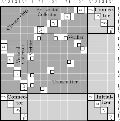
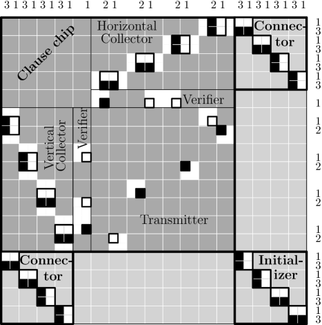
The gray areas indicate blocks that are set to zero via block constraints. By setting to zero suitable row and column sums we make sure that non-zero components are only possible in the white bold-framed boxes. The non-zero row and column sums are shown on the top and on the right of the figure.
The bold-framed boxes are Boolean chips, which are, according to their position on the circuit board, further classified into and -chips, In these chips we will encode the respective Boolean values for the variables and , All blocks, except for those set to zero, are allowed to contain at most two ones. The blocks containing the -chips are required to contain precisely two ones.
In each clause chip there are two strips playing a special role. One is a horizontal strip containing a so-called horizontal verifier, the other is a vertical strip containing a so-called vertical verifier (see rows 25 and 26, and columns 9 and 10 in Fig. 9(a)). A key property of our construction is that the truth assignments will be in 1-to-1 correspondence with the solutions of the constructed nDR instance if the row and column sum constraints related to the verifiers are left unspecified. The row and column sum constraints related to the verifiers will then ensure that the truth assignments are in fact satisfying truth assignments.
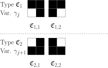
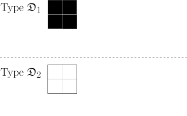
We can already begin to see how a truth assignment for our particular instance will provide a solution for Utilizing the type 1 and type 2 blocks shown in Fig. 10, we set each -chip, of the initializer to type 1 if otherwise we set it to type 2.

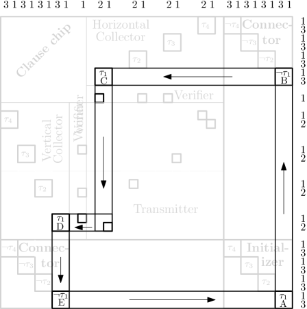
Let us, as an example, consider and the sequence of Boolean chips marked A, B, C, D, and E in Fig. 9(a); see also Fig. 11. The chips A and B lie in the same vertical strip, and since A is of type 1, B needs to be of type 2 in order to satisfy the column sums in the vertical strip. Chip C must be of type 1 to satisfy the row sums in the horizontal strip. Then, the remaining points in the two vertical strips intersecting chip C are uniquely determined by the column sums. In particular, the point of the transmitter in a row intersecting D must be 0. Now, chip D needs to contain two ones since the vertical strip containing chip D contains four ones, two of which need to be contained in chip E via block constraints. Hence, we conclude from the row sums that D is of type 1. Considering now the vertical strip intersecting D we see that chip E is of type 2, and therefore, together with chip A, satisfies the row sums in the horizontal strip. Thus, the -chips are consistently of type 1, and the -chips are of type 2. Note that we have satisfied all row and column sums for the strips intersecting one of the chips A,B,C,D, and E. Moreover, the block constraints in these chips are also satisfied.
Turning to the Boolean chips for we conclude with a similar reasoning that the - and -chips are consistently of type 1 and type 2, respectively. We have now satisfied the block constraints for the - and -chips, Additionally, we satisfied the row and column sums for the strips intersecting one of these chips. Clearly, we have not violated any of the previously satisfied constraints as there is no row or column that intersects both a Boolean chip for and
We say that we have deduced the types of the Boolean chips for by vertical transmission, because in our previous chain of arguments we started by considering the vertical strip containing the respective Boolean chip of the initializer (see also Fig. 11).
Note that such a vertical transmission does not directly work for the assignment False of the variables since the column sums do not allow us to deduce a unique solution for the respective -chip. Hence for the Boolean chips for we resort to horizontal transmission to deduce the types of the respective - and -chips. In this way we conclude that the - and -chips are consistently type 2 and type 1, respectively.
Figure 9(b) shows the solution that we obtain by the previous arguments. All constraints, in particular also the row and column sums in the verifiers, are satisfied. We will later see in general that there is a single one in each of the two verifiers of the -clause chip, if, and only if, exactly one of the three literals appearing in the -th clause is True.
Now, consider the reverse direction for the proof, i.e., suppose a solution to our instance of Fig. 9(a) is given. Note that if we can ensure that the types of the Boolean chips in the initializer are either 1 or 2 then by the previous arguments we have a satisfying truth assignment for by setting if, and only if, the corresponding -chip of the initializer is of type 1.
The respective block, row and column sum constraints allow only the four possible types of blocks for the Boolean chips of the initializer shown in Fig. 10. The types 3 and 4, however, are ruled out by the following “global” argument: Suppose, for some the -chip of the initializer is of type By horizontal transmission, we then conclude that the -chips need to be of type 1 (by transmitting, as before in a unique way, through each clause chip). By vertical transmission, however, we conclude that the -chips are of type 2, which is a contradiction.
We remark that effectively we utilize the noisy block constraints at three different places in our construction. They are needed, because we can neither prescribe the exact number of ones in the -chips of the horizontal or the vertical collectors, nor in the -configurations that are introduced later and which involve the transmitters (see also Figs. 13, 15, and 14).
Having illustrated the key ideas behind the construction, we now turn to the formal proof.
Proof of Thm. 3.
Let in the following denote an instance of 1-In-3-SAT. We will define an instance of nDR such that there is a solution for if, and only if, there is one for The circuit board will be contained in the box
With each we associate a variable Figure 12 illustrates the general layout of the construction.
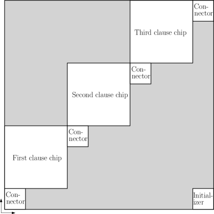
We define the instance of nDR by specifying the row sums the column sums and the block constraints. For notational convenience we define the block constraints via a function In this notation, denotes the block constraint
while signifies the block constraint
The set of reliable block constraints for is then
The different components of the circuit board are placed at specific positions. For a more compact definition of these positions we set
Turning to the definition of the initializer, we remark that the initializer is contained inside the box We will specify the row and column sums when the corresponding connectors are introduced. In terms of the block constraints we define for every
The block will be called -chip (of the initializer). For an illustration of an initializer, see the bottom right -box in Fig. 9(a).
We define connectors. Each connector is contained inside a box with In terms of block constrains we define for every and
For the row and column sums we define for every and
The block will be called -chip (of the -th connector). For an illustration of a connector, see the bottom left -box in Fig. 9(a).
Next we define the clause chips. Each clause chip is contained in a box with The box is a (vertical) collector, the box is a (vertical) verifier, the box is a transmitter, the box is a (horizontal) verifier, and the box is a (horizontal) collector. For an illustration of a clause chip, see the top left -box in Fig. 9(a) depicted in dark gray.
For we define the row sums of the horizontal and the column sums of the vertical verifiers (we will call these row and column sums verifier sums) by
The remaining row and columns sums for the transmitters (meeting also certain verifiers and collectors) are for and defined by
Note that sums for the rows and columns meeting the collectors are already defined as there is a transmitter or connector for each row and column meeting a collector (see also Fig. 12). We have thus completed our definition of the row and column sums of our instance and continue now with the remaining block constraints.
For the vertical collector, we define for every and
The box will be called -chip (of the -th vertical collector).
Similarly, for the horizontal collector we define for every
The box will be called -chip (of the -th horizontal collector).
Note that the -chips, of the collectors are not contained in blocks. In fact, each such -chip intersects two blocks (which, in turn, are allowed to contain at most two ones). For any we will also refer to the - and -chips on the circuit board as Boolean chips.
For the empty space above the vertical collector, i.e., for and we define
Now we turn to the block constraints for the clause-dependent part of chip, i.e., the verifiers and the transmitters.
With and we denote the indices of the variables that appear unnegated and, respectively, negated in the -th clause. For instance, for (regarded as the first clause) we have and
Depending on whether a given variable appears negated, unnegated or not at all in the -th clause, we will distinguish three different types of verifier and transmission parts forming a so-called -configuration. Formally, for and we refer to the sets of points
as -configuration. Figure 13 gives an illustration.
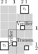
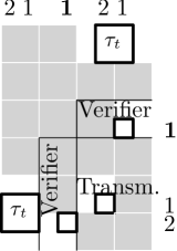
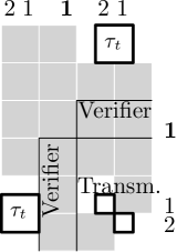
For the three different types of -configurations, we need to set different blocks to zero. The formal definition is as follows.
For the vertical verifiers we define for every and
Similarly, for the horizontal verifiers we define for every and
For the transmitters we define for every and
The remaining block constraints in the transmitter are set to zero, i.e., for every with we set
Outside the initializer, connectors, and clause chips we set everything to zero, i.e., for every with
| (4.1) |
we set
This concludes the formal definition of the instance We shall now show that admits a solution if, and only if, the 1-In-3-SAT instance admits a solution.
Let denote the set of points of the Boolean chips and -configurations,
Claim 1: In any solution of we have for every
To see this, we first remark that the claim holds for all points outside each clause chip since the only blocks there that are not set to zero are the Boolean chips of the initializer and connectors. For the points inside a clause chip, we need to distinguish three cases since there are three differently structured -configurations, in which different blocks are set to zero. They are shown in Fig. 13. In all three cases the points outside the corresponding Boolean chips in the two collectors and the -configuration are either set to zero by block constraints or by zeros of suitable row or column sums. This shows the claim.
Claim 2: In any solution of every - and -chip, is of one of the types from shown in Fig. 10.
For this, consider a fixed index Each -chip is contained in a horizontal or vertical strip that, except for a -chip, contains no other points of Since by the block constraints each -chip contains two ones, and since the respective row or column sums in the strip sum up to four there need to be exactly two ones also in each -chip. The row and column sums enforce that no two ones are in the rightmost column and upper row of the box of each -chip. Hence, there are at most the four possibilities shown in Fig. 10.
Claim 3: In any solution of all the -chips (for a given ) are either of type 1 or type 2.
To show this, consider again a fixed index Let denote the sequence with (i) is the -chip of the initializer, (ii) is the -chip of the -th connector, (iii) is the -chip of the -th connector, (iv) is the -chip of the -th horizontal collector, (v) is the set of points in the transmitter of the -configuration of the -th clause, and (vi) is the -chip of the -th vertical collector, see Fig. 11 for the case and Fig. 12 again for the general layout.
By horizontal transmission (see Fig. 14) and Claim 2, we have the following implication: If a -chip of is of type 2, 3 or then the -chip of is of type 2, and the points of are also uniquely determined.
By vertical transmission (see Fig. 15) and Claim 2, we have the following implication: If a -chip of is of type 1, 3 or then the -chip of is of type 1, and the points of are also uniquely determined.


Hence, if we start at an arbitrary -chip and perform vertical and horizontal transmissions that meet at some Boolean chip we obtain a contradiction unless the -chip was of type 1 or 2.
The types 1 and 2 can be associated with Boolean values. In -chips, and in particular those of the initializer, we associate with type 1 the value True and with type 2 the value False.
Claim 4: There is a 1-to-1 correspondence between the (not-necessarily satisfying) truth-assignments for and the solutions to the -variant of that allows violation of the verifier sums, i.e., of the column sum constraints for the vertical verifiers or the row sum constraints for the horizontal verifiers.
By construction, there is neither a horizontal nor a vertical strip that intersects the Boolean chips for two variables with The arguments from Claim 3 are thus independently valid for each We can hence consider an arbitrary (not-necessarily satisfying) truth-assignment for fill in the corresponding types in the initializer and extend them to yield a solution to the -variant of with unspecified verifier sums. Vice versa, the chip types in the initializer of a solution to yield a truth-assignment for We have already seen in the proof of Claim 3 that the type of each -chip, in the initializer determines all ones in the corresponding -chips and -configurations, Hence, the correspondence is indeed 1-to-1.
Claim 5: The satisfying truth-assignments of are in 1-to-1 correspondence with the solutions of
This can now be seen by observing that the -chip, of the -th horizontal and vertical collector, contributes a one to the horizontal and also to the vertical verifier in the -th clause chip if, and only if, the -chip is True (is of type 1) with or the -chip is False (is of type 2) with ; see Figs. 13, 15(a,b,c), and 14(a,b,c). The verifier sums thus ensure that exactly one literal in the -th clause is True. This, together with Claim 4, proves the claim.
By Claim 5, admits a solution if, and only if, admits a solution.
Finally, we note that the transformation runs in polynomial time. ∎
In section 2 we remarked that can be viewed as version of DR where small “occasional” uncertainties in the gray levels are allowed. Reviewing the proof of Thm. 3, the term “occasional” can be quantified as meaning “of the order of the square root of the number of blocks.” More precisely, of blocks on the circuit board, there are with uncertainty.
Let us further remark that the arguments in the above proof do not rely on the particular value of in the noisy block constraints. These constraints can be replaced by any other types of block constraints, certainly as long as they allow for 0, 1, and 2 ones to be contained in each of the corresponding blocks. By this observation it is possible to adapt our proof to several other contexts where the reconstruction task involves other types or combinations of block constraints; see [6].
Finally, note that the transformation in the proof of Thm. 3 is parsimonious (see Claim 5 in the above proof). Hence the problem of deciding whether a given solution of an instance of nDR with has a non-unique solution is -complete (which proves Cor. 1); for an -hardness proof of Unique-1-in-3-SAT see [18, Lem. 4.2].
Proof of Cor. 2.
We use a transformation from nDR Let
denote an instance of nDR Note that and are even.
We set and For and we define
and
This gives the instance
of nSR Clearly, the instance of nDR admits a solution if, and only if, the instance of nSR admits a solution (by filling/extracting the -blocks of into/from the -blocks of ). This is a polynomial-time transformation, proving the corollary. ∎
5. Final Remarks
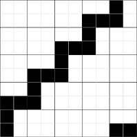
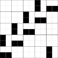
Recall that in the proof of Thm. 1 we have made extensive use of the concept of local switches. Each such switch involves four points. Figure 16 shows, on the other hand, two solutions of a DR instance that differ by -pixels. It is easily checked that these are the only solutions for the given instance (Note that we used such a structure in the proof of Thm. 3). Hence, there is no sequence of small switches transforming one solution into the other. The existence of such large irreducible switches is well-known for the -hard reconstruction problem from more than two directions [31] (and would follow independently from ). The problem however, admits large switches albeit is polynomial-time solvable.
In addition to the block constraints our computational tasks rely only on row and column sums, i.e., projection data from two viewing angles. For more than two viewing directions we obtain the -hardness of nSR for any and directly from the construction in [18]. The -hardness of the corresponding variants of nSR for can also be derived from [18]. First the construction is thinned out so as to make sure that each block contains at most one element of the grid of candidate points. Then, a second copy with inverted colors is interwoven by applying a translation by or This ensures that each non-empty block contains exactly one one.
The complexity status of nSR remains open for We conjecture that the problem is -hard for larger
Also, it would be interesting to analyze the effect of the results of the present paper on the “degree of ill-posedness” of the underlying problem (see [4]).
Acknowledgments
We are grateful to the anonymous referees for their valuable comments on a previous version of the paper. This work was supported by the German Research Foundation Grant GR 993/10-2 and the European COST Network MP1207.
References
- [1] S. Van Aert, K. J. Batenburg, M. D. Rossell, R. Erni, and G. Van Tendeloo. Three-dimensional atomic imaging of crystalline nanoparticles. Nature, 470(7334):374–376, 2011.
- [2] A. Alpers, A. Brieden, P. Gritzmann, A. Lyckegaard, and H. F. Poulsen. Generalized balanced power diagrams for 3D representations of polycrystals. Phil. Mag., 95(9):1016–1028, 2015.
- [3] A. Alpers, R.J. Gardner, S. König, R.S. Pennington, C.B. Boothroyd, L. Houben, R.E. Dunin-Borkowski, and K.J. Batenburg. Geometric reconstruction methods for electron tomography. Ultramicroscopy, 128(C):42–54, 2013.
- [4] A. Alpers and P. Gritzmann. On stability, error correction, and noise compensation in discrete tomography. SIAM J. Discrete Math., 20(1):227–239, 2006.
- [5] A. Alpers and P. Gritzmann. Dynamic discrete tomography. Inverse Probl., 34(3):034003 (26pp), 2018.
- [6] A. Alpers and P. Gritzmann. Reconstructing binary matrices under window constraints from their row and column sums. Fund. Informaticae, 155(4):321–340, 2017.
- [7] A. Alpers, P. Gritzmann, D. Moseev, and M. Salewski. 3D particle tracking velocimetry using dynamic discrete tomography. Comput. Phys. Commun., 187(1):130–136, 2015.
- [8] A. Alpers, H. F. Poulsen, E. Knudsen, and G. T.Herman. A discrete tomography algorithm for improving the quality of 3DXRD grain maps. J. Appl. Crystallogr., 39(4):582–588, 2006.
- [9] M. Bertero and P. Boccacci. Introduction to Inverse Problems in Imaging. IOP Publishing, Philadelphia, 1998.
- [10] O. Bill, M. Faouzi, R. Meuli, P. Maeder, M. Wintermark, and P. Michel. Added value of multimodal computed tomography imaging: analysis of 1994 acute ischaemic strokes. Eur. J. Neurol., 24(1):167–174, 2017.
- [11] R. A. Brualdi. Combinatorial Matrix Classes. Cambridge University Press, Cambridge, 2006.
- [12] A. Chambolle. An algorithm for total variation minimization and applications. J. Math. Imaging Vision, 20(1):89–97, 2004.
- [13] S. A. Cook. The complexity of theorem-proving procedures. In Proc. 3rd Ann. ACM Symp. Theory of Computing, pages 151–158. ACM, 1971.
- [14] Z. Di, S. Leyffer, and S. M. Wild. Optimization-based approach for joint x-ray fluorescence and transmission tomographic inversion. SIAM J. Imaging Sciences, 9(1):1–23, 2016.
- [15] C. Dürr, F. Guiñez, and M. Matamala. Reconstructing 3-colored grids from horizontal and vertical projections is NP-hard: A solution to the 2-atom problem in discrete tomography. SIAM J. Discrete Math, 26(1):330–352, 2012.
- [16] D. Gale. A theorem on flows in networks. Pacific J. Math., 7:1073–1082, 1957.
- [17] R. J. Gardner and P. Gritzmann. Discrete tomography: Determination of finite sets by x-rays. Trans. Amer. Math. Soc., 349(6):2271–2295, 1997.
- [18] R. J. Gardner, P. Gritzmann, and D. Prangenberg. On the computational complexity of reconstructing lattice sets from their X-rays. Discrete Math., 202(1-3):45–71, 1999.
- [19] M. R. Garey and D. S. Johnson. Computers and Intractability. W. H. Freeman and Co., San Francisco, USA, 1979.
- [20] G. Van Gompel, K. J. Batenburg, E. Van de Casteele, W. van Aarle, and J. Sijbers. A discrete tomography approach for superresolution micro-CT images: application to bone. In 2010 IEEE Intern. Symp. Biomedical Imaging: From Nano to Macro, pages 816–819, 2010.
- [21] F. Grandoni, R. Ravi, M. Singh, and R. Zenklusen. New approaches to multi-objective optimization. Math. Program., 146(1):525–554, 2014.
- [22] P. Gritzmann. On the reconstruction of finite lattice sets from their x-rays. In Discrete Geometry for Computer Imagery (Eds.: E. Ahronovitz and C. Fiorio), DCGI’97, Lecture Notes on Computer Science 1347, Springer, pages 19–32, 1997.
- [23] P. Gritzmann, B. Langfeld, and M. Wiegelmann. Uniqueness in discrete tomography: Three remarks and a corollary. SIAM J. Discrete Math., 25(4):1589–1599, 2011.
- [24] P. C. Hansen. Discrete Inverse Problems: Insights and Algorithms. SIAM, Philadelphia, 2010.
- [25] G. T. Herman and A. Kuba (eds.). Discrete Tomography: Foundations, Algorithms and Applications. Birkhäuser, Boston, 1999.
- [26] G. T. Herman and A. Kuba (eds.). Advances in Discrete Tomography and its Applications. Birkhäuser, Boston, 2007.
- [27] R. Hovden, P. Ercius, Y. Jiang, D. Wang, Y. Yu, H. D. Abruña, V. Elser, and D. A. Muller. Breaking the Crowther limit: Combining depth-sectioning and tilt tomography for high-resolution, wide-field 3D reconstructions. Ultramicroscopy, 140(1):26–31, 2014.
- [28] R. W. Irving and M. R. Jerrum. Three-dimensional statistical data security problems. SIAM J. Comput., 23(1):170–184, 1994.
- [29] J. A. Kennedy, O. Israel, A. Frenkel, R. Bar-Shalom, and H. Azhari. Super-resolution in PET imaging. IEEE Trans. Med. Imaging, 25(2):137–147, 2006.
- [30] C. Kisielowski, P. Schwander, F. H. Baumann, M. Seibt, Y. Kim, and A. Ourmazd. An approach to quantitative high-resolution transmission electron microscopy of crystalline materials. Ultramicroscopy, 58(2):131–155, 1995.
- [31] T. Y. Kong and G. T. Herman. On which grids can tomographic equivalence of binary pictures be characterized in terms of elementary switching operations? Int. J. Imaging Syst. Technol., 9(2-3):118–125, 1998.
- [32] A. K. Kulshreshth, A. Alpers, G. T. Herman, E. Knudsen, L. Rodek, and H. F. Poulsen. A greedy method for reconstructing polycrystals from three-dimensional x-ray diffraction data. Inverse Probl. Imaging, 3(1):69–85, 2009.
- [33] E. López-Rubio. Superresolution from a single noisy image by the median filter transform. SIAM J. Imaging Sciences, 9(1):82–115, 2016.
- [34] J. D. Malone, M. T. El-Haddad, I. Bozic, L. A. Tye, L. Majeau, N. Godbout, A. M. Rollins, C. Boudoux, K. M. Joos, S. N. Patel, and Y. K. Tao. Simultaneous multimodal ophthalmic imaging using swept-source spectrally encoded scanning laser ophthalmoscopy and optical coherence tomography. Biomed. Opt. Express, 8(1):193–206, 2017.
- [35] G. E. Marai, D. H. Laidlaw, and J. J. Crisco. Super-resolution registration using tissue-classified distance fields. IEEE Trans. Med. Imaging, 25(2):177–187, 2006.
- [36] L. Martí-Bonmatí, R. Sopena, P. Bartumeus, and P. Sopena. Multimodality imaging techniques. Contrast Media Mol. Imaging, 5(4):180–189, 2010.
- [37] P. Milanfar (ed.). Super-Resolution Imaging. CRC Press, Boca Raton, 2010.
- [38] J. L. Mueller and S. Siltanen. Linear and Nonlinear Inverse Problems with Practical Applications. SIAM, Philadelphia, 2012.
- [39] A. D. Parsons, S. W. T. Price, N. Wadeson, M. Basham, A. M. Beale, A. W. Ashton, J. F. W. Mosselmans, and P. D. Quinn. Automatic processing of multimodal tomography datasets. J. Synchrotron Rad., 24(1):248–256, 2017.
- [40] L. Rodek, H. F. Poulsen, E. Knudsen, and G. T. Herman. A stochastic algorithm for reconstruction of grain maps of moderately deformed specimens based on X-ray diffraction. J. Appl. Crystallogr., 40(2):313–321, 2007.
- [41] H. J. Ryser. Combinatorial properties of matrices of zeros and ones. Canad. J. Math., 9(1):371–377, 1957.
- [42] A. Schatzberg and A. J. Devaney. Super-resolution in diffraction tomography. Inverse Probl., 8(1):149–164, 1992.
- [43] M. J. Schrapp and G. T. Herman. Data fusion in x-ray computed tomography using a superiorization approach. Rev. Sci. Instrum., 85(5):053701, 2014.
- [44] A. Schrijver. Theory of Linear and Integer Programming. John Wiley & Sons, Chichester, UK, 1986.
- [45] P. Schwander, C. Kisielowski, F. H. Baumann, Y. Kim, and A. Ourmazd. Mapping projected potential, interfacial roughness, and composition in general crystalline solids by quantitative transmission electron microscopy. Phys. Rev. Lett., 71(25):4150–4153, 1993.
- [46] M. C. Scott, C.-C. Chen, M. Mecklenburg, C. Zhu, R. Xu, P. Ercius, U. Dahmen, B. C. Regan, and J. Miao. Electron tomography at 2.4-ångström resolution. Nature, 483(7390):444–447, 2012.
- [47] E. Y. Sidky, Y. Duchin, X. Pan, and C. Ullberg. A constrained, total-variation minimization algorithm for low-intensity x-ray CT. Med. Phys., 38(7):S117, 2011.
- [48] W. van Aarle, K. J. Batenburg, G. Van Gompel, E. Van de Casteele, and J. Sijbers. Super-resolution for computed tomography based on discrete tomography. IEEE Trans. Image Process., 23(3):1181–1193, 2014.
- [49] J. Zhu, J. Gao, A. Ehn, M. Aldén, Z. Li, D. Moseev, Y. Kusano, M. Salewski, A. Alpers, P. Gritzmann, and M. Schwenk. Measurements of 3D slip velocities and plasma column lengths of a gliding arc discharge. Appl. Phys. Lett., 106(4):044101–1–4, 2015.