Afivo: a framework for quadtree/octree AMR with shared-memory parallelization and geometric multigrid methods

Abstract

Afivo is a framework for simulations with adaptive mesh refinement (AMR) on quadtree (2D) and octree (3D) grids. The framework comes with a geometric multigrid solver, shared-memory (OpenMP) parallelism and it supports output in Silo and VTK file formats. Afivo can be used to efficiently simulate AMR problems with up to about $10^{8}$ unknowns on desktops, workstations or single compute nodes. For larger problems, existing distributed-memory frameworks are better suited. The framework has no built-in functionality for specific physics applications, so users have to implement their own numerical methods. The included multigrid solver can be used to efficiently solve elliptic partial differential equations such as Poisson’s equation. Afivo’s design was kept simple, which in combination with the shared-memory parallelism facilitates modification and experimentation with AMR algorithms. The framework was already used to perform 3D simulations of streamer discharges, which required tens of millions of cells.

PROGRAM SUMMARY

Manuscript Title: Afivo: a framework for quadtree/octree AMR with shared-memory parallelization and geometric multigrid methods
Authors: Jannis Teunissen and Ute Ebert
Program Title: Afivo
Journal Reference:
Catalogue identifier:
Licensing provisions: GPLv3
Programming language: Fortran 2011
Operating system: Unix-like systems with a Fortran & C compiler
RAM: 1 MB up to tens of GB
Number of processors used: OpenMP is supported
Keywords: framework; multigrid; octree; quadtree; adaptive
Classification: 4.12 Other numerical methods, 6.5 Software including Parallel Algorithms, 19.5 Discharges
External routines/libraries: Silo (LLNL)
Nature of problem:
Performing multiscale simulations, especially those requiring a fast elliptic solver.
Solution method:
Provide a framework for parallel simulations on adaptively refined quadtree/octree grids, including a geometric multigrid solver.
Unusual features:
The framework uses shared-memory parallelism (OpenMP) instead of MPI.
Running time:
Linear in the number of unknowns, with a small constant.

1 Introduction

Many systems have a multiscale nature, meaning that physical structures occur at different spatial and temporal scales. These structures can appear at different locations and move in space. Numerical simulations of such systems can be speed up with adaptive mesh refinement (AMR), especially if a fine mesh is required in only a small part of the domain. Here we present Afivo (Adaptive Finite Volume Octree), a framework for simulations with AMR on structured grids. Some of the key characteristics of Afivo are

• Adaptively refined quadtree (2D) and octree (3D) grids

• OpenMP parallelization

• A geometric multigrid solver

• Output in Silo and VTK file formats

• Source code in Fortran 2011 with GNU GPLv3 license

An overview of Afivo’s functionality and potential applications is given below, together with a brief discussion of our motivation for developing the framework. An overview of the design, data structures and methods is given in section 2. An important part is the geometric multigrid solver, which handles refinement boundaries in a consistent way. The implementation of this solver is described in section 3. Finally, some examples are presented in section 4.

1.1 Overview and applications

As a generic simulation framework, Afivo comes without solvers for specific physics problems. A user thus has to implement the required numerical methods as well as a suitable refinement criterion, see section 2.3. We think Afivo could be used when one wants to investigate numerical discretizations or AMR algorithms, or when no existing simulation software is available for the problem at hand. To demonstrate some of the framework’s possibilities, several examples are included in the examples directory of the source code:

• Examples showing e.g., how to define the computational domain, perform refinement, set boundary conditions and write output.

• Solving a scalar advection equation in 2D and 3D using the explicit trapezoidal rule and the Koren flux limiter [1].

• Solving a time-dependent 2D diffusion/heat equation implicitly using the backward Euler method and geometric multigrid routines.

• Solving a Laplace/Poisson equation on a Cartesian grid (2D, 3D) or in cylindrical $(r,z)$ coordinates with geometric multigrid.

• Simulating a destabilizing ionization wave in 2D, see section 4.3.

• Mapping particles to densities on a mesh, and interpolating mesh variables to particles.

Dirichlet, Neumann and periodic boundary conditions are supported, but other types of boundary conditions can easily be added. For Dirichlet and Neumann conditions, the user has to provide a routine that specifies the value of the solution/derivative at the boundary. Boundary conditions are implemented through ghost cells, so that numerical methods do not have to be modified near the boundary of a grid block, see section 1.3. For the same reason, values from neighboring blocks are also communicated through ghost cells. It is the user’s responsibility to ensure that ghost cells are up to date, see section 2.4.

Afivo is most suited for relatively low order spatial discretizations, e.g. second or third order. The corresponding numerical operators have a small stencil, which reduces the communication overhead due to the adaptive grid. Shared-memory parallelism is employed, which means one can experiment with different AMR methods without having to deal with load balancing or the communication between processors. This is for example relevant when comparing different schemes to fill ghost cells near refinement boundaries. With shared-memory parallelism, Afivo can still be used for problems with tens of millions of unknowns as current hardware often provides 16 or more CPU cores with at least as many gigabytes of RAM.

1.2 Source code and documentation

Afivo is written in modern Fortran, using some of the features of Fortran 2011. The 2D and 3D version of the framework are automatically generated from a set of common source files, using a preprocessor. For example, the module src/m_aX_ghostcell.f90, which contains methods for filling ghost cells, is translated to m_a2_ghostcell.f90 (2D) and m_a3_ghostcell.f90 (3D). Most of Afivo’s methods and types have a prefix a2_ in 2D and a3_ in 3D. The source code is documented using Doxygen, and it comes with a brief user guide. An online version of this documentation is available through https://gitlab.com/MD-CWI-NL/afivo.

1.3 The grid and refinement

Afivo uses a quadtree/octree grid. For simplicity, the description below is for quadtrees in 2D, the generalization to octrees in 3D is straightforward. A quadtree grid in Afivo consists of boxes (i.e., blocks) of $N\times N$ cells, with $N$ an even number. A user can for example select to use boxes of $4\times 4$ cells. The coarse grid, which defines the computational domain, can then be constructed from one or more of these boxes, see figure 1 and section 2.2.

Two types of variables are stored: cell-centered variables and face-centered variables. When initializing Afivo, the user has to specify how many of these variables are required. For the cell-centered variables, each box has one layer of ghost cells, as discussed in section 2.4. For each cell-centered variable, users can specify default procedures for filling ghost cells and to perform interpolation and restriction.

Figure 1: Left: example of a coarse grid consisting of two boxes of $4\times 4$ cells. The middle and right figure show how the boxes can be refined, by covering them with four ‘child’ boxes.

A box in a quadtree grid can be refined by adding four child boxes. These children contain the same number of cells but half the grid spacing, so that they together have the same area as their parent. Each of the children can again be refined, and so on, as illustrated in figure 1. There can be up to 30 refinement levels in Afivo. So-called proper nesting or 2:1 balance is ensured, which means that neighboring boxes differ by at most one refinement level.

Afivo does not come with built-in refinement criteria. Instead, users have to supply a routine that sets refinement flags for the cells in a box. There are three possible flags: refine, derefine or keep the current refinement. The user’s routine is then automatically called for all relevant boxes of the grid, after which boxes are refined and derefined, see section 2.3 for details. For simplicity, each mesh adaptation can locally change the refinement level at a location by at most one. After the grid has been modified, the user gets information on which boxes have been removed and which ones have been added.

For each refinement level, Afivo stores three lists: one with all the parent boxes, one with all the leaves (which have no children), and one with both parents and leaves. To perform computations on the boxes, a user can loop over the levels and over these lists in a desired order. Because of the shared memory parallelism, values on the neighbors, parents or children of a box can always be accessed, see section 2 for details.

1.4 Motivation and alternatives

There already exist numerous parallel AMR frameworks that operate on structured grids, some of which are listed in table 1. Some of these frameworks use block-structured grids, in which grid blocks can have different sizes (in terms of number of cells). Any octree mesh is also a block-structured mesh, whereas the opposite is not true. The connectivity of an octree mesh is simpler, because each block has the same number of cells, and blocks are always refined in the same way.

We were interested in AMR frameworks that could be used for simulations of streamer discharges (e.g., [2, 3, 4]). Such simulations require a fine mesh where the streamers grow, and at every time step Poisson’s equation has to be solved to compute the electric field. In [5], Paramesh was used for streamer simulations, but the main bottleneck was the Poisson solver. Other streamer models (see e.g., [6, 7, 8]) faced the same challenge, because the non-local nature of Poisson’s equation makes an efficient parallel solution difficult, especially on adaptively refined grids. Geometric multigrid methods can overcome most of these challenges, as demonstrated in [9], which adapted its multigrid methods from the Gerris Flow Solver [10]. Afivo’s multigrid implementation is discussed in section 3. Successful applications of Afivo to 3D streamer simulations can be found in [11, 12].

Name	Application	Language	Parallel	Mesh
Boxlib [13]	General	C/F90	MPI/OpenMP	Block-str.
Chombo [14]	General	C++/Fortran	MPI	Block-str.
AMRClaw	Flow	F90/Python	MPI/OpenMP	Block-str.
SAMRAI [15]	General	C++	MPI	Block-str.
AMROC	Flow	C++	MPI	Block-str.
Paramesh [16]	General	F90	MPI	Octree
Dendro [17]	General	C++	MPI	Octree
Peano [18]	General	C++	MPI/OpenMP	Octree
Gerris [10]	Flow	C	MPI	Octree
Ramses [19]	Self gravitation	F90	MPI	Octree

Table 1: An incomplete list of frameworks for parallel numerical computations on adaptively refined but structured numerical grids. For each framework, the typical application area, programming language, parallelization method and mesh type are listed. This list is largely taken from Donna Calhoun’s homepage [20].

Several of the framework listed in table 1 include multigrid solvers, for example Boxlib, Dendro, Gerris and Ramses. Afivo is different because it is based on shared-memory parallelism and because it is physics-independent (which e.g., Gerris and Ramses are not). Simulations with adaptive mesh refinement often require some experimentation, for example to determine a suitable refinement criterion, to compare multigrid algorithms or to investigate different discretizations near refinement boundaries. Afivo was designed to facilitate such experiments, by keeping the implementation relatively simple:

• Only shared-memory parallelism is supported, so that data can be accessed directly and no parallel communication or load balancing is required. Note that all of the frameworks listed in table 1 use MPI (distributed-memory parallelism).

• Quadtree and octree grids are used, which are probably the simplest grids that support adaptive refinement.

• Only cell-centered and face-centered variables are supported.

• The cell-centered variables always have one layer of ghost cells (but more can be obtained).

• Afivo is application-independent, i.e., it includes no code or algorithms for specific applications.

Because of these simplifications we expect that Afivo can easily be modified, thus providing an option in between the ‘advanced’ distributed-memory codes of table 1 and uniform grid computations.

2 Afivo data types and procedures

The most important data types and procedures used in Afivo are described below. Not all details about the implementation can be given here; further information can be found in the code’s documentation.

2.1 The tree, levels and boxes

The full quadtree/octree grid is contained in a single Fortran type named a2_t/a3_t in 2D/3D (see the code’s documentation for details). All the boxes are stored in a one-dimensional array, so that each box can be identified by an integer index. For each refinement level $l$ up to the maximum level of 30, three lists are stored:

• One with all the boxes at refinement level $l$.

• One with the parents (boxes that are refined) at level $l$.

• One with the leaves (boxes that are not refined) at level $l$.

This separation is often convenient, because some algorithms operate only on leaves while others operate on parents or on all boxes. Other information, such as the highest refinement level, the number of cells in a box, the number of face and cell-centered variables and the coarse grid spacing is also stored.

When initializing the tree, the user specifies how many cell-centered and face-centered variables have to be stored. Each box contains one layer of ghost cells for its cell-centered variables, see figure 2 and section 2.4. Furthermore, the indices of the box’s parent, its children and its neighbors (including diagonal ones) are stored. A special value of zero is used to indicate that a box does not exist, and negative numbers are used to indicate physical boundaries.

For convenience, boxes also contain information about their refinement level, their minimum coordinate (e.g., lower left corner in 2D) and their spatial index. The spatial index of a box defines where the box is located, with $(1,1)$ in 2D or $(1,1,1)$ in 3D being the lowest allowed index. A box with index $(i,j)$ has neighbors with indices $(i\pm 1,j)$ and $(i,j\pm 1)$, and children with indices $(2i-1,2j-1)$ up to $(2i,2j)$.

Figure 2: Location and indices of the cell-centered variables (black dots) and the face-centered variables in the $x$-direction (red dots) and $y$-direction (blue dots) for a box of $2\times 2$ cells. The single layers of ghost cells for the cell-centered variables is shown in gray.

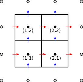
We remark that the box size $N$ (i.e., it contains $N^{D}$ cells) should typically be $8$ or higher, to reduce the overhead of storing neighbors, children, ghost cells and other information.

2.2 Defining the computational domain/coarse grid

After initializing the octree data structure, the user can specify a coarse grid consisting of one or more boxes together with their connectivity. To place two boxes next to each other, as in the example of figure 1, one could place the first one at index $(1,1)$ and the second one at $(2,1)$. If the neighbors of these two boxes are set to the special value af_no_box, their connectivity is automatically resolved. A periodic boundary in the $x$-direction can be imposed by specifying that the left neighbor of the first box is box two, and that the right neighbor of the second box is box one. External boundaries can be indicated by negative values. Besides rectangular grids, it is also possible to generate e.g., L-shaped meshes or O-shaped meshes containing a hole.

2.3 Mesh refinement

To adapt the mesh, the user has to specify a refinement routine. Given a box, this routine should specify a refinement flag for each cell: refine, derefine or keep refinement. Each mesh adaptation changes the mesh by at most one level at a given location. Boxes are either fully refined (with $2^{D}$ children) or not refined, but never partially refined. A number of rules is used to convert the cell-flags to refinement flags for the boxes:

• If any cell in a box is flagged for refinement, the box is refined. If neighbors of the box are at a lower refinement level, they are also refined to ensure 2:1 balance.

• Neighboring boxes within a distance of $N_{\mathrm{buf}}$ (default: two) cells of a cell flagged for refinement will also be refined. This also applies to diagonal neighbors.

• If all the cells in a box are marked for derefinement, then the box is marked for removal, but whether this happens depends on the points below:

  • If all the $2^{D}$ children of a box are flagged for removal, and the box itself not for refinement, then the children are removed.

  • Only leaves can be removed (because the grid changes by at most one level at a time).

  • Boxes cannot be removed if that would violate 2:1 balance.

When boxes are added or removed in the refinement procedure, the mesh connectivity is automatically updated, and the array containing all the boxes is automatically resized when necessary. The removal of boxes can create holes in this array, which are automatically filled when their number exceeds a threshold. The boxes are then also sorted (per level) according to their Morton index [21].

If a user has specified routines for prolongation (interpolation) and restriction of a cell-centered variable, then these operations are automatically performed when changing the mesh. The built-in prolongation and restriction routines are described in section 2.5. After updating the refinement, information on the added and removed boxes per level is returned, so a user can also manually set values on new boxes.

2.4 Ghost cells

The usage of ghost cells has two main advantages: algorithms can operate without special care for the boundaries, and they can do so in parallel. In Afivo each box always has one layer of ghost cells around its cell-centered variables. For numerical operations that depend on the nearest neighbors, such as computing a second order Laplacian or centered differences, one ghost cell is enough. When additional ghost values are required, these can directly be accessed due to the shared-memory parallelism.

Afivo supports a single layer of ghost cells around boxes, including corners (and edges in 3D). A user has to provide two routines for filling ghost cells on the sides of boxes, one for physical boundaries and one for refinement boundaries. A couple of such routines are also included with the framework. For each box, ghost cells are first filled on the sides, then on the edges (only present in 3D) and finally on the corners. For each side of a box, there are three options:

• If there is a neighbor at the same refinement level, copy from it.

• If there is a physical boundary, call the user’s routine for boundary conditions.

• If there is a refinement boundary, call the user’s routine for refinement boundaries.

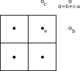
For the edge and corner ghost cells values are copied if a neighbor at the same refinement level is present. If there is no such neighbor, for example due to a physical or refinement boundary, these ghost cells are filled using linear extrapolation. The extrapolation procedure is illustrated in figure 3, for a corner ghost cell in 2D. A convenient property of this approach is that if one later uses bilinear interpolation using the points $(a,b,c,d)$ the result is equivalent to a linear interpolation based on points $(a,b,c)$. Furthermore, edge and corner ghost cells can be filled one box at a time, since they do not depend on ghost cells on neighboring boxes.

Figure 3: Illustration of the linear extrapolation procedure for corner ghost cells in 2D that is used when the diagonal neighbor is missing. The corner ghost cell gets a value $b+c-a$.

Afivo includes procedures to fill ghost cells near refinement boundaries using linear interpolation. Our approach allows users to construct custom schemes, which is important because there is no universal ‘correct’ way to do this: one has to balance higher order (to compensate for the increased discretization error near the refinement boundary) with conservation principles.

When a second layer of ghost cells is required, we temporarily copy a box to an enlarged version with two layers of ghost cells, as is also possible in Paramesh [16]. In principle, such an enlarged box could also be used for the first layer of ghost cells, so that no ghost cells need to be permanently stored. However, then one has to take care not to unnecessarily recompute ghost values, and extra storage is required to parallelize algorithms. Our approach of always storing a single layer of ghost cells therefore strikes a balance between memory usage, simplicity and performance.

2.5 Prolongation and restriction

In an AMR context, the interpolation of coarse grid values to obtain fine grid values is often called prolongation. The inverse procedure, namely the averaging of fine grid values to obtain coarse grid values, is called restriction.

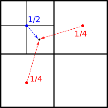
For prolongation, the standard bilinear and trilinear interpolation schemes are included. Furthermore, schemes with weights $(\tfrac{1}{2},\tfrac{1}{4},\tfrac{1}{4})$ (2D) and $(\tfrac{1}{4},\tfrac{1}{4},\tfrac{1}{4},\tfrac{1}{4})$ (3D) are included, as also implemented in e.g., Boxlib [22]. These linear schemes use information from the closest and second-closest coarse grid values, thereby avoiding the use of corner or edge ghost cell values. The 2D case is illustrated in figure 4. Zeroth-order interpolation, in which the coarse values are simply copied, is also implemented. The inclusion of higher order and conservative prolongation methods is left for future work.

As a restriction method Afivo includes averaging, in which the parent gets the average value of its children. A user can also implement custom interpolation and restriction methods.

Figure 4: Schematic drawing of $2-1-1$ interpolation. The three nearest coarse grid values are used to interpolate to the center of a fine grid cell. Note that the same interpolation scheme can be used for all fine grid cells, because of the symmetry in a cell-centered discretization.

2.6 OpenMP parallelism

Two conventional methods for parallel computing are OpenMP (shared memory) and MPI (communicating tasks). Afivo was designed for small scale parallelism, for example using 16 cores, and therefore only supports OpenMP. Compared to an MPI implementation, the use of OpenMP has several advantages: data can always be accessed, sequential (user) code can easily be included, and there is no need for load balancing or communication between processes. Furthermore, current systems often have 8 or more CPU cores and tens of gigabytes of RAM, which is sufficient for many scientific simulations. We remark that for problems requiring large scale parallelism, there are already a number of MPI-based frameworks available, see table 1.

Most operations in Afivo loop over a number of boxes, for example over the leaves at a certain refinement level. All such loops have been parallelized with OpenMP. In general, the parallel speedup depends on the cost of the algorithm that one is using. Because the communication cost (e.g., updating ghost cells) is always about the same, an expensive algorithm will show a better speedup. On shared memory systems, it is not unlikely for an algorithm to be memory-bound instead of CPU-bound.

2.7 Writing output

Afivo supports two output formats: VTK unstructured files and Silo files. The VTK unstructured format can handle much more general grids than quadtree and octree meshes. This format is therefore computationally more costly to visualize. Although there is some experimental support for octrees in VTK [23], this support does not yet seem to extend to data visualization programs such as Paraview [24] and Visit [25].

Afivo also supports writing Silo files, which include ghost cell information to prevent gaps in contour or surface plots. These files contain a number of Cartesian blocks (‘quadmeshes’ in Silo’s terminology). Because writing and reading a large number of separate blocks is quite costly, we use a simple algorithm to collect the leaf-boxes (those without children) at a refinement level into rectangular regions. The algorithm starts with a region $R$ that consists of a single box. If all the neighbors to the left of $R$ exist, have no children, and are not yet included in the output, then these neighbors are added to $R$; otherwise none of them is included. The procedure is repeated in all directions, until $R$ can no longer grow. Then $R$ is added to the output, and the procedure starts again until there are no leaf-boxes left.

3 Multigrid

Elliptic partial differential equations, such as Poisson’s equation, have to be solved in many applications. Multigrid methods [26, 27, 28, 29] can be used to solve such equations with great efficiency. The error in the solution is iteratively damped on a hierarchy of grids, with the coarse grids reducing the low frequency (i.e., long wavelength) error components, and the fine grids the high frequency components. When using adaptive mesh refinement on octree grids, geometric multigrid methods have several advantages:

• They can run in linear time, i.e., $O(N)$, where $N$ is the number of unknowns.

• Memory requirements are also linear in the number of unknowns.

• The octree already contains the hierarchy of grids required by the multigrid method.

• Geometric multigrid is matrix-free, so that changes in the mesh do not incur extra costs (direct methods would have to update their factorization).

For these reasons, we have implemented a geometric multigrid solver in Afivo, which can be used to solve problems of the form

$$A_{h}(u_{h})=\rho_{h},$$ (1)

where $A_{h}$ is a discretized elliptic operator, $\rho_{h}$ the source term, $u_{h}$ the solution to be computed and $h$ the mesh spacing. Boundary conditions can be of Dirichlet, Neumann or periodic type (or a mix of them). A drawback of geometric multigrid is that the operator $A_{h}$ also has to be well-defined on coarse grid levels. This complicates the implementation of e.g., irregular boundary conditions that do not align with the mesh.

On an octree mesh, the fine grid generally does not cover the whole domain. Therefore we use Full Approximation Scheme (FAS) version of multigrid, in which the solution is specified on all levels. The basic multigrid procedures are summarized below, with a focus on conservative discretization near refinement boundaries. A general introduction to multigrid methods can be found in e.g. [26, 27, 28].

3.1 Gauss-Seidel red-black smoother

A smoother, which locally smooths out the error in the solution, is a key component of a multigrid method. Afivo’s multigrid module comes with a collection of so-called Gauss-Seidel red-black smoothers, for Poisson’s equation in 2D, 3D and cylindrical coordinates. These methods operate on one box at a time, and can do so at any refinement level. How they work is explained below.

Consider an elliptic equation like (1) in 2D, using a 5-point numerical stencil. Such an equation relates a value $u_{h}^{(i,j)}$ at $(i,j$) to the source term $\rho^{(i,j)}$ and to neighboring values $u_{h}^{(i\pm 1,j)}$ and $u_{h}^{(i,j\pm 1)}$. If the values of the neighbors are kept fixed, the value $u_{h}^{(i,j)}$ that locally solves the equation can be determined. With Gauss-Seidel red-black, such a procedure is applied on a checkerboard pattern. In two dimensions, points $(i,j)$ can be labeled red when $i+j$ is even and black when $i+j$ is odd; the procedure is analogous for $(i,j,k)$ in 3D. The equation is then first solved for all the red points while keeping the old black values, and then for the black points.

For example, for Laplace’s equation with a standard second order discretization, a Gauss-Seidel red-black smoother replaces all red points by the average of their black neighbors, and then vice versa.

3.2 The V-cycle and FMG-cycle

There exist different multigrid cycles, which control in what order smoothers (of e.g. Gauss-Seidel red-black type) are used on different grid levels, and how information is communicated between these levels. The multigrid module of Afivo implement both the V-cycle and the FMG cycle; both can be called by users.

3.2.1 V-cycle

One of the most basic and standard ones is the V-cycle, which is included in Afivo. This cycle starts at the finest grid, descends to the coarsest grid, and then goes back up to the finest grid. Consider a grid with levels $l=1,2,\ldots,l_{\mathrm{max}}$. On each level $l$, $v_{h}$ denotes the current approximation to the solution on a grid spacing $h$, and $v_{H}$ refers to the (coarse) approximation on level $l-1$ with grid spacing $H=2h$. Furthermore, let $I_{H}^{h}$ be a prolongation operator to go from coarse to fine and $I_{h}^{H}$ a restriction operator to go from fine to coarse, as discussed in section 2.5. The FAS V-cycle can then be described as

1. For $l$ from $l_{\mathrm{max}}$ down to $2$, perform $N_{\mathrm{down}}$ (default: two) smoothing steps on level $l$, then compute the residual

   $$r_{h}=\rho_{h}-A_{h}(v_{h}).$$ (2)

   Afterwards update the level $l-1$ coarse grid:

   1. Set $v_{H}\leftarrow I_{h}^{H}v_{h}$, then store a copy $v^{\prime}_{H}$ of $v_{H}$.

   2. Update the coarse grid source term

      $$\rho_{H}\leftarrow I_{h}^{H}r_{h}+A_{H}(v_{H}).$$ (3)

2. Perform $N_{\mathrm{base}}$ (default: four) relaxation steps on level $1$, or apply a direct solver.

3. For $l$ from $2$ to $l_{\mathrm{max}}$, perform a correction using the data from level $l-1$

   $$u_{h}\leftarrow u_{h}+I_{H}^{h}(v_{H}-v^{\prime}_{H}),$$ (4)

   then perform $N_{\mathrm{up}}$ (default: two) relaxation steps on level $l$.

In step 2, relaxation takes place on the coarsest grid. In order to quickly converge to the solution with a relaxation method, this grid should contain very few points (e.g., $2\times 2$ or $4\times 4$ in 2D). Alternatively, a direct solver can be used on the coarsest grid, but such a solver is not yet included in Afivo. Currently, additional coarse grids are constructed below the coarsest quadtree/octree level. For example, if a quadtree has boxes of $16\times 16$ cells, then three coarser levels are added with boxes of $8\times 8$, $4\times 4$ and $2\times 2$ cells to speed up the multigrid convergence. Note that a non-square domain will contain more than one $2\times 2$ box on the coarse grid, and therefore require more coarse grid relaxation steps.

Successive V-cycles will reduce the residual $r_{h}$ on the different grid levels, see the example in section 4.1. No automatic error control has been implemented, so it is up to the user to decide when the residual is sufficiently small. The residual does typically not need to be reduced to zero, because the discretization error (due to the e.g. second order discretization) dominates when the residual is small enough. The number of V-cycles required to reach the discretization error is typically problem(-size) dependent.

3.2.2 FMG cycle

Besides the V-cycle, the full multigrid (FMG) cycle is also implemented in Afivo. An advantage of the FMG-cycle is that it typically gives convergence up to the discretization error in one or two iterations. The FMG-cycle operates as follows:

1. If there is no approximate solution yet, set the initial guess to zero on all levels, and restrict $\rho$ down to the coarsest grid using $I_{h}^{H}$. If there is an approximate solution $v$, restrict $v$ down to the coarsest level. Use equation (3) to set $\rho$ on coarse grids.

2. For $l=1,2,\ldots,l_{\mathrm{max}}$

   • Store the current approximation $v_{h}$ as $v^{\prime}_{h}$.

   • If $l>1$, perform a coarse grid correction using equation (4).

   • Perform a V-cycle starting at level $l$.

3.3 Conservative filling of ghost cells

As discussed in section 2.4, ghost cells are used to facilitate computations near refinement boundaries. How these ghost cells are filled affects the multigrid solution and convergence behavior. In Afivo, we have implemented conservative schemes for filling ghost cells [30, 27]. A conservative scheme ensures that the coarse flux across a refinement boundary equals the average of the fine fluxes, see figure 5. To illustrate why a conservative discretization is important, consider an equation of the form $\nabla\cdot\vec{F}=\rho$. The divergence theorem gives

$$\int_{V}\rho\,dV=\int_{V}\nabla\cdot\vec{F}\,dV=\int\vec{F}\cdot\vec{n}\,dS,$$ (5)

where the last integral runs over the surface of the volume $V$, and $\vec{n}$ is the normal vector to this surface. When the fine and coarse fluxes are consistent, the integral over $\rho$ will be same on the fine and the coarse grid.

Figure 5: Illustration of a refinement boundary. The cell centers are indicated by dots. There are two ghost values (gray dots) on the left of the refinement boundary. Fluxes across the refinement boundary are indicated by arrows.

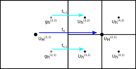
The construction of a conservative scheme for filling ghost cells is perhaps best explained with an example. Consider a 2D Poisson problem

$$\nabla^{2}u=\nabla\cdot(\nabla u)=\rho.$$

With a standard 5-point stencil for the Laplace operator the coarse flux $f_{H}$ across the refinement boundary in figure 5 is given by

$$f_{H}=[u_{H}^{(2,1)}-u_{H}^{(1,1)}]/H,$$

and on the fine grid, the two fluxes are given by

$$f_{h,1} =[u_{h}^{(3,1)}-g_{h}^{(2,1)}]/h,$$

$$f_{h,2} =[u_{h}^{(3,2)}-g_{h}^{(2,2)}]/h.$$

The task is now to fill the ghost cells $g_{h}^{(2,1)}$ and $g_{h}^{(2,2)}$ in such a way that the coarse flux equals the average of the fine fluxes:

$$f_{H}=(f_{h,1}+f_{h,2})/2.$$ (6)

To relate $u_{H}^{(2,1)}$ to the fine-grid values $u_{h}$, the restriction operator $I_{h}^{H}$ needs to be specified. In our implementation, this operator does averaging over the children. The constraint from equation (6) can then be written as

$$g_{h}^{(2,1)}+g_{h}^{(2,2)}=u_{H}^{(1,1)}+\frac{3}{4}\left(u_{h}^{(3,1)}+u_{h}^{(3,2)}\right)-\frac{1}{4}\left(u_{h}^{(4,1)}+u_{h}^{(4,2)}\right).$$ (7)

Any scheme for the ghost cells that satisfies this constraint leads to a conservative discretization.

Bilinear extrapolation (similar to standard bilinear interpolation) satisfies equation (7) and gives the following scheme for $g_{h}^{(2,1)}$

$$g_{h}^{(2,1)}=\frac{1}{2}u_{H}^{(1,1)}+\frac{9}{8}u_{h}^{(3,1)}-\frac{3}{8}\left(u_{h}^{(3,2)}+u_{h}^{(4,1)}\right)+\frac{1}{8}u_{h}^{(4,2)}.$$

(The scheme for $g_{h}^{(2,2)}$ follows from symmetry.) Another option is to use only the closest two neighbors for the extrapolation, which gives the following expression for $g_{h}^{(2,1)}$

$$g_{h}^{(2,1)}=\frac{1}{2}u_{H}^{(1,1)}+u_{h}^{(3,1)}-\frac{1}{4}\left(u_{h}^{(3,2)}+u_{h}^{(4,1)}\right).$$

This last scheme is how ghost cells at refinement boundaries are filled by default in Afivo. In three dimensions, the scheme becomes

$$g_{h}^{(2,1,1)}=\frac{1}{2}u_{H}^{(1,1,1)}+\frac{5}{4}u_{h}^{(3,1,1)}-\frac{1}{4}\left(u_{h}^{(4,1,1)}+u_{h}^{(3,2,1)}+u_{h}^{(3,1,2)}\right).$$

We have observed that filling ghost cells as described above can reduce the multigrid convergence rate, in particular in 3D. There are two reasons: first, a type of local extrapolation is performed, and the larger the coefficients in this extrapolation are, the more smoothing is required to reduce errors. Second, cells near a refinement boundary do not locally solve the linear equation after an Gauss-Seidel red-black update, if one takes into account that the ghost cells also have to be updated. It is possible to fix this, in a similar way as one can change the stencil near physical boundaries instead of using ghost cells, but near a ‘refinement corner’ the situation is more complicated.

3.4 Including discontinuities in $\varepsilon$

For the more general equation $\nabla\cdot(\varepsilon\nabla\phi)=\rho$ we have implemented a special case: $\varepsilon$ jumps from $\varepsilon_{1}$ to $\varepsilon_{2}$ at a cell face. Local reconstruction of the solution shows that the flux through the cell face is then given by

$$\frac{2\,\varepsilon_{1}\varepsilon_{2}}{\varepsilon_{1}+\varepsilon_{2}}\,\frac{\phi_{i+1}-\phi_{i}}{h}.$$ (8)

In other words, the flux is multiplied by the harmonic mean of the $\varepsilon$’s (see e.g., chapter 7.7 of [27]). The ghost cell schemes described above for constant $\varepsilon$ still ensure flux conservation, because the coarse and fine flux are multiplied by the same factor. The jump should occur at a cell face at all refinement levels, which is equivalent to requiring that it occurs at a coarse grid cell face.

3.5 Supported operators

The following elliptic operators have been implemented in Afivo:

• 2D/3D Laplacian in Cartesian coordinates, using a 5 and 7-point stencil respectively.

• 2D/3D Laplacian with a jump in coefficient on a cell face, as discussed in the previous section. A custom prolongation (interpolation) method that uses the locally reconstructed solution is also included.

• Cylindrical Laplacian in $(r,z)$-coordinates, also supporting a jump in coefficient on a cell face.

Furthermore, a Laplacian with support for internal boundaries has been implemented, which makes use of a level set function to determine the location of the boundaries. At the moment, this only works if the boundary can also be resolved on the coarse grid. The future implementation of a direct sparse method for the coarse grid equations will enable this functionality more generally, because the coarse grid can then have a higher resolution.

Users can also define custom elliptic operators, as well as custom smoothers and prolongation and restriction routines. One of the examples included with Afivo shows how the diffusion equation $\partial_{t}n=D\nabla^{2}n$ can be solved with a backward Euler scheme by defining such a custom operator.

4 Examples

Several examples that demonstrate how to use Afivo are included in the examples folder of Afivo’s source code, see section 1.1. Here we discuss a few of the examples in detail.

4.1 Multigrid convergence

Figure 6: Left: mesh spacing used for the multigrid examples, in a $[0,1]\times[0,1]$ domain. Black indicates $\Delta x=2^{-11}$ and white $\Delta x=2^{-5}$. Right: the maximum residual and maximum error versus FMG iteration. Case 1 corresponds to a standard Laplacian (equation (9)) and case 2 to the cylindrical case with a jump in $\varepsilon$ (equation (10)).

In this section we present two test problems to demonstrate the multigrid behavior on a partially refined mesh. We use the method of manufactured solutions: from an analytic solution the source term and boundary conditions are computed. Two test problems are considered, a constant-coefficient Poisson equation in 2D

$$\nabla^{2}u=\nabla\cdot(\nabla u)=\rho$$ (9)

and a problem with cylindrical symmetry in $(r,z)$ coordinates

$$\frac{1}{r}\partial_{r}(r\varepsilon\partial_{r}u)+\partial_{z}(\varepsilon\partial_{z}u)=\rho,$$ (10)

both on a two-dimensional rectangular domain $[0,1]\times[0,1]$. For the second case, $\varepsilon$ has a value of $100$ in the lower left quadrant $[0,0.25]\times[0,0.25]$, and a value of $1$ in the rest of the domain. In both cases, we pick the following solution for $u$

$$u(r)=\exp(\left|\vec{r}-\vec{r}_{1}\right|/\sigma)+\exp(\left|\vec{r}-\vec{r}_{2}\right|/\sigma),$$ (11)

where $\vec{r_{1}}=(0.25,0.25)$, $\vec{r_{2}}=(0.75,0.75)$ and $\sigma=0.04$. An analytic expression for the source term $\rho$ is obtained by plugging the solution in equations (9) and (10) (note that jumps in $\varepsilon$ also contribute to the source term $\rho$). The solution is used to set Dirichlet boundary conditions. For these examples, we have used $N_{\mathrm{down}}=2$, $N_{\mathrm{up}}=2$ and $N_{\mathrm{base}}=4$ smoothing steps, and boxes with $8^{2}$ cells.

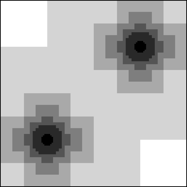
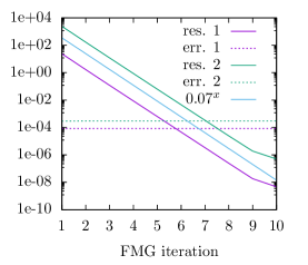
The refinement criterion is based on the source term $\rho$: refine if $\Delta x^{2}|\rho|/\varepsilon>10^{-3}$, where $\varepsilon$ is one for the first problem. The resulting mesh spacing, which is the same for both problems, is shown in figure 6a. Figure 6b shows that in both cases, one FMG (full multigrid) cycle is enough to achieve convergence up to the discretization error. Consecutive FMG cycles further reduce the residual $r=\rho-\nabla^{2}u$. The convergence behavior is similar for both cases, with each iteration reducing the residual by a factor of about $0.07$. This factor decreases when more smoothing steps are taken and when a higher order prolongation or restriction method is used. For this example we have used first order prolongation and simple averaging for restriction, as discussed in section 2.5. The offset between the lines is caused by the $\varepsilon=100$ region, which locally amplifies the source term by a factor of 100.

4.2 Multigrid performance and scaling

Figure 7: Duration (left) and speedup (right) of a single FMG cycle on a uniformly refined grid of $512^{3}\approx 134\times 10^{6}$ cells versus the number of OpenMP threads. Results are shown for octrees with boxes of $8^{3}$, $16^{3}$ and $32^{3}$ cells.

Here we briefly investigate the performance and scaling of the multigrid routines. Although the numbers presented here depend on the particular system and compiler used, they can be used to estimate feasible problem sizes with Afivo. As a performance test we use a 3D Poisson problem

$$\nabla^{2}\phi=1,$$

on a domain $[0,1]^{3}$ with $\phi=0$ at the boundaries. For simplicity (and for comparison with other methods), the domain is uniformly refined up to a resolution of $512^{3}$ cells.

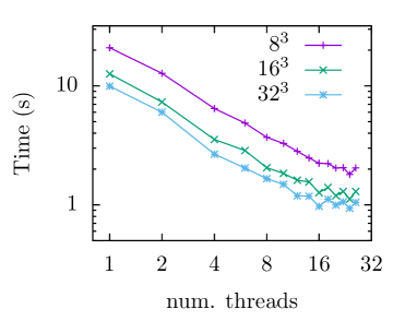
Figure 7 shows the duration of a single FMG cycle versus the number of processor cores used, again using $N_{\mathrm{down}}=2$, $N_{\mathrm{up}}=2$ and $N_{\mathrm{base}}=4$ smoothing steps. Curves are shown for box sizes of $8^{3}$, $16^{3}$ and $32^{3}$, which affect the overhead of the adaptive octree mesh. The runs were performed on a node with Xeon E5-2680 processors ($2.8\,\textrm{GHz}$, 20 cores per node).

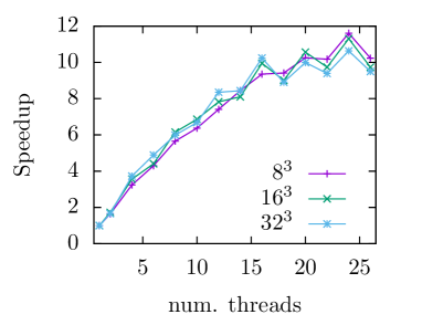
The maximal speedups are about $4.9$ ($8^{3}$ case), $5.4$ ($16^{3}$ case) and $5.7$ ($32^{3}$ case). The performance of the geometric multigrid algorithm, which performs only a few additions and multiplications per cell during each smoothing step, is probably bound by the memory bandwidth of the system. We also see that performance is increased when using larger boxes, because this reduces the overhead due to the filling of ghost cells. For the $32^{3}$ case with 16 cores, the time spent per unknown is about $10\,\textrm{ns}$, whereas it is about $22\,\textrm{ns}$ for the $8^{3}$ case with 16 cores.

4.3 Discharge model

In previous studies [11, 12], Afivo has already been used to study the guiding of so-called streamer discharges in 3D. For simplicity, we here consider a simpler 2D plasma fluid model for electric gas discharges [8]. This model is used to simulate the destabilization of a planar ionization wave in pure nitrogen, in a background field above the breakdown threshold. The destabilization of such planar ionization waves has been investigated mainly analytically in the past [31, 32, 33].

The model is kept as simple as possible: it contains only electrons and positive ions, no photo-ionization and no plasma chemistry. The evolution of the electron and ion density ($n_{e}$ and $n_{i}$) is then described by the following equations:

$$\partial_{t}n_{e} =\nabla\cdot(\mu_{e}\vec{E}n_{e}+D_{e}\nabla n_{e})+\alpha(E)\mu_{e}En_{e},$$ (12)

$$\partial_{t}n_{i} =\alpha(E)\mu_{e}En_{e},$$ (13)

$$\nabla^{2}\phi =-e(n_{i}-n_{e})/\varepsilon_{0},\qquad\vec{E}=-\nabla\phi,$$ (14)

where $\mu_{e}$ is the electron mobility, $D_{e}$ the electron diffusion coefficient, $\alpha(E)$ the ionization coefficient, $\vec{E}$ the electric field, $\phi$ the electrostatic potential, $\varepsilon_{0}$ the permittivity of vacuum and $e$ the elementary charge. The motion of ions is not taken into account here. The electrostatic potential is computed with the FMG multigrid routine described in section 3.2. The electric field at cell faces is then calculated by taking central differences.

For simplicity, we use a constant mobility $\mu_{e}=0.03\,\textrm{m}^{2}/(\mathrm{Vs})$, a constant diffusion coefficient $D_{e}=0.2\,\textrm{m}^{2}/\mathrm{s}$ and we take an analytic expression for the ionization coefficient $\alpha(E)=\exp\left[10.4+0.601\log(E/E^{*})-186(E^{*}/E)\right]$, with $E^{*}=1\,\textrm{kV/cm}$ [7]. These coefficients roughly correspond to nitrogen at room temperature and normal pressure. In a more realistic model, one would typically include tabulated transport coefficients to make the results more realistic. Such coefficients can be computed with a Boltzmann solver (e.g., [34, 35]) or particle swarms (e.g., [36, 37]).

The electron flux is computed as in [6]. The diffusive part is computed using central differences and the drift part is computed using the Koren limiter [1]. The Koren limiter was not designed to include refinement boundaries, and we use linear interpolation to obtain fine-grid ghost values. These ghost cells lie inside a coarse-grid neighbor cell, and we limit them to twice the coarse values to preserve positivity.

Time stepping is also performed as in [6], using the explicit trapezoidal rule. The global time step is taken as the minimum over the cells of

• CFL condition: $\frac{1}{2}/\left(|v_{x}|/\Delta x+|v_{y}|/\Delta x\right)$, where $v_{x}$ and $v_{y}$ are the $x$ and $y$-component of the electron drift

• Explicit diffusion limit: $\Delta x^{2}/(4D_{e})$

• Dielectric relaxation time: $\varepsilon_{0}/(e\mu_{e}n_{e})$

The refinement criterion is based on the ionization coefficient $\alpha$, which depends on the local electric field. The reasoning behind this is that $1/\alpha$ is a typical length scale for the electron and ion density gradients and the width of space charge layers [33]. Where $n_{e}>1\,\textrm{m}^{-3}$ (an arbitrary small value) and $\alpha\Delta x>0.8$, the mesh is marked for refinement. Elsewhere the mesh is marked for derefinement when $\Delta x<25\,\mu\textrm{m}$ and $\alpha\Delta x<0.1$. The quadtree mesh for this example was constructed from boxes containing $8^{2}$ cells.

Figure 8: The evolution of the electron density (top) and electric field (bottom) in a 2D electric discharge simulation in nitrogen at standard temperature and pressure. The discharge started from a pre-ionized layer, which destabilizes into streamer channels. A zoom-in of the mesh around a streamer head at $t=8\,\textrm{ns}$ is shown in figure 9.

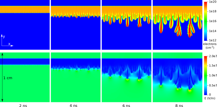
The model described above is used to simulate discharges in a domain of $(1\,\textrm{cm})^{2}$, see figure 8. Initially, a density $n_{0}$ of approximately $10^{15}\,\textrm{cm}^{-3}$ electrons and ions is present between $y=9\,\textrm{mm}$ and $y=9.5\,\textrm{mm}$, elsewhere the density is zero. The precise density in each cell is drawn using random numbers, by taking samples from a normal distribution with mean and variance $n_{0}\Delta x^{3}$, with $\Delta x\approx 9.8\mu\mathrm{m}$ in the region of the initial condition. For $n_{0}\Delta x^{3}\gg 1$, as we have here, this approximates the Poisson distribution of physical particle noise (when the simulation would be truly 3D). At $y=1\,\textrm{cm}$ the domain is grounded, and at $y=0$ a background field of $8\,\textrm{MV/m}$ is applied through a Neumann condition for the electric potential; therefore the electrons drift downward in the field. The electron and ion density at the $y$-boundaries are set to zero, and the domain has periodic boundary conditions in the $x$-direction.

Figure 8 shows how the electron density and the electric field evolve in time. At first, the pre-ionized layer grows rather homogeneously downwards due to electron drift and creation of more charges through impact ionization, but because small inhomogeneities locally enhance the electric field [33], the layer quickly destabilizes into streamer channels. The faster channels electrically screen the slower ones, reducing the number of active channels over time. Figure 9 shows a zoom of the adaptively refined mesh at $t=8\,\textrm{ns}$.

Figure 9: The full domain and a 50 times zoom, which shows the electric field and the mesh around a streamer head at $t=8\,\textrm{ns}$. The finest grid spacing is $\Delta x\approx 1.22\,\mu\textrm{m}$.

4.4 Toy model of particles interacting through gravity

Afivo includes basic functionality for particle simulations. A bi/tri-linear interpolation procedure is provided to interpolate fields at particle positions. There is also a routine for mapping a list of particle coordinates and corresponding weights to densities on a grid. Particles can be assigned to the nearest cell center, or a cloud-in-cell shape function [38] can be used.

To demonstrate the particle coupling, we present results of a simple toy model for self-gravitating particles in a fully periodic domain. The model is inspired by N-body codes for gravitating systems [39]. Here we do not take the short-range interaction between particles into account, and the model does not strictly conserve energy. For simplicity, we omit all units in the model’s description below and we set $4\pi G=1$, where $G$ is the gravitational constant.

Figure 10: Evolution of the mass density in a 3D periodic system with $10^{8}$ particles interacting through gravity. Initially, the particles were uniformly distributed. The visualization was made with Visit [25], using volume rendering.

Initially, $10^{8}$ particles are uniformly distributed over a unit cube, using pseudorandom numbers. The initial velocities are set to zero. Each particle has a mass of $10^{-8}$, so that the mean mass density is one. At each time step, particle positions and velocities are updated using a synchronized leapfrog scheme:

$$\mathbf{x}_{t+1/2} =\mathbf{x}_{t}+\tfrac{1}{2}\Delta t\,\mathbf{v}_{t},$$

$$\mathbf{v}_{t+1} =\mathbf{v}_{t}+\tfrac{1}{2}\Delta t\,\mathbf{g}_{t+1/2},$$

$$\mathbf{x}_{t+1} =\mathbf{x}_{t+1/2}+\tfrac{1}{2}\Delta t\,\mathbf{v}_{t+1}.$$

The gravitational acceleration $\mathbf{g}_{t+1/2}$ is computed by central differencing of the gravitational potential $\mathbf{g}_{t+1/2}=-\nabla\phi_{t+1/2}$, and $\phi$ is obtained by solving Poisson’s equation

$$\nabla^{2}\phi_{t+1/2}=\rho_{t+1/2}-\bar{\rho},\\$$

where $\rho_{t+1/2}$ is the mass density at $t+1/2$. The mean mass density $\bar{\rho}$ is subtracted to ensure a fully periodic solution exists, as it follows from the divergence theorem that the integrated source term has to be zero.

During the simulation, the mesh is refined where cells contain more than 100 simulation particles, and refinement is removed when boxes contain less than 4 particles. At most seven refinement levels are used, so that the finest grid has a spacing of about $2\cdot 10^{-3}$. A constant time step $\Delta t=10^{-2}$ is used. Figure 10 shows the evolution of the mass density up to $t=5$. Small fluctuations in the initial particle density grow over time, and eventually dense and dilute regions form a complex structure. Up to $t=3$, the domain contains about $2$ million cells, but as more and more fine-scale structure forms, about $10^{8}$ cells are used at $t=5$.

5 Conclusion & outlook

This paper describes Afivo, a framework for parallel simulations on adaptively refined quadtree/octree grids with a geometric multigrid solver. We have tried to keep the framework simple to facilitate modification, so it can be used to experiment with AMR algorithms and methods. An overview of Afivo’s main data structures and procedures was given, and the included geometric multigrid solvers have been described. We have presented examples of the multigrid convergence and scaling, of a simplified discharge model in 2D, and of a toy model for gravitationally interacting particles in 3D.

Future developments will focus on the inclusion of a sparse direct solver that can handle the coarse grid of the multigrid procedure. This will make it easier to include irregular boundary conditions in the multigrid solver, to enable for example the inclusion of curved electrodes in electrostatic calculations.

Acknowledgments We thank Margreet Nool for her help with the documentation and the examples. While developing Afivo, JT was supported by project 10755 of the Dutch Technology Foundation STW, which is part of the Netherlands Organisation for Scientific Research (NWO), and which is partly funded by the Ministry of Economic Affairs. JT is now supported by postdoctoral fellowship 12Q6117N from Research Foundation – Flanders (FWO).

References

- Koren [1993] B. Koren, in: C. Vreugdenhil, B. Koren (Eds.), Numerical Methods for Advection-Diffusion Problems, Braunschweig/Wiesbaden: Vieweg, 1993, pp. 117–138.
- Vitello et al. [1994] P. A. Vitello, B. M. Penetrante, J. N. Bardsley, Physical Review E 49 (1994) 5574–5598. URL: http://dx.doi.org/10.1103/PhysRevE.49.5574. doi:10.1103/physreve.49.5574.
- Yi and Williams [2002] W. J. Yi, P. F. Williams, J. Phys. D: Appl. Phys. 35 (2002) 205–218. URL: http://dx.doi.org/10.1088/0022-3727/35/3/308. doi:10.1088/0022-3727/35/3/308.
- Ebert et al. [2010] U. Ebert, S. Nijdam, C. Li, A. Luque, T. Briels, E. van Veldhuizen, Journal of Geophysical Research 115 (2010). URL: http://dx.doi.org/10.1029/2009JA014867. doi:10.1029/2009ja014867, a00E43.
- Pancheshnyi et al. [2008] S. Pancheshnyi, P. Ségur, J. Capeillère, A. Bourdon, Journal of Computational Physics 227 (2008) 6574–6590. URL: http://dx.doi.org/10.1016/j.jcp.2008.03.020. doi:10.1016/j.jcp.2008.03.020.
- Montijn et al. [2006] C. Montijn, W. Hundsdorfer, U. Ebert, Journal of Computational Physics 219 (2006) 801–835. URL: http://dx.doi.org/10.1016/j.jcp.2006.04.017. doi:10.1016/j.jcp.2006.04.017.
- Li et al. [2012] C. Li, U. Ebert, W. Hundsdorfer, Journal of Computational Physics 231 (2012) 1020–1050. URL: http://dx.doi.org/10.1016/j.jcp.2011.07.023. doi:10.1016/j.jcp.2011.07.023.
- Luque and Ebert [2012] A. Luque, U. Ebert, Journal of Computational Physics 231 (2012) 904–918. URL: http://dx.doi.org/10.1016/j.jcp.2011.04.019. doi:10.1016/j.jcp.2011.04.019.
- Kolobov and Arslanbekov [2012] V. Kolobov, R. Arslanbekov, Journal of Computational Physics 231 (2012) 839–869. URL: http://dx.doi.org/10.1016/j.jcp.2011.05.036. doi:10.1016/j.jcp.2011.05.036.
- Popinet [2003] S. Popinet, Journal of Computational Physics 190 (2003) 572–600. URL: http://dx.doi.org/10.1016/S0021-9991(03)00298-5. doi:10.1016/s0021-9991(03)00298-5.
- Nijdam et al. [2016] S. Nijdam, J. Teunissen, E. Takahashi, U. Ebert, Plasma Sources Science and Technology 25 (2016) 044001. URL: http://dx.doi.org/10.1088/0963-0252/25/4/044001. doi:10.1088/0963-0252/25/4/044001.
- Teunissen and Ebert [2017] J. Teunissen, U. Ebert, Journal of Physics D: Applied Physics 50 (2017) 474001. URL: http://dx.doi.org/10.1088/1361-6463/aa8faf. doi:10.1088/1361-6463/aa8faf.
- Zhang et al. [2016] W. Zhang, A. Almgren, M. Day, T. Nguyen, J. Shalf, D. Unat, SIAM Journal on Scientific Computing 38 (2016) S156–S172. URL: http://dx.doi.org/10.1137/15M102616X. doi:10.1137/15m102616x.
- Colella et al. [2011] P. Colella, D. T. Graves, J. N. Johnson, N. D. Keen, T. J. Ligocki, D. F. Martin, P. W. McCorquodale, D. Modiano, P. O. Schwartz, T. D. Sternberg, B. V. Straalen, Chombo software package for AMR applications - design document, 2011. URL: https://apdec.org/designdocuments/ChomboDoc/ChomboDesign/chomboDesign.pdf.
- Hornung et al. [2006] R. D. Hornung, A. M. Wissink, S. R. Kohn, Engineering with Computers 22 (2006) 181–195. URL: http://dx.doi.org/10.1007/s00366-006-0038-6. doi:10.1007/s00366-006-0038-6.
- MacNeice et al. [2000] P. MacNeice, K. M. Olson, C. Mobarry, R. de Fainchtein, C. Packer, Computer Physics Communications 126 (2000) 330–354. URL: http://dx.doi.org/10.1016/S0010-4655(99)00501-9. doi:10.1016/s0010-4655(99)00501-9.
- Sampath et al. [2008] R. S. Sampath, S. S. Adavani, H. Sundar, I. Lashuk, G. Biros, 2008 SC - International Conference for High Performance Computing, Networking, Storage and Analysis (2008). URL: http://dx.doi.org/10.1109/SC.2008.5218558. doi:10.1109/sc.2008.5218558.
- Weinzierl [2009] T. Weinzierl, A Framework for Parallel PDE Solvers on Multiscale Adaptive Cartesian Grids, Technische Universität München, 2009.
- Teyssier [2002] R. Teyssier, A&A 385 (2002) 337–364. URL: http://dx.doi.org/10.1051/0004-6361:20011817. doi:10.1051/0004-6361:20011817.
- Calhoun [2015] D. Calhoun, Adaptive mesh refinement resources, 2015. URL: http://math.boisestate.edu/~calhoun/www_personal/research/amr_software/index.html, [Online; accessed 18-April-2018].
- Morton [1966] G. Morton, IBM Research Report (1966).
- et al. [2015] A. S. A. et al., Boxlib, 2015. URL: https://ccse.lbl.gov/BoxLib/index.html, [Online; accessed 22-July-2015].
- Carrard et al. [2012] T. Carrard, C. Law, P. Pébay, 21st International Meshing Roundtable (2012).
- Kitware [2015] Kitware, Paraview, 2015. URL: https://www.paraview.org/, [Online; accessed 20-April-2018].
- Childs et al. [2012] H. Childs, E. Brugger, B. Whitlock, J. Meredith, S. Ahern, D. Pugmire, K. Biagas, M. Miller, C. Harrison, G. H. Weber, H. Krishnan, T. Fogal, A. Sanderson, C. Garth, E. W. Bethel, D. Camp, O. Rübel, M. Durant, J. M. Favre, P. Navrátil, in: High Performance Visualization–Enabling Extreme-Scale Scientific Insight, Chapman and Hall/CRC, 2012, pp. 357–372.
- Brandt and Livne [2011] A. Brandt, O. E. Livne, Multigrid Techniques, Society for Industrial & Applied Mathematics (SIAM), 2011. URL: http://dx.doi.org/10.1137/1.9781611970753. doi:10.1137/1.9781611970753.
- Trottenberg et al. [2000] U. Trottenberg, C. Oosterlee, A. Schuller, Multigrid, Elsevier Science, 2000.
- Briggs et al. [2000] W. L. Briggs, V. E. Henson, S. F. McCormick, A Multigrid Tutorial (2nd Ed.), Society for Industrial & Applied Mathematics, Philadelphia, PA, USA, 2000.
- Hackbusch [1985] W. Hackbusch, Springer Series in Computational Mathematics (1985). URL: http://dx.doi.org/10.1007/978-3-662-02427-0. doi:10.1007/978-3-662-02427-0.
- Bai and Brandt [1987] D. Bai, A. Brandt, SIAM Journal on Scientific and Statistical Computing 8 (1987) 109–134. URL: http://dx.doi.org/10.1137/0908025. doi:10.1137/0908025.
- Arrayás and Ebert [2004] M. Arrayás, U. Ebert, Physical Review E 69 (2004). URL: http://dx.doi.org/10.1103/PhysRevE.69.036214. doi:10.1103/physreve.69.036214.
- Derks et al. [2008] G. Derks, U. Ebert, B. Meulenbroek, J Nonlinear Sci 18 (2008) 551–590. URL: http://dx.doi.org/10.1007/s00332-008-9023-0. doi:10.1007/s00332-008-9023-0.
- Ebert et al. [2010] U. Ebert, F. Brau, G. Derks, W. Hundsdorfer, C.-Y. Kao, C. Li, A. Luque, B. Meulenbroek, S. Nijdam, V. Ratushnaya, et al., Nonlinearity 24 (2010) C1–C26. URL: http://dx.doi.org/10.1088/0951-7715/24/1/C01. doi:10.1088/0951-7715/24/1/c01.
- Hagelaar and Pitchford [2005] G. J. M. Hagelaar, L. C. Pitchford, Plasma Sources Science and Technology 14 (2005) 722–733. URL: http://dx.doi.org/10.1088/0963-0252/14/4/011. doi:10.1088/0963-0252/14/4/011.
- Dujko et al. [2011] S. Dujko, U. Ebert, R. D. White, Z. L. Petrović, Japanese Journal of Applied Physics 50 (2011) 08JC01. URL: http://dx.doi.org/10.1143/JJAP.50.08JC01. doi:10.1143/jjap.50.08jc01.
- Li et al. [2010] C. Li, U. Ebert, W. Hundsdorfer, Journal of Computational Physics 229 (2010) 200–220. URL: http://dx.doi.org/10.1016/j.jcp.2009.09.027. doi:10.1016/j.jcp.2009.09.027.
- Rabie and Franck [2016] M. Rabie, C. Franck, Computer Physics Communications 203 (2016) 268–277. URL: http://dx.doi.org/10.1016/j.cpc.2016.02.022. doi:10.1016/j.cpc.2016.02.022.
- Hockney and Eastwood [1988] R. W. Hockney, J. W. Eastwood, Computer simulation using particles., IOP Publishing Ltd., Bristol, England, 1988.
- Dehnen and Read [2011] W. Dehnen, J. I. Read, The European Physical Journal Plus 126 (2011). URL: http://dx.doi.org/10.1140/epjp/i2011-11055-3. doi:10.1140/epjp/i2011-11055-3.
- Ripperda et al. [2018] B. Ripperda, F. Bacchini, J. Teunissen, C. Xia, O. Porth, L. Sironi, G. Lapenta, R. Keppens, The Astrophysical Journal Supplement Series 235 (2018) 21. URL: http://dx.doi.org/10.3847/1538-4365/aab114. doi:10.3847/1538-4365/aab114.