Light Source Estimation with Analytical Path-tracing

Abstract

We present a novel algorithm for light source estimation in scenes reconstructed with a RGB-D camera based on an analytically-derived formulation of path-tracing. Our algorithm traces the reconstructed scene with a custom path-tracer and computes the analytical derivatives of the light transport equation from principles in optics. These derivatives are then used to perform gradient descent, minimizing the photometric error between one or more captured reference images and renders of our current lighting estimation using an environment map parameterization for light sources. We show that our approach of modeling all light sources as points at infinity approximates lights located near the scene with surprising accuracy. Due to the analytical formulation of derivatives, optimization to the solution is considerably accelerated. We verify our algorithm using both real and synthetic data.

I Introduction

Computer vision is often referred to as the “inverse graphics” problem. This is because many of the equations and relations used in computer vision find their roots in the understanding of image formation and light interaction. However the complete process of image formation is mainly ignored in most applications of computer vision. In the case of localization and mapping, brightness constancy is assumed from multiple viewpoints and robust estimation is used to reduce or ignore the influence of any non-cooperative observations. While this approach works well for surfaces exhibiting Lambertian reflectivity, specular and transparent surfaces are often treated as outliers. This assumptions is also the cause of the complexity of localization from a completely dense 3D map. While brightness constancy may apply from small baselines, it generally does not in the case of widely varying baselines.

These approximations inhibit the estimation of many quantities of interest, such as light position, sensor response curves, and surface properties of in-scene objects. The light position estimation problem itself has garnered significant interest in the autonomous robotics community. Dynamic shadow effects for instance stymie feature- and deep learning-based algorithms for place and object recognition. [4] proposed a filter-based approach to this problem which removes shadows from images, but struggles with shadows containing reflected light and artificial light sources, such as lamps or headlights. The assumption of constant illumination is critical to tracking applications [22], which could be potentially improved through the consideration of irregular illumination imbued by individual light sources as well.

A number of previous works have handled in-scene light source position estimation. For instance, Elastic Fusion [22] introduces a method for this via ray casting and tessellating the space with potential light source voxels with a merging function. This method precludes the estimation of surface reflectancies however, as ray casting requires that they are provided at the outset. As an alternative to using potential light emitting voxels, an “environment map” may instead be employed to represent light sources. This approach imposes an encapsulating 2-manifold (typically a hemisphere) around the 3-dimensional region of interest and parametrizes a coordinate system on the manifold that act as inwardly-directed point light sources [9, 13].

A number of approaches have been taken on estimating the effect of in-scene lighting with considerable success. For instance, [14] addresses light source estimation by laying out a light-field which can then be used for casting shadows. The light sources in this case do not follow a physically derived model, but recreate in-scene lighting with impressive accuracy. A different approach is applied by [12], where a learned set of radiance transfer functions are applied for generating plausible lighting incident on a human face. Meanwhile, there has been steady development in approaches to estimating light effects for out-of-scene sources, e.g. [24, 21, 8, 2]. These approaches may be used to e.g. cast artificial shadows for the purposes of augmented reality, but do not admit the arbitrary estimation of in-scene parameters.

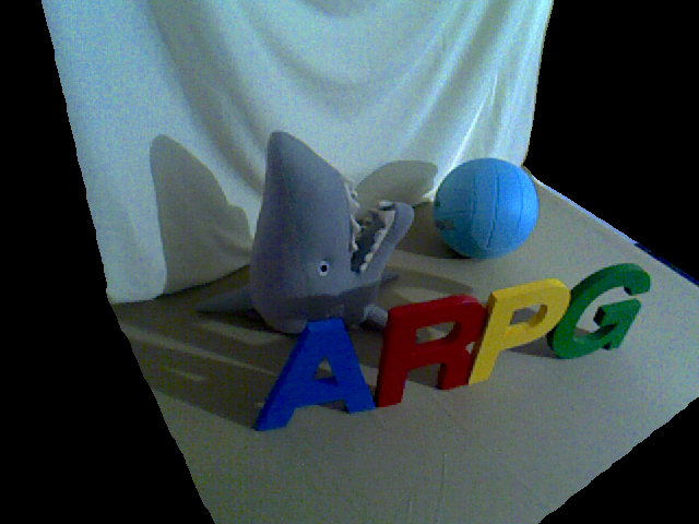
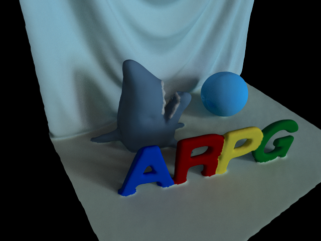
Figure 1: Left: captured reference image, Right: render of estimated lighting conditions found using our algorithm

To address these limitations, optical path tracing may be employed to both estimate scene parameters as well as for photorealistic rendering, including the effects of lens flares, specular highlights, shadows, and other visual phenomena. This approach applies a generative model for light interaction with a scene using methods from optics, and admits the selective approximation as need warrants. Path tracing however has proven to be a prohibitively computationally expensive solution, as path tracing is a nonlinear operation with a thousands of optimization parameters.

The method described in this paper eschews the use of finite differences in favor of analytical derivatives of the light transport equation. We use an environment map parametrization of light sources and employ robust nonlinear optimization in order to estimate the position of light sources in a scene. Our process is naturally extensible to the estimation of scene properties including surface reflectivity. We give a description of our method in Sections II-V. Our results are provided in Section VI and discussed in Section VII. We draw conclusions from our work in Section VIII.

II Overview

Physically-based rendering refers to the process of image formation that remains as faithful to real-world optics as possible. This is achieved through accurately modeling the interaction of light with the surfaces and volumes in our scene. Such rendering engines are often referred to as path-tracers, as they simulate the path an emitted ray of light takes as it traverses the scene before eventually being captured by our synthetic image sensor. As the vast majority of light in the scene will never actually reach the image sensor, this problem is typically inverted for the sake of computational simplicity. So we instead trace rays of light from the image sensor back to the light source. In order to synthesize high-fidelity images with little to no noise, hundreds or thousands of rays must be traced for every pixel. These general concepts are illustrated in Figure 2.

The most important concept to take away from all of this, in regards to the work presented in this paper, is that while this process requires tracing thousands of rays, intersecting them with the scene geometry at each bounce, computing the material properties and angles of incidence at each point of intersection, as the rays make their way towards a light source, all of the geometry, material properties, and math compute a single coefficient which denotes the amount of light from a given light source that is stored in a given pixel. This idea sits at the heart of our algorithm.

We leverage this fact in our formulation of the light estimation problem. A custom path-tracer generates these coefficients for each pixel-light pair. We use these values to compose a linear system of equations that can be solved using standard optimization techniques. The power of this approach is that not only can it be gracefully extended to handle any optical phenomema that could be present in our observed scene, it can also be rewritten to solve for different components of image formation.

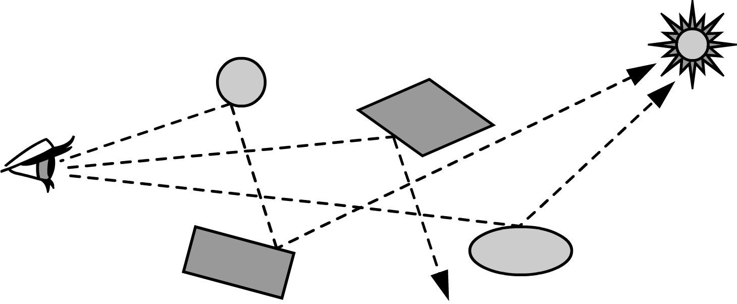
Figure 2: Path-tracing models how rays of light traverse a given scene. With each collision with the scene’s geometry, information about surface materials, angle of incidence, and location of the light source are used to compute the amount of light reaching the synthetic camera sensor.

III Scene Model

We now describe the input required by our algorithm for performing path-tracing and estimating the lighting conditions in the observed scene.

III-A 3D Geometry

In order to properly simulate how rays emitted from light sources bounce off surfaces before reaching our camera we first require a 3D geometric representation of the scene. Our implementation uses a triangle mesh with corresponding surface normals as seen in Figure 3(a). We capture such a mesh using a Asus Xtion Pro Live and the InfiniTam 3D reconstruction framework [10]. The more complete this reconstruction is the better we can recreate shadows and simulate how light bounces around the surfaces of the scene. However we have observed that even largely incomplete reconstructions still afford accurate light source estimation.

III-B Surface Albedos

To render a RGB image of our current lighting estimation we must have an albedo associated with each vertex in our mesh. The albedo describes the underlying color of an object at a given point, void of shadows or any other shading information. Figure 3(b) illustrates this concept. The problem of separating albedos and shading information found in images, often referred to as intrinsic image decomposition, is the subject of a rich field of ongoing research [3, 7, 5]. Given a decomposed albedo image, we can map the albedos onto the surface of the mesh using existing color mapping techniques [23, 6]. However, to obviate this challenge we currently assume albedo associations are known, although this knowledge need not be perfectly accurate.

III-C Reference Images

Our optimization works to minimize the photometric error between renders of our current lighting estimation and one or more reference images. To avoid penalizing differences resulting from an incomplete geometric reconstruction, we mask the reference images such that pixels corresponding to holes in our mesh are ignored, as seen in Figure 3(c). In order to render synthetic images that can be compared directly with the captured reference images we must know the 6-DOF pose and intrinsics of the camera used. We calibrate the Xtion Pro Live camera using the Calibu calibration framework [1]. This calibration provides the camera intrinsics matrix, distortion parameters, and the IR-to-RGB camera transform.

The pose of the IR camera is estimated as InfiniTam reconstructs the scene geometry [10]. We then compute the pose of the RGB camera using the IR-to-RGB camera transform previously estimated. As we are directly comparing our synthetic images with the captured reference images, it is also critical that we account for the camera’s response curve and vignetting. We estimate the camera’s response curve functions using [16]. These response curves are then used to convert captured image intensities to irradiance values. We then account for the camera’s vignetting using [11]. While multiple reference images can be used in our optimization we find a single well-placed image is often sufficient to accurately estimate the lighting conditions.

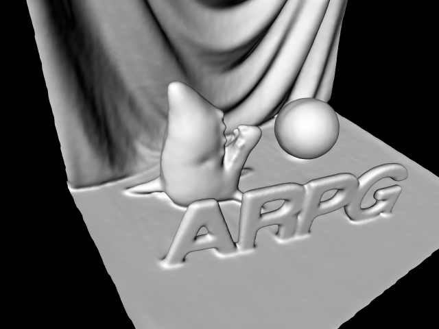
(a)

(b)

(c)

Figure 3: Input to our algorithm consists of (3(a)) 3D geometry, (3(b)) surface albedos, and (3(c)) one or more masked reference images with corresponding camera intrinsics and 6-DOF pose.

III-D Environment Light

In this work we model light using an environment map [9, 13, 19]. Instead of sampling points in 3D space, environment map lighting admits directional sampling. This representation works best when approximating lights located further from the observed scene. While many works have considered in-scene lighting examples [14, 12], we instead focus on out-of-scene sources [24, 21, 8, 2]. To compute the direct incident radiance from our environment map $L_{d}$ arriving at a point $\mathrm{p}$ we trace a ray with origin $\mathrm{p}$ in some direction $\omega$. If the ray is unobstructed by the scene geometry, point $\mathrm{p}$ will receive the full radiance traveling along $\omega$ as determined by the environment map.

To compute the radiance emitted by the environment map along a given direction, we first discretize a unit sphere into a finite number of uniformly spaced points, with each point representing a direction that can be sampled. We perform a similar discretization as described in [9] over an entire sphere. The resolution of this discretization is indicated by the number of desired rings. The spacing of points around each ring is computed to be as close to the inter-ring spacing as possible, as seen in Figure 4. When tracing a ray along a given direction we determine the nearest-neighbor direction from the discretized environment map and return its associated RGB value $\lambda$ as the emitted radiance.

IV Light Transport Equation

In this section we provide a brief overview of the light transport equation (LTE), so that the reader may better understand how we perform our light source estimation. Intuitively, the LTE describes how radiance emitted from a light source is distributed throughout a scene. Formally, we compute the exitant radiance $L_{o}$ leaving a point $\mathrm{p}$ in direction $\omega_{o}$ as:

Figure 4: Left: Top-down and Right: side view of our environment map discretization. The light depicted here consists of 21 rings and 522 total discrete directions.

$$L_{o}(\mathrm{p},\omega_{o})=\int_{\mathcal{H}^{2}}f(\mathrm{p},\omega_{o},\omega_{i})L_{i}(\mathrm{p},\omega_{i})|\cos\theta_{i}|\mathrm{d}\omega_{i}$$ (1)

This integral evaluates the amount of incident radiance $L_{i}$ arriving at $\mathrm{p}$ over the unit hemisphere $\mathcal{H}^{2}$ oriented with the surface normal found at $\mathrm{p}$. The function $f$ denotes the bidirectional reflectance distribution function (BRDF) found at point $\mathrm{p}$. The BRDF defines how much of the incident radiance arriving at $\mathrm{p}$ along $\omega_{i}$ is reflected in direction $\omega_{o}$. Finally, $\theta_{i}$ is the angle between $\omega_{i}$ and the surface normal found at $\mathrm{p}$. Figure 5 illustrates these relationships. Using Monte Carlo integration we can rewrite Eq. (1) as the finite sum:

$$L_{o}(\mathrm{p},\omega_{o})=\frac{1}{N}\sum_{i=1}^{N}\frac{f(\mathrm{p},\omega_{o},\omega_{i})L_{i}(\mathrm{p},\omega_{i})|\cos\theta_{i}|}{p(\omega_{i})}$$ (2)

where $N$ is the number of directions $\omega_{i}$ sampled from the distribution described by the probability density function (PDF) $p$. The incident radiance $L_{i}$ represents both the radiance coming directly from our light source, which we denote by $L_{d}$, and the radiance reflected off surrounding surfaces, which we denote by $L_{r}$. Given the recursive nature of path-tracing, we can effectively rewrite the incident radiance $L_{r}$ as exitant radiance $L_{o}$:

$$L_{r}(\mathrm{p},\omega)=L_{o}(\mathrm{p}^{\prime},\omega)$$ (3)

where $\mathrm{p}^{\prime}$ is the point where a ray leaving from $\mathrm{p}$ in direction $\omega$ first intersects the scene. As we recursively bounce rays around our scene the BRDF, PDF and $\cos\theta$ terms of the LTE are compounded. We refer to this product as throughput. Formally, the throughput $T$ of the $i^{\text{th}}$ point $p_{i}$ in our current path is defined as:

$$T(\mathrm{p}_{i})=\prod_{j=1}^{i}\frac{f(\mathrm{p}_{j},\omega_{j-1},\omega_{j})|\cos\theta_{j}|}{p(\omega_{j})}$$ (4)

With this definition of throughput, we can now define $L_{d}$ as:

$$L_{d}(\mathrm{p},\omega_{i})=V(\mathrm{p},\omega_{i})T(\mathrm{p})\lambda_{i}$$ (5)

where $\lambda_{i}$ is the estimated radiance for the direction in our environment map that is closest to $\omega_{i}$. The visibility function $V$ evaluates to 1 if a ray leaving from point $\mathrm{p}$ in direction $\omega_{i}$ is not obstructed by the scene geometry, and 0 otherwise.

To compute the final pixel intensity $I$, we integrate the intensities of all rays $M$ arriving at the corresponding point on our synthetic sensor (of the form of Eq. (2)). Using Monte Carlo integration we can evaluate this with the finite sum:

$$I=\frac{1}{M}\sum_{i=1}^{M}\frac{L_{o}(\mathrm{p}_{i},\omega_{i})}{p(\omega_{i})}$$ (6)

where $\mathrm{p}_{i}$ refers to the point where a ray originating from our sensor and traveling along $\omega_{i}$ first intersects with the scene. For more information on path-tracing and the LTE see [18].

\begin{overpic}[height=78.04842pt]{figures/bounce.png} \put(43.0,34.0){\large$n$} \put(43.0,3.0){\large$\mathrm{p}$} \put(22.0,23.5){\large$\omega_{o}$} \put(67.0,23.5){\large$\omega_{i}$} \put(51.0,17.5){\large$\theta_{i}$} \end{overpic}

Figure 5: Components of a single ray bounce in the LTE. $\mathrm{p}$ is the point of intersection, $\omega_{o}$ is the direction of exitant radiance $L_{o}$, $\omega_{i}$ is the direction of incident radiance $L_{i}$, $n$ is the surface normal found at $\mathrm{p}$, and $\theta_{i}$ is the angle between $n$ and $\omega_{i}$.

V Light Source Estimation

In this section we present our algorithm for light source estimation. We construct the optimization problem by first initializing all lighting parameters to be near zero, resulting in a completely dark scene. As light parameters are uniformly initialized, each light starts with the same probability of being sampled.

V-A Objective

Our objective function minimizes the photometric error between the set of original reference image $\{I_{o}\}$ and a set of corresponding reconstructed images $\{I_{r}\}$, which depict our current lighting estimation. So the photometric error $E_{p}$ can be defined as:

$$E_{p}=\sum_{i}\sum_{\mathbf{p}\in P_{i}}(I_{o,i}(\mathbf{p})-I_{r,i}(\mathbf{p}))^{2}$$ (7)

Given the prevalence of large discrepancies caused by an imperfect scene reconstruction or under-sampling, we employ the Cauchy robust norm on the raw photometric error values. Due to the potential over-parameterization of lighting, an activation penalty function is used as an additional cost. Each light direction $\lambda_{i}$ has an associated activation penalty $\Phi_{i}$ defined as:

$$\Phi_{i}=\alpha\log(1+\beta\sum_{c=1}^{n}\lambda_{i,c})$$ (8)

where $\alpha$ and $\beta$ are constant weights and $n$ is the number of channels in our images. This logarithmic cost penalizes the initial activation of a light direction but then plateaus as the intensity of light increases. Increasing the weight of $\alpha$ and $\beta$ favor solutions with fewer activated lights. The use of an activation cost has the additional benefit of completely disabling lights that can never be sampled due to the scene geometry and viewing angle of the reference images. While all lighting parameters are initialized to be near zero, if the collective probability of sampling unreachable lights is high enough, it could have a negative impact on the variance of our path-traces. This concept is explained further in the follow sections. With this additional term our final objectivation function $E$ becomes:

$$E=E_{p}+\Phi$$ (9)

V-B Light Transport Derivatives

In order to perform our light optimization we first need to compute the Jacobian of partial derivatives of pixel values with respect to the lighting parameters. We initialize the Jacobian with all values set to zero. We then populate the values of the Jacobian by tracing the given scene with our custom path-tracer. For each pixel sample we construct the path a ray of light takes as it bounces around the scene, while computing the throughput of the path as described in Section IV. When a ray eventually samples the light source, we add the ray’s final throughput to the corresponding value in the Jacobian. Following Eq. (5), we can formally define the partial derivative of the pixel $I_{i}$ with respect to the sampled light $\lambda_{j}$ for each color channel $c$ as the finite sum:

$$\frac{\partial I_{i,c}}{\partial\lambda_{j,c}}=\frac{1}{MN}\sum_{k=1}^{K}\frac{V(\mathrm{p}_{k},\omega_{j})T_{c}(\mathrm{p}_{k})}{p(\omega_{i})}$$ (10)

where $K$ is the number of samples for pixel $I_{i}$ that sample light source $\lambda_{j}$, $\mathrm{p}_{k}$ is the final point on in path $k$ before sampling the light source, and $T_{c}$ is the throughput value for color channel $c$.

In additional to the partial derivatives corresponding to the images formation, we also need to compute the partial derivatives for our activation cost. Following Eq. (8) we compute the partial derivative of the activation cost $\Phi_{i}$ with respect to the light $\lambda_{i}$ for each color channel $c$ as:

$$\frac{\partial\Phi_{i}}{\partial\lambda_{i,c}}=\frac{\alpha\beta}{1+\beta(\sum_{j=1}^{n}\lambda_{i,j})}$$ (11)

V-C Gradient Descent

Having estimated our Jacobian, we can now perform the light location and intensity optimization. As our Jacobian will typically be extremely large, dense, and exhibit no anticipated structure we can leverage, we employ gradient descent with backtracking as inverting or decomposing the Jacobian would be computationally prohibitive. To account for the inherent constraint that light parameters cannot be negative we apply gradient projection after each update [20]. We continue this process until the optimization has converged, as indicated by the Wolfe conditions on gradient magnitude [17].

V-D Sequential Monte Carlo

As described in Section V-B, we leverage importance sampling when tracing the scene, so that our estimated derivatives will exhibit a lower amount of variance while using a smaller number of samples. However, when we first construct our light optimization problem, we initialize our lighting parameters uniformly. Consequently, all lights will initially have the same probability of being sampled and we will not receive any benefit from importance sampling. If we were to formulate the optimization problem with a higher environment map resolution or use a smaller the number of samples per pixel the variance in the estimated derivatives will increase, resulting in a poorer estimate of the lighting parameters.

Yet once gradient descent converges and yields an updated set of lighting parameters we can repeat the process of estimating the derivatives. We would no longer be sampling lights uniformly, and we would now benefit greatly from importance sampling. This technique is referred to as particle filtering or sequential Monte Carlo (sMC) [15]. Our algorithm continues to re-estimate the Jacobian, retracing the scene and sampling lights according to our latest estimate of lighting parameters, and performs gradient descent until we no longer observe any significant change in the lighting parameters.

VI Experimental Results

We verified our algorithm on several distinct real and synthetic datasets. All lighting optimizations were performed using a environment map resolution of between 9 to 21 light rings and a single reference image with a resolution of $160\times 120$. We first reconstructed scene geometries for two real scenes. Albedos were manually associated with each vertices in the resulting mesh. These scene models were then used with both real and synthetic reference images.

The two experiments using real reference images were captured using Xtion Pro Live while performing scene reconstruction. These scenes were illuminated with a single white LED 1,100 lumen light bulb placed within 3 meters of the observe scene. Results for these two experiments can be seen in rows 1 and 2 of Figure 6.

We performed three additional experiments with synthetically generated reference images. There images were rendered using the same mesh and albedos used during optimization. However, there were illuminated using one or more spherical area. This was an intentional decision as not to use the same lighting model we are trying to simulate. Results for these two experiments can be seen in rows 3-5 of Figure 6. Note that the photometric error depicted in the rightmost column has been scaled up by a factor 1.5 for the sake of visualization.

All results were implemented on a GPU for derivative computation, and the optimization takes place on a CPU. Each optimization to converge took between 6-10 iterations of sequential Monte Carlo and gradient descent, which lasted for approximately 10 minutes. Once the optimization had converged, rendering the reference image took approximately 30 seconds.

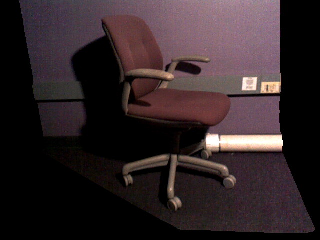
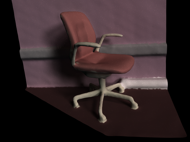
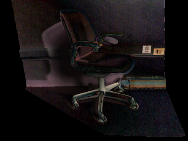
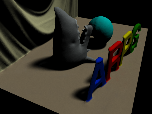
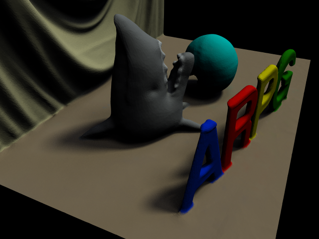
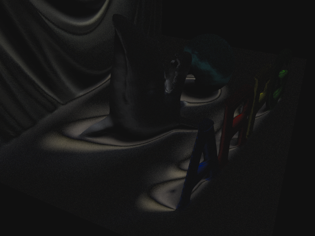
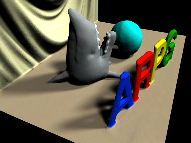
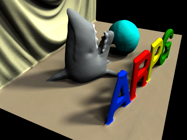
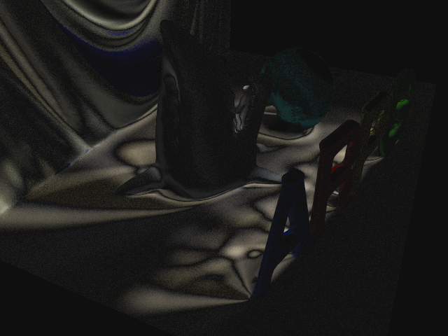
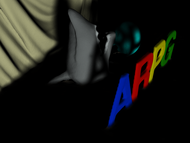
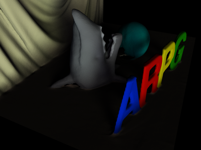
Figure 6: Left: captured reference image, Middle: render of estimated lighting conditions, Right: photometric error. Rows 1 and 2 use reference images captured with an Xtion Pro Live RGB-D camera. Rows 3-5 use reference images rendered with our path-tracer using one or two area lights.

VII Discussion

The results from our two experiments using real world reference images clearly show that the largest photometric errors often occur at depth discontinuities, due to an imperfect reconstruction of the scene’s geometry. This suggests that we may improve the robustness of our algorithm by ignoring pixels near depth discontinuities as performed [23].

We note that Figure 6 shows several departures from the generative model that are present in the image results, which can be explained through the natural behavior of our algorithm. The photometric error pane illustrates that the curtain behind the scene in the first row experiences greater photometric error as it recedes from the imaging plane. This is expected as there is no difference in the environment map’s imbuing of light in the scene dependent on in-scene depth values (the light source is modeled at infinite distance from the scene). Also, the latter three rows in Figure 6 demonstrate that the parametrization of light using an environment map do not cause a significant enough departure from an area light that would cause the scene to not appear realistic. That said, there are complicated patterns in the photometric error that result from this parametrization which do not admit a simple resolution.

Finally and most importantly, our results demonstrate that our method may be leveraged to both estimate light position and to realistically render scenes with complicated optical phenomena, including diffusing and interacting shadows and light sources. This approach is therefore a feasible option for both augmented reality applications as well as in-scene parameter estimation.

VIII Conclusion

We have presented a new algorithm for light source estimation in scenes reconstructed using a RGB-D camera. Although we model light using an environment map, we have shown that our algorithm can still accurately estimate lighting conditions created by light sources located near the observed scene. Our major contribution is developing a new technique that leverages the full expressive power of the light transport equations to perform lighting optimization. The presented optimization problem can potentially be reformulated to estimate any term of the light transport equation, namely surface albedos, bidirectional reflectance distribution functions, and scene geometry, providing a wealth of directions for future research.

References

- [1] Autonomous Robotics and Perception Group: Calibu camera calibration library (2016), http://github.com/arpg/calibu
- [2] Boom, B., Orts-Escolano, S., Ning, X., McDonagh, S., Sandilands, P., Fisher, R.B.: Point light source estimation based on scenes recorded by a RGB-D camera. In: British Machine Vision Conference, BMVC, Bristol, UK (2013)
- [3] Chen, Q., Koltun, V.: A simple model for intrinsic image decomposition with depth cues. In: International Conference on Computer Vision. pp. 241–248. IEEE (2013)
- [4] Corke, P., Paul, R., Churchill, W., Newman, P.: Dealing with shadows: Capturing intrinsic scene appearance for image-based outdoor localisation. In: Proc. of the International Conference on Intelligent Robots and Systems (IROS) (November 2013)
- [5] Duchêne, S., Riant, C., Chaurasia, G., Moreno, J.L., Laffont, P.Y., Popov, S., Bousseau, A., Drettakis, G.: Multiview intrinsic images of outdoors scenes with an application to relighting. ACM Transactions on Graphics pp. 1–16 (2015)
- [6] Goldlücke, B., Aubry, M., Kolev, K., Cremers, D.: A super-resolution framework for high-accuracy multiview reconstruction. International Journal of Computer Vision 106, 172–191 (2014)
- [7] Hachama, M., Ghanem, B., Wonka, P.: Intrinsic scene decomposition from rgb-d images. In: International Conference on Computer Vision. pp. 810–818. IEEE (2015)
- [8] Hara, K., Nishino, K., Ikeuchi, K.: Multiple light sources and reflectance property estimation based on a mixture of spherical distributions. In: 10th IEEE International Conference on Computer Vision (ICCV 2005), Beijing, China. pp. 1627–1634 (2005)
- [9] Jachnik, J., Newcombe, R.A., Davison, A.J.: Real-time surface light-field capture for augmentation of planar specular surfaces. In: International Symposium on Mixed and Augmented Reality. pp. 91–97. IEEE (2012)
- [10] Kähler, O., Prisacariu, V.A., Ren, C.Y., Sun, X., Torr, P.H.S., Murray, D.W.: Very high frame rate volumetric integration of depth images on mobile devices. IEEE Trans. Vis. Comput. Graph. pp. 1241–1250 (2015)
- [11] Kim, S.J., Pollefeys, M.: Robust radiometric calibration and vignetting correction. Transactions on Pattern Analysis and Machine Intelligence 30(4), 562–576 (2008)
- [12] Knorr, S.B., Kurz, D.: Real-time illumination estimation from faces for coherent rendering. In: Proceedings IEEE International Symposium on Mixed and Augmented Reality (ISMAR2014). pp. 113–122 (2014)
- [13] Lalonde, J.F., Matthews, I.: Lighting estimation in outdoor image collections. In: International Conference on 3D Vision. pp. 131–138. IEEE (2014)
- [14] Meilland, M., Barat, C., Comport, A.: 3d high dynamic range dense visual slam and its application to real-time object re-lighting. In: Mixed and Augmented Reality (ISMAR), 2013 IEEE International Symposium on. pp. 143–152. IEEE (2013)
- [15] Homem-de Mello, T., Bayraksan, G.: Monte carlo sampling-based methods for stochastic optimization. Surveys in Operations Research and Management Science 19, 56–85 (2014)
- [16] Mitsunaga, T., Nayar, S.K.: Radiometric self calibration. In: Computer Vision and Pattern Recognition. pp. 1374–1380 (1999)
- [17] Nocedal, J., Wright, S.: Springer-Verlag New York, 2nd edn. (2006)
- [18] Pharr, M., Humphreys, G.: Physically Based Rendering, Second Edition: From Theory To Implementation. Morgan Kaufmann Publishers Inc., San Francisco, CA, USA, 2nd edn. (2010)
- [19] Rohmer, K., Büschel, W., Dachselt, R., Grosch, T.: Interactive near-field illumination for photorealistic augmented reality on mobile devices. In: Proc. IEEE International Symposium on Mixed and Augmented Reality (ISMAR). pp. 29–38 (2014)
- [20] Rosen, J.B.: The gradient projection method for nonlinear programming. part i. linear constraints. Journal of the Society for Industrial and Applied Mathematics (1960)
- [21] Takai, T., Maki, A., Matsuyama, T.: Self shadows and cast shadows in estimating illumination distribution. In: Visual Media Production, 2007. IETCVMP. 4th European Conference on. pp. 1–10 (Nov 2007)
- [22] Whelan, T., Salas-Moreno, R.F., Glocker, B., Davison, A.J., Leutenegger, S.: Elasticfusion: Real-time dense slam and light source estimation. The International Journal of Robotics Research pp. 1–23 (2016)
- [23] Zhou, Q.Y., Koltun, V.: Color map optimization for 3d reconstruction with consumer depth cameras. ACM Trans. Graph. 33(4), 155:1–155:10 (2014)
- [24] Zhou, W., Kambhamettu, C.: Estimation of illuminant direction and intensity of multiple light sources. In: Computer Vision - ECCV 2002, 7th European Conference on Computer Vision, Copenhagen, Denmark, May 28-31, 2002, Proceedings, Part IV. pp. 206–220 (2002)