Kolmogorovian turbulence in transitional pipe flows

Abstract

As everyone knows who has opened a kitchen faucet, pipe flow is laminar at low flow velocities and turbulent at high flow velocities. At intermediate velocities there is a transition wherein plugs of laminar flow alternate along the pipe with “flashes” of a type of fluctuating, non-laminar flow which remains poorly known. We show experimentally that the fluid friction of flash flow is diagnostic of turbulence. We also show that the statistics of flash flow are in keeping with Kolmogorov’s phenomenological theory of turbulence (so that, e.g., the energy spectra of both flash flow and turbulent flow satisfy small-scale universality). We conclude that transitional pipe flows are two-phase flows in which one phase is laminar and the other, carried by flashes, is turbulent in the sense of Kolmogorov.

In 1883, Osborne Reynolds Reynolds (1883) carried out a series of experiments to test the theoretical argument, rooted in the concept of dynamical similarity, that the character of a pipe flow should be controlled by the Reynolds number $Re\equiv UD/\nu$, where $U$ is the mean velocity of the flow, $D$ is the diameter of the pipe, and $\nu$ is the kinematic viscosity of the fluid. At low $Re$, Reynolds observed a type of flow, known as laminar, in which “the elements of the fluid follow one another along lines of motion which lead in the most direct manner to their destination” Reynolds (1883). At high $Re$, Reynolds observed a type of flow, known as turbulent, in which the elements of fluid “eddy about in sinuous paths the most indirect possible” Reynolds (1883). At intermediate values of $Re$, Reynolds found a transitional regime in which the flow was spatially heterogeneous, with plugs of steady, presumably laminar flow alternating with flashes (Reynolds’s term) of fluctuating, eddying flow.

Since Reynolds’s time much has been learned about the transitional regime. It is now known that there are two types of flash Wygnanski and Champagne (1973); Wygnanski et al. (1975); Eckhardt et al. (2007); Mullin (2011); Barkley (2016): “puffs” and “slugs,” where the puffs appear first, at the onset of the transitional regime, which is triggered by finite-amplitude perturbations Mullin (2011), consistent with Reynolds’s finding that the transitional regime starts at a value of $Re$ that is highly sensitive to experimental conditions Reynolds (1883). Shaped like downstream-pointing arrowheads Wygnanski and Champagne (1973); Mullin (2011), the puffs are $\approx 20\,D$ long and travel downstream at a speed Mullin (2011) of $\approx 0.9\,U$. A puff may decay and disappear, or it may split into two or three puffs separated by intervening laminar plugs Avila et al. (2011). The tendency to decay competes with the tendency to split, which gains importance as $Re$ increases, becoming dominant Avila et al. (2011) at $Re\approx 2040$. With further increase in $Re$, the puffs are replaced by slugs Barkley et al. (2015) ($Re\gtrsim 2250$). With a head faster than $U$ and a tail that is slower, the slugs, unlike the puffs, spread as they travel downstream and are therefore capable of crowding out the laminar plugs. As $Re$ increases further, the flow turns turbulent.

Although puff flow and slug flow have been probed experimentally Wygnanski and Champagne (1973); Wygnanski et al. (1975); Mullin (2011), they have scarcely being characterized statistically, and at present it would be difficult to ascertain what the most salient differences or similarities might be between, say, the structure of puff flow and that of turbulent flow. With these considerations in mind, we start by turning our attention to $f$, a unitless measure of pressure drop per unit length of pipe. Known as “fluid friction,” $f$ is sensitive to the internal structure of a flow, and has therefore been used, ever since the time of Reynolds, to classify flows as laminar, turbulent, or transitional.

By definition, $f\equiv\frac{D\Delta P/\Delta L}{\rho U^{2}/2}$, where $\Delta P/\Delta L$ is the pressure drop per unit length of pipe and $\rho$ is the density of the fluid. For laminar flow, Reynolds Reynolds (1883) found that $f=f_{\rm{lam}}(Re)\equiv 64/Re$, in accord with a classical mathematical result, derivable from the equations of motion of a flow dominated by viscosity. Fluctuations have a marked effect on $f$, and for turbulent flow Reynolds Reynolds (1883) found that $f=f_{\rm{turb}}(Re)\equiv 0.3164Re^{-1/4}$ (see Supplementary Text in Supplemental Material (SM)). This empirical result, known as the Blasius law Schlichting (1979), provides an excellent fit to experimental data on turbulent flow for $Re<10^{5}$. The Blasius law has not yet been derived from the equations of motion, but it has recently been shown that the scaling $f_{\rm{turb}}(Re)\propto Re^{-1/4}$ can be derived from Kolmogorov’s phenomenological theory of turbulence Gioia and Bombardelli (2002); Gioia and Chakraborty (2006). Lastly, for the transitional regime, Reynolds found that the relation between $f$ and $Re$ “was either indefinite or very complex” Reynolds (1883). Our immediate aim is to take another look at this complexity.

We carry out measurements of $f$ in a 20-m long, smooth, cylindrical glass pipe of $D=2.5$ cm $\pm 10$ $\mu$m. The fluid is water. Driven by gravity, the flow remains laminar up to the highest $Re$ tested ($Re\approx 8300$). To make flashes, we perturb the flow using an iris or a pair of syringe pumps. We compute data points ($f,Re$) by measuring, at discrete times $t$, the mean velocity $U$ and the pressure drop $\Delta P$ over a lengthspan $\Delta L=202D$. The time series $\Delta P(t)$ and $U(t)$ yield $f(t)$ and $Re(t)$, which we average over a long time ($>4000$ $D/U$) to obtain a single data point $(f,Re$). (See Methods in SM for further discussion on the experimental setup.)

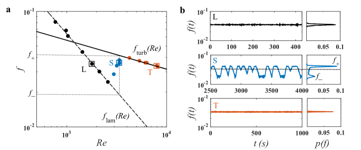
Figure 1: Experimental measurement of friction for transitional flows with slugs. These flows consist of laminar plugs and slugs. To make slugs, we perturb the flow using an iris. (a) Data points $(f,Re)$ corresponding to laminar flows (shown in black), transitional flows (shown in blue), and turbulent flows (shown in red). The dashed line is the friction for laminar flow, $f_{\rm{lam}}(Re)$; the solid line is the friction for turbulent flow, $f_{\rm{turb}}(Re)$ (the Blasius law). (b) The time series $f(t)$ and the attendant probability distribution function $p(f)$ for the data points marked L, S, and T in panel (a). Note that for the transitional data point S, $f(t)$ swings between two distinct values, $f_{-}$ and $f_{+}$, where $f_{-}=f_{\rm{lam}}(Re)$ and $f_{+}=f_{\rm{turb}}(Re)$, as indicated in panel (a). Here, $f_{-}$ is the friction for laminar plugs, confirming that laminar plugs are indeed laminar, and $f_{+}$ is the friction for slugs, suggesting that slugs are turbulent. This conclusion holds for all the transitional data points of panel (a).

In Fig. 1a, a log-log plot of $f$ vs. $Re$, we see data points that fall on $f_{\rm{lam}}(Re)$ and correspond to laminar flows; data points that fall on $f_{\rm{turb}}(Re)$ and correspond to turbulent flows; and data points that fall between $f_{\rm{lam}}(Re)$ and $f_{\rm{turb}}(Re)$ and correspond to transitional flows. Here, all transitional flows are transitional flows with slugs. In Fig. 1b, we show the time series $f(t)$ and the attendant probability distribution function $p(f)$ for a representative laminar data point (marked L), for a representative transitional data point (marked S), and for a representative turbulent data point (marked T). For point L and for point T, $p(f)$ has a single peak, the value of which is the same as the long-time average of $f(t)$, which we have denoted by $f$. By contrast, for the transitional data point S, $p(f)$ has two peaks and $f(t)$ swings Durst and Ünsal (2006) between the peak values, marked $f_{-}$ and $f_{+}$ in Fig. 1, spending little time at the long-time average of $f(t)$, which includes contributions from both laminar plugs and slugs. Here, $f_{-}$ is the friction for laminar plugs (that is, the unitless pressure drop per unit length of laminar plug) and $f_{+}$ is the friction for slugs (that is, the unitless pressure drop per unit length of slug). But there is more: it turns out that $f_{-}=f_{\rm{lam}}(Re)$ and $f_{+}=f_{\rm{turb}}(Re)$ (as indicated in Fig. 1a)—and not just for data point S but for all transitional data points in Fig. 1a. This finding confirms that laminar plugs are indeed laminar, and, more important, it suggests that slugs are turbulent.

We now turn to transitional flows with puffs. Unlike slugs, puffs are short ($\approx 20\,D$ long) as compared to the lengthspan $\Delta L=202\,D$, and the technique we have used to measure $f$ for slugs cannot be used for puffs. To measure $f$ for puffs, we create a train of puffs Samanta et al. (2011); Hof et al. (2010) such that at any given time about 6-7 puffs fit within $\Delta L$. We then measure the time series $f(t)$, which we average over a long time to obtain $f$. Now, this $f$ includes contributions from both puffs and laminar plugs. To disentangle these contributions, we use the procedure described in Methods (SM); this procedure yields $f$ for puffs and $f$ for laminar plugs. Note that the same procedure can be applied to transitional flows with slugs, as an alternative to the simpler procedure that we used to obtain the results of Fig. 1b (the results differ by $<1.5\%$).

In Fig. 2a, a log-log plot of $f$ vs. $Re$, we show all of the transitional data points that we have measured. For each of the transitional data points in Fig. 2a, we compute $f$ for flashes (either slugs or puffs, as the case might be) and $f$ for laminar plugs, and plot the results in Fig. 2b. For all transitional flows, $f$ for laminar plugs equals $f_{\rm{lam}}(Re)$ and $f$ for flashes equals $f_{\rm{turb}}(Re)$, irrespective of the type of flash. Thus, by the conventions of fluid dynamics going back to the times of Reynolds, flash flow is turbulent flow.

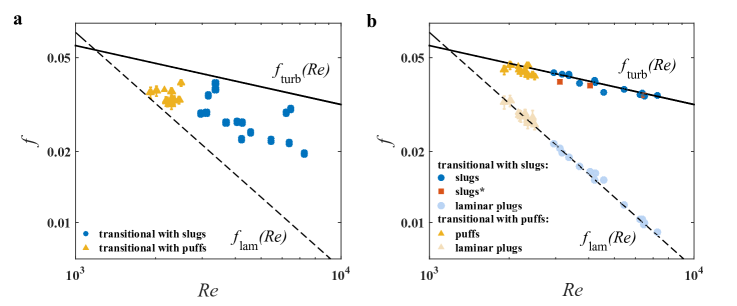
Figure 2: Experimental measurement of friction for transitional flows. (a) Data points $(f,Re)$ corresponding to transitional flows with slugs (shown in blue) and transitional flows with puffs (shown in yellow). For each data point, $f$ includes a contribution from laminar plugs and a contribution from flashes (either slugs or puffs, as the case might be). By disentangling these contributions we obtain $f$ for laminar plugs ($f_{-}$) and $f$ for flashes ($f_{+}$). In panel (b) we show the data point $(f_{-},Re)$ and the data point $(f_{+},Re)$ for each and every data point in panel (a). In all cases, $f_{-}$ falls on $f_{\rm{lam}}(Re)$, confirming that laminar plugs are indeed laminar, and $f_{+}$ falls on $f_{\rm{turb}}(Re)$, indicating that flashes, irrespective of type, are turbulent. All data points (panels a and b) have error bars. The vertical error bars indicate errors in $f$ (see Supplementary Text in SM); they are mostly smaller than the size of the data points. The errors in $Re$ are in all cases smaller than the size of the data points. In panel (b), for the data points marked with $*$, we compute $f$ for slugs using the same procedure that we use to compute $f$ for puffs.

To adduce further experimental evidence that flash flow is indeed turbulent flow, we turn to Kolmogorov’s phenomenological theory of turbulence Kolmogorov (1941); Frisch (1995), a theory that provides a thorough, empirically-tested description of the statistical structure of turbulent flow. Central to the phenomenological theory is the turbulent-energy spectrum $E(k)$, which represents the way in which the turbulent kinetic energy is distributed among turbulent fluctuations of different wavenumbers $k$ in a flow. Kolmogorov argued that, for $Re\rightarrow\infty$ and for $k$ in the “universal range” $k\gg D^{-1}$, $E(k)$ depends only on $k$, $\nu$, and $\varepsilon\propto U^{3}/D$, irrespective of the flow, where $\varepsilon$ is the turbulent power (that is, the rate at which turbulent kinetic energy is dissipated in the flow). In this case, Kolmogorov predicted that Kolmogorov (1941); Frisch (1995)

$$E(k)\propto\frac{\nu^{2}}{\eta}F(k\eta),$$ (1)

which is known as small-scale universality, and

$$\eta\propto DRe^{-3/4},$$ (2)

where $F$ is a universal function and $\eta$ is the viscous lengthscale. Further, for $k$ in the “inertial range” $D^{-1}\ll k\ll\eta^{-1}$, a subset of the universal range, $E(k)\propto\varepsilon^{2/3}k^{-5/3}$, which is known as the “5/3 law.” Eq. (1), Eq. (2), and the 5/3 law are asymptotic results associated with the limit $Re\rightarrow\infty$, and it is not possible to predict mathematically for what finite value of $Re$ they might be expected to hold within a preset tolerance. In practice, it is only feasible to verify the 5/3 law over a broad inertial range, which necessitates a small ratio $\eta/D$, which in turn necessitates a particularly large value of $Re$ (due to the small exponent of $Re$ in Eq. (2)). Indeed, in pipe flows the 5/3 law becomes clearly apparent Rosenberg et al. (2013) only for $Re>80,000$, well above the values of $Re$ at which flashes have been observed. By contrast, Eq. (1) and Eq. (2) can hold in principle at the values of $Re$ of our experiments (also see Schumacher et al. (2007, 2014)). Note, however, that whereas the 5/3 law can be tested by carrying out a single experiment at a very high value of Re, a test of Eq. (1) and Eq. (2) requires that many experiments be carried out over a broad range of values of $Re$.

To compute $E(k)$ we start by measuring a time series of the axial velocity at the centerline of the pipe, $u(t)$, using laser Doppler velocimetry (LDV). In Fig. 3a we plot $u(t)$ for three representative flows: a turbulent flow, a transitional flow with slugs, and a transitional flow with puffs; for the transitional flows, the segments of $u(t)$ corresponding to flashes have been shaded in grey. Using time series such as those of Fig. 3a, we compute $E(k)$ and $\eta$ for several turbulent flows, slug flows, and puff flows (see Methods in SM). In Fig. 3b, we show a few representative spectra $E(k)$, along with a few high-$Re$ spectra from the Princeton superpipe experiment Bailey et al. (2009); Rosenberg et al. (2013). The spectra of Fig. 3b have been rescaled in order to verify small-scale universality (Eq. (1)). At high $k\eta$, the rescaled spectra $\eta E(k)/\nu^{2}$ vs. $k\eta$ converge onto the universal function $F(k\eta)$ of Eq. (1) for turbulent flows as well as for flash flows, in keeping with small-scale universality. Further, the rescaled spectra peel off from $F(k\eta)$ at a value of $k\eta$ that lessens monotonically as $Re$ increases, irrespective of the type of flow.

In Fig. 3c, we test Eq. (2) using data points from all our experiments along with a few high-$Re$ data points from the Princeton superpipe experiment Bailey et al. (2009). Irrespective of the type of flow, the data points, which span about two decades in $Re$, are in keeping with Eq. (2). From Figs. 3b and 3c, we conclude that the spectra and the viscous lengthscales of flash flows, like those of conventional turbulent flows, are governed by the phenomenological theory of turbulence, with the implication that flash flows, aside from their being restricted to relatively low $Re$, are statistically indistinguishable from conventional turbulent flows.

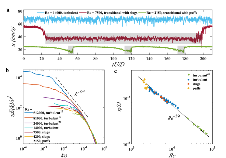
Figure 3: Tests of Kolmogorov’s phenomenological theory of turbulence, Eqs. (1) and (2), for flash flows. (a) Time series of the axial velocity $u$ at the centerline of the pipe for three representative flows. (For the transitional flow with puffs, we plot $1.5\,u(t)$ for the sake of clarity.) The segments of $u(t)$ that correspond to slugs and puffs have been shaded in grey. We use those segments to compute the spectra $E(k)$ and the viscous lengthscale $\eta$ for slug flow and for puff flow. (b) Plots of the rescaled spectra $\eta E(k)/\nu^{2}$ vs. $k\eta$ for a few representative flows, including turbulent flows and flash flows. The rescaled spectra are in good keeping with small-scale universality (Eq. (1)), irrespective of the type of flow. (c) Data points $(\eta/D,Re)$ for all our experiments and for a few high-$Re$ Princeton superpipe experiments Bailey et al. (2009), showing agreement with the Kolmogovorian scaling of Eq. (2).

In a number of experimental and computational studies Sano and Tamai (2016); Lemoult et al. (2016); Shih et al. (2016) published in 2016, compelling evidence has been adduced in support of a 30 year-old conjecture by Yves Pomeau Pomeau (1986) to the effect that the subcritical transition in pipe flow and other shear flows belongs to the directed-percolation universality class of non-equilibrium phase transitions. Yet, in a comment on those studies, titled “The Long and Winding Road,” Pomeau Pomeau (2016) cautioned that “the arrowhead patterns observed in early experiments [on boundary layers] are sufficiently regular to denote a bifurcation to a turbulence-free state.” That is to say, if flashes were non-turbulent, they could hardly be the agents of a transition to turbulence, and the experimental and computational evidence of directed percolation would be severed from the turbulent regime. Our findings indicate that, at least for pipe flow, flashes display fluid-frictional behavior diagnostic of turbulence and a statistical structure indistinguishable from that of conventional turbulent flow in the sense of Kolmogorov. Thus, we conclude that flash flow is but turbulent flow, and flashes endow the transitional regime with the requisite link to turbulence. Our findings suggest that new insights into the transition to turbulence may be gained by approaching the transition from above, from higher to lower $Re$, complementing the usual approach from below. The long road keeps winding.